Classification on manifolds

(1)

Classification on Manifolds

by Suman K. Sen

A dissertation submitted to the faculty of the University of North Carolina at Chapel Hill in partial fulfillment of the requirements for the degree of Doctor of Philosophy in the Department of Statistics and Operations Research.

Chapel Hill 2008

Approved by

Advisor: Dr. James S. Marron

Reader: Dr. Douglas G. Kelly

Reader: Dr. Mark Foskey

Reader: Dr. Martin A. Styner

(2)

(3)

ABSTRACT

SUMAN KUMAR SEN: Classification on Manifolds (Under the direction of Dr. James S. Marron)

This dissertation studies classification on smooth manifolds and the behavior of High Dimensional Low Sample Size (HDLSS) data as the dimension increases. In modern image analysis, statistical shape analysis plays an important role in under-standing several diseases. One of the ways to represent three dimensional shapes is the medial representation, the parameters of which lie on a smooth manifold, and not in the usual d-dimensional Euclidean space. Existing classification methods like Support Vector Machine (SVM) and Distance Weighted Discrimination (DWD) do not naturally handle data lying on manifolds. We present a general framework of classification for data lying on manifolds and then extend SVM and DWD as special cases. The approach adopted here is to find control points on the manifold which represent the different classes of data and then define the classifier as a function of the distances (geodesic distances on the manifold) of individual points from the con-trol points. Next, using a deterministic behavior of Euclidean HDLSS data, we show that the generalized version of SVM behaves asymptotically like the Mean Differ-ence method as the dimension increases. Lastly, we consider the manifold (S2₎d_{, and} show that under some conditions, data lying on such a manifold has a deterministic geometric structure similar to Euclidean HDLSS data, as the dimension (number of componentsdin (S2)d) increases. Then we show that the generalized version of SVM behaves like the Geodesic Mean Difference (extension of the Mean Difference method to manifold data) under the deterministic geometric structure.

(4)

ACKNOWLEDGEMENTS

I would like to express my deepest gratitude to my advisor, Professor J. S. Marron for his guidance, motivation and support. It is indeed a privilege to be his student.

I would also like to thank my committee members: Dr. Douglas G. Kelly, Dr. Mark Foskey, Dr. Martin A. Styner and Dr. Yufeng Liu for their suggestion and comments. Special thanks to Dr. Mark Foskey for making so much effort to answer my questions and providing valuable insights. He was always there to help. I thank Dr. Martin A. Styner for providing me with the data and his help to interpret the results.

I thank the MIDAG community for providing an enriching research environment, and Dr. Stephen Pizer for his extraordinary leadership. Special thanks to Dr. S. Joshi for helping me to get started with this research project. Without the gracious help of Ja-Yeon, Josh, Rohit, Ipek and Qiong, this document could not have been completed. I thank the professors and my colleagues at the Department of Statistics and Operations Research: they made my experience at UNC fruitful and enjoyable.

I express my deepest gratitude to my parents R. K. Sen and Anuradha Sen for their unconditional love, support and belief in me. I must mention my younger brother, Sumit: he is an epitome of discipline and hard work. I have learnt a few things from him.

(5)

LIST OF FIGURES

1.1 A medial atom and boundary surface of hippocampus . . . 6 1.2 The Riemannian exponential map . . . 8

2.1 Toy data on a cylinder showing the importance of geodesics . . . 16 2.2 Toy data on a sphere illustrating the effect of base point of tangency . 17 2.3 Invalid projection of m-rep illustrating the importance of working on

the manifold . . . 18

3.1 Control points on a sphere and their respective separating boundaries 22 3.2 Toy data showing the SVM hyperplane . . . 26 3.3 The m-rep sheet of a hippocampus and the surface rendering . . . 34 3.4 Performance of GMD, ITanSVM, TSVM and MSVM for Hippocampus

data . . . 35 3.5 Distance between control points against tuning parameter λ . . . 36 3.6 Change captured by GMD, ITanSVM, TSVM, MSVM for

Hippocam-pus data . . . 37 3.7 The m-rep sheet and surface rendering of a deformed ellipsoid . . . . 38 3.8 Performance of GMD, ITanSVM, TSVM and MSVM for Ellipsoid data 39 3.9 Change captured by ITanSVM, TSVM, MSVM for Ellipsoid data . . 40 3.10 Toy data showing the DWD hyperplane . . . 42 3.11 Figure showing the discontinuous nature of the MDWD objective

func-tion as a funcfunc-tion of the step size along the negative gradient direcfunc-tion. 45 3.12 Comparison of TSVM, ITanSVM, TDWD, ITanDWD for

(9)

3.13 Change captured by TSVM, ITanSVM, TDWD, ITanDWD for Hip-pocampus data . . . 47 3.14 Comparison of TSVM, ITanSVM, TDWD, ITanDWD for Ellipsoid data 48 3.15 Change captured by TSVM, ITanSVM, TDWD, ITanDWD for

Ellip-soid data . . . 49 3.16 Performance of MSVMν’s for Hippocampi data . . . 52 3.17 Performance of MSVMν’s for Ellipsoid data . . . 52 3.18 Change captured by the MSVMν directions for Hippocampus data . . 53 3.19 Change captured by the MSVMν directions for Ellipsoid data . . . . 54 3.20 Comparison of the sampling variation of MSVMν’s for Hippocampi data 54 3.21 Comparison of the sampling variation of MSVMν’s for Ellipsoid data 55

4.1 Toy data in _<2 _{illustrating the deterministic structure in Euclidean} HDLSS data . . . 62 4.2 Toy data in _<3 _{illustrating the deterministic structure in Euclidean}

HDLSS data . . . 65

(10)

CHAPTER 1

Introduction

1.1 Motivation

Statistical shape analysis is important in but not limited to understanding and diagnosing a number of challenging diseases. For example, brain disorders like autism and schizophrenia are often accompanied by structural changes. By detecting the shape changes, statistical shape analysis can help in diagnosing these diseases. One of the many ways to represent anatomical shape models is a medial representation or M-rep. The medial locus, which is a means of representing the “middle” of a geometric object, was first introduced by Blum (1967). Its treatment for 3D objects is given by Nackman and Pizer (1985). The medial atom represents a sampled place in the medial locus. Atoms form the building blocks for m-reps. In particular, the m-rep sheet can be thought of as representing a continuous branch of medial atoms. For details of discrete and continuous m-reps, see Pizeret al. (1999) and Yushkevich

et al. (2003) respectively. The M-rep approach has proven to be useful in describing various aspects of shape, in capturing important summaries of the object’s interior and boundary, and in providing relationships between neighboring objects. A major advantage of the m-reps approach to object representation over competitors is that it allows superior correspondence of features across a population of objects, which is critical to statistical analysis.

(11)

manifold, and not in the usual Euclidean space. We are interested in classification of data which lie on this curved m-rep space. A major contribution of this work is to use the geometric information inherent to the manifold. This enables the capture of a wide range of nonlinear shape variability including local thickness, twisting and widening of the objects. Principal geodesic analysis, the nonlinear analog of principal component analysis in this type of manifold setting, was developed using the geom-etry that can be derived from the Riemannian metric, including geodesic curves and distances (see Fletcher et al., 2003, 2004) . Classification methods like Fisher Lin-ear Discrimination (Fisher, 1936), Support Vector Machines (see Vapniket al., 1996; Burges, 1998), Distance Weighted Discrimination (Marronet al., 2004) were designed for data which are vectors in Euclidean space and do not deal extensively with data that are parameterized by elements in curved manifolds. See Duda et al. (2001) and Hastie et al. (2001) for an overview of common existing classification methods. The challenge addressed here is to develop classification methods, or extend the existing methods so that they can handle data in curved manifolds. The notion of separating hyperplane, fundamental to many Euclidean classifiers, is challenging to even define in manifolds. The approach adopted here is to find control points on the manifold which represent the different classes of data and then define the classifier as a function of the distances (geodesic distances on the manifold) of individual points from the control points. We thus bypass the problem of explicitly finding separating bound-aries on the manifold. The control points chosen will be those which optimize some objective function and the performance of several reasonable objective functions will be investigated and compared.

This approach will enable us not only to use the method on our motivating example of m-rep data (Senet al., 2008), but it is also applicable for Diffusion Tensor Magnetic Resonance Imaging (DT-MRI), and several other sciences like human movement, mechanical engineering, robotics, computer vision and molecular biology where

(12)

Euclidean data often appear.

Data sets with more variables (i.e., attributes or entries in the data vector) than observations are now important in many fields. This type of data is called High Dimension Low Sample Size (HDLSS) data. For example, in genetics a typical mi-croarray gene expression data set has the number of genes ranging from thousands to tens of thousands, while the number of tissue samples (i.e., observations) is typically less than several hundreds. Data from medical imaging, and from text recognition also often have a much larger dimension dthan the sample size n. In our motivating example of m-reps, we have the HDLSS situation too, but the entries in each dimen-sion are not Euclidean. As pointed out earlier, they lie on a smooth manifold. Due to the limitations of human visual perception beyond three dimensions, the behav-ior of HDLSS data is often counter-intuitive (Hall et al., 2005; Donoho and Tanner, 2005), even in the Euclidean case. Ge and Simpson (1998) provided a framework for evaluating dimensional asymptotic properties of classification methods such as the Mean Difference. For the Euclidean case, Hall et al. (2005) have studied some deterministic behavior of the data and used the observations to analyze the asymp-totic properties (asd_{→ ∞}) of classification methods such as Mean Difference, SVM, DWD and One-Nearest-Neighbor. As a part of this dissertation, we have studied some geometric properties of HDLSS manifold data and used them to analyze the asymptotic behavior of one of our proposed methods, which is an extension of SVM for manifold data.

1.2 Overview of Chapters

This dissertation has been organized into chapters as follows:

Section 1.3 gives an overview of the medial representation. Section 1.4 gives an overview of different statistical methods for manifold data and m-reps.

(13)

contains a literature review of popular classification methods like Mean Difference, Fisher Linear Discrimination, Support Vector Machines, Distance Weighted Discrim-ination. Section 2.3 illustrates why these methods are not always ideal for data on manifolds.

Chapter 3 presents the key ideas of our methods. Section 3.1 introduces the fundamental idea of control points, and based on it proposes the general classification rule. Section 3.1.2 illustrates the importance of a reasonable choice of control points. Section 3.3 gives a brief overview of SVM, and generalizes it to manifold data. It also provides a solving algorithm to the resulting optimization problem. Section 3.4 gives a brief overview of DWD, and develops an optimization problem which generalizes DWD to work with manifold data.

Chapter 4 studies some geometric properties of HDLSS data. Section 4.1 briefly discusses some deterministic properties of Euclidean HDLSS data and studies the asymptotic behavior (as dimension d _{→ ∞}) of one of our developed methods (mani-fold SVM, also called MSVM) under such conditions. Section 4.2 studies conditions under which there is a deterministic structure in HDLSS manifold data. This deter-ministic structure is then used to study some properties of the MSVM method.

Chapter 5 discusses some avenues for future research, involving unresolved ques-tions and possible applicaques-tions of the developed methods in new areas.

The next section gives an overview of the medial locus and some of its mathemat-ical properties. It describes m-reps and the deformable models approach based on them. The deformable m-reps approach to image segmentation is described by Pizer

et al. (2003). A fine overview of medial techniques that goes beyond the material covered in this section can be found in the Ph.D. dissertation of Yushkevich (2003) and the book by Siddiqi and Pizer (2007).

(14)

1.3 The Medial Locus and M-reps

The medial locus is a means of representing the “middle” or “skeleton” of a geo-metric object. Such representations have found wide use in computer vision, image analysis, graphics, and computer aided design (Bloomenthal and Shoemake (1991); Storti et al. (1997)). Psychophysical and neurophysiological studies have shown ev-idence that medial relationships play an important role in the human visual system (Leyton (1992); Lee et al. (1995)). The medial locus was first proposed by Blum (1967), and its properties were later studied in 2D by Blum and Nagel (1978) and in 3D by Nackman and Pizer (1985). The definition of the medial locus of a setA_{∈ <}n is based on the concept of a maximal inscribed ball.

(15)

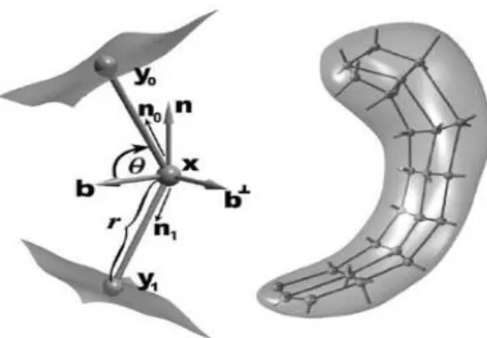
Figure 1.1: Medial atom with a cross section of the boundary surface it implies (left). An m-rep model of a hippocampus and its boundary surface (right).

The medial manifold is sampled over an approximately regular lattice and the elements of this lattice are called medial atoms. A medial atom (Fig. 1.1) is defined as a 4-tuple m = _{x, r, n0, n1}, consisting of: x ∈ <3, the center of the inscribed sphere; r _{∈ <}+_{, the local width defined as the common spoke length;} _n

o, n1 ∈ S2 , the two unit spoke directions (represented as points onS2, the unit sphere in_<3). The medial atom implies two opposing boundary points, yo, y1, called implied boundary points, which are given by

y0 =x+rn0 and y1 =x+rn1. (1.1)

The surface normals at the implied boundary pointsy0, y1 are given byn0, n1, respec-tively.

A medial atom, as defined above, is represented as a point on the manifold _M(1) =

<3 _{× <}+ _×_S2 _×_S2_. _{Moreover, an m-rep model consisting of} _n _{medial atoms may} be considered as a point on the manifold cartesian product _M(n) = Qn_i=1_M(1). This space is a particular type of manifold known as a Riemannian symmetric space, which simplifies certain geometric computations, such as computing geodesic dis-tances. We briefly review some of the concepts now. See Boothby (1986); Helgason (1978); Fletcher (2004), Fletcher et al. (2003, 2004) for more details. Pizer et al.

(16)

(1999) describes discrete m-reps. For details on continuous m-reps, see Yushkevich

et al. (2003); Terriberry and Gerig (2006).

1.3.1 Riemannian metric, Geodesic curve, Exponential and

Log maps

ARiemannian metricon a manifoldM is a smoothly varying inner product<_·,_·>

on the tangent plane TpM at each point p ∈ M. The norm of a vector X ∈ TpM is given by _||X_|| =< X, X >(1/2)_{. The Riemannian distance between two points}

x, y _∈ M, denoted by d(x, y), is defined as the minimum length over all possible smooth curves between x and y. A geodesic curve is a curve that locally minimizes the distance between points.

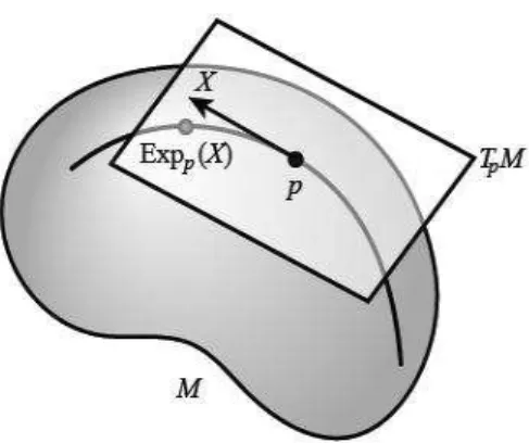
Given a tangent vector X _∈ TpM, there exists an unique geodesic, γX(t), with

X as its initial velocity. The Riemannian exponential map, denoted by Expp, maps

X to the point at time one along the geodesic γX. The exponential map preserves distances from the initial point, i.e., d(p,Exp_p(X)) = _||X_||. In the neighborhood of zero, its inverse is defined and is called the Riemannian log map, denoted by Log_p. Thus, for a point y in the domain of Log_p, the geodesic distance between p and y is given by

d(p, y) = _||Logp(y)|| (1.2)

1.3.1.1 Exponential and Log maps for S2

On the sphere S2_{, the geodesics at the base point} _p _{= (0}_,₀_,_{1) are great circles} through p. If we consider the tangent vectorv = (v1, v1,0)∈TpS2 in the x−yplane, the exponential map at pis given by

Expp(v) = (v1.

sin_||v_||

||v_|| , v2.

sin_||v_||

(17)

Figure 1.2: The Riemannian exponential map at p_∈M. X _∈TpM

where _||v_||=pv2 1 +v22.

The corresponding log map for a point x= (x1, x2, x3)∈S2 is given by

Logp(x) = (x1.

θ

sinθ, x2. θ

sinθ) (1.4)

where θ = arccos(x3) is the spherical distance from the base point p to the point x. Note that the antipodal point ₋pis not in the domain of the log map.

1.3.1.2 Exponential and Log maps for M-reps

Recall, from first part of Section 1.3 that the medial atom m = _{x, r, n0, n1} ∈

M(1) =_<3_{× <}+_×_S2_×_S2 _{and a m-rep model consisting of} _n _{medial atoms may be} considered as a point on the manifold _M(n) = Qn_i=1_M(1). Let p = (0,1, p0, p1) ∈

M(1) be the base medial atom, where p0 = p1 = (0,0,1) are base points for the spherical components. Let us write a tangent vectoru_∈TpM(1) as u= (x, ρ, v0, v1), where x _{∈ <}3 _{is the positional tangent component,} _ρ _{∈ <} _{is the radius tangent} component, and v0, v1 ∈ <2 are the spherical tangent component. Then, for M(1) we have

Expp(u) = (x, eρ,Expp0(v0),Expp1(v1)) (1.5)

(18)

where the Exp maps on the right-hand side are the spherical exponential maps given by equation (1.3). Likewise, the log map of m=_{x, r, n0, n1} is

Log_p(m) = (x,logr,Log_p0(n0),Log_p1(n1)) (1.6)

where the Log maps on the right-hand side are the spherical log maps given by (1.4). Finally, the exponential and log maps for the m-rep model space _M(n) is the cartesian product of corresponding maps in _M(1).

The norm for vector u_∈TpM(1) is

||u_||= (_||x_||2+ ¯r2(ρ2+_||v1||2+||v2||2)) 1

2 (1.7)

and the geodesic distance between two atoms m1, m2 ∈ M(1) is given by

d(m1, m2) = ||Logm1(m2)||=||Logm2(m1)|| (1.8)

1.4 Statistical Methods on M-reps and on General

Manifolds

(19)

dis-tributions on Lie groups. Pennec (1999) defines Gaussian disdis-tributions on a manifold as probability densities that minimize information. Bhattacharya and Patrangenaru (2002) develop nonparametric statistics of the mean and dispersion values for data on a manifold. Mardia (1999) describes several methods for the statistical analysis of directional data, i.e., data on spheres and projective spaces. Kendall (1984) and also Mardia and Dryden (1989) have studied the probability distributions induced on shape space by independent identically distributed Gaussian distributions on the landmarks. Similar ideas in the theory of shape were independently developed by Bookstein (1978, 1986). Ruymgaart (1989) studied convergence of density estimators on spheres. Ruymgaartet al.(1992) gave a Rao-Cramer type inequality on Euclidean manifolds. Olsen (2003) and Swann and Olsen (2003) describe Lie group actions on shape space that result in nonlinear variations of shape. Klassen et al. (2004) de-velop an infinite-dimensional shape space representing smooth curves in the plane. Chikuse (2003) concentrates on the statistical analysis of two special manifolds, the Stiefel manifold and the Grassmann manifold, treated as statistical sample spaces consisting of matrices.

A standard technique for describing the variability of linear shape data is principal component analysis (PCA), a method whose origins go back to Pearson (1901) and Hotelling (1933). One of the earliest applications of PCA in functional data analysis was given by Rao (1958). Its use in shape analysis and deformable models was introduced by Cooteset al.(1993). Principal geodesic analysis, the nonlinear analog of principal component analysis in this type of manifold setting was developed using the geometry that can be derived from the Riemannian metric, including geodesic curves and distances (see Fletcheret al.(2003, 2004)). A popular approach to handling data in manifolds is “Kernel Embedding” (see Sch¨olkopf and Smola (2002)) where the data are mapped to a higher dimensional feature space.

The next chapter provides a brief overview of the problem of classification. It also

(20)

(21)

CHAPTER 2

Overview of Classification

The first section gives the general setup followed by a description of popular methods in Section 2.2. The last section explains why these methods fail in the context of data naturally understood to be lying on curved manifolds. See Dudaet al. (2001) and Hastie et al. (2001) for an overview of common existing classification methods. Note that, in the literature, classification and discrimination are interchangeable terms. In our discussion we mostly refer to it as classification.

2.1 The Problem of Classification

Let Xi denote the attributes that describe the ith individual and Yi denote its group label, i = 1,2, . . . , n. Xi can be vector valued (in most cases it is a high dimensional vector) whileYi is a scalar taking values in the set{1,2, . . . , K} if there are K classes. In our discussion, we will always have only two classes. For some mathematical convenience, let the corresponding labels Y _{∈ {−}1,1_}.

Given a set of individuals (and their group labels), the goal of classification meth-ods is to find a rule f(x) that assigns a new individual to a group on the basis of its attributes X.

2.2 Popular Methods of Classification

(22)

to it. It is the optimal classification rule when the data comes from distributions which only differ by their means and have common covariance matrix, which is the identity. A classical approach to improve the Mean Difference method was proposed by Fisher (1936), now called Fisher Linear Discrimination (FLD). It is the optimum rule when the two classes is assumed to have the same covariance matrix (but not limited to the identity). Since FLD approaches the problem by sphering the data it is frequently useless in many modern day applications, particularly High Dimension Low Sample Size (HDLSS) situations, where we cannot calculate the inverse of the covariance matrix.

The Support Vector Machine (SVM), proposed by Vapnik (1982, 1995) is a pow-erful classification method used in HDLSS situations. See Burges (1998) for a lucid overview. Marron et al. (2004) showed that SVM suffers from “data piling” at the “margin” and introduced a related method called Distance Weighted Discrimina-tion (DWD). DWD avoids data piling and improves generalizability of the decision rule. Both SVM and DWD are “linear” classifiers in the sense that the rules are linear functions of the data vector. Geometrically, the separating surface they pro-vide is a linear hyperplane and thus cannot separate data which need a nonlinear separating boundary. This problem is overcome by “kernel embedding”. The data vectors are embedded in a higher dimensional space where linear methods, such as SVM can be much more effective. The book by Sch¨olkopf and Smola (2002) gives a fine overview of the kernel methods. Readers can also visit http://www.kernel-machines.org/publications.html for a list of publications on kernel methods.

(23)

2.3 Value Added by Working on Manifolds

Recall that our goal is to help image analysts and doctors understand how two groups of objects differ. For example, let us consider a study of shapes of hippocampi for groups of schizophrenic and normal individuals. There is a strong interest in knowing whether the occurrence of the disease is actually accompanied by a struc-tural difference of the hippocampus. If there is an association, the next question is how these shapes change as we look at the direction of separation.

Some common approaches to handling data on manifolds are:

• Flatten, as for data on a cylinder (Section 2.3.1).

• Work in the tangent plane, with base as the overall geodesic mean of the data (Section 2.3.2).

• Treat data as points embedded in a higher dimensional Euclidean space (Section 2.3.3).

The drawbacks of these approaches are illustrated in the above mentioned subsec-tions.

2.3.1 Importance of Geodesic Distance on Manifolds

Throughout our discussion, the geodesic distance will play a crucial role. Let us use an example to explain its importance.

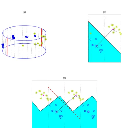
Fig. 2.1(a) shows a cylinder with data points on its surface (different symbols denote different classes). Fig. 2.1(b) shows the same data set when the cylinder is flattened. The Mean Difference decision rule (given by the two shaded regions: blue and white) is calculated by using the usual Euclidean distance on the flattened two dimensional plane. This approach is not ideal. For example, it ignores the fact that

(24)

(25)

(a)

C₁

C₋₁ (b)

C₁

C₋₁ (c)

Figure 2.1: (a): Toy data on the surface of a cylinder. Different colors (with symbols) denote different groups. (b): Data on the flattened cylinder. Shaded regions show the Mean Difference rule using Euclidean distance. A point (green star) is misclassified. (c): Tiled flattened planes capturing the structure (periodicity) of the manifold. Geodesic distance used to construct the Mean Difference rule which has no misclassified points. The red dotted line is the Mean Difference separating surface if Euclidean distance is used. c1 and c−1 are means of the classes in each case.

(26)

2.3.2 Choice of base point for Euclidean Classification on the

Tangent Plane

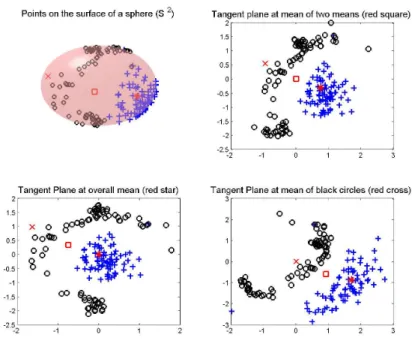
As pointed out in the Sections 1.1 and 1.4, when data appear in a small neigh-borhood, some statistical analysis, such as finding means and Principal Component Analysis can be successfully implemented. This is done in the tangent plane by projecting the data from the manifold to the tangent plane with base point as the geodesic mean (see Fletcher et al., 2003, 2004). This suggests implementing SVM and DWD in the tangent plane at the geodesic mean of the data. Fig 2.2 shows why this might not always be a good idea. In particular, this example shows that we can end up with a tangent plane where the data is not linearly separable while there is another tangent plane where separation is possible. Thus, the choice of the base point is a crucial issue.

(27)

2.3.3 Validity and Interpretability of Projections

Another approach to handle manifold data is standard Euclidean SVM and DWD, treating the data as points embedded in the higher dimensional Euclidean space. For example, planar angles (θ _∈ (₋π, π)) can be considered as embedded in _<2 _(as (sin(θ),cos(θ))), while naturally they are understood to be lying on a one-dimensional manifold (the unit circle in _<2_{). Similarly solid angles are embedded points in} _<3 while naturally they are points restricted to the surface of the unit sphere (S2_{) in}

<3_{. A separating rule will be obtained by taking this approach, but geometrically the} separating surface will not relate properly to the manifold. For example, in case of data on the surface of a sphere a separating plane cutting through the sphere will be obtained. This will probably not give a geodesic (in this case, a great circle), which is the analog of a separating hyperplane.

More importantly, when the original data is projected on to the separating direc-tion, most of them will be somewhere inside the sphere and not the surface. These projections are not interpretable because they are not valid representations of shape objects. Recall, in this example, our data objects must lie on the surface of the sphere.

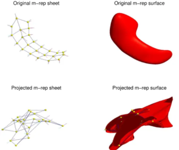
Original m−rep sheet Original m−rep surface

Projected m−rep sheet Projected m−rep surface

Figure 2.3: Top left and right: Original m-rep sheet of a hippocampus and its surface rendering respectively. Bottom left: M-rep model projected on to the separating direction (obtained when data objects are considered as points in_<240). Since it is not in the manifold it is not a valid m-rep. Bottom right: Surface rendering of the m-rep sheet on the left. It is not an interpretable shape object.

(28)

To emphasise this issue consider Figure 2.3. The upper figure is the medial repre-sentation of a human hippocampus. In our study we had two groups: 56 patients and 26 controls (see Styner et al. (2004)). Each of these models have 24 medial atoms, placed in a 8_×3 lattice (see Fig. 2.3, top left). Therefore, each of these figures belong to_M(24) =_{<3_{× <}+_×_S2_×_S2_}24_{. But when standard SVM is implemented on the} data we consider them as elements of_{<3_{× < × <}3_{× <}3_}24 ₌_<240_{. Naturally, when} we project the data sets on to the separating directions, what we get back are also elements of _<240 and not in _M(24). Therefore the projection is not a valid medial representation and thus not interpretable (Fig. 2.3, bottom panels). This motivates our approach to work on manifolds.

(29)

CHAPTER 3

Classification on Manifolds

The main problem with classification on manifolds is that it is very difficult to derive analytical expressions for geodesics and separating surfaces. Recall, from Sec-tion 1.3, a geodesic is the local shortest path along the manifold and the distance between two points is obtained as the arc length of this geodesic. Our goal is to ex-tend the idea of a separating hyperplane (which is the foundation of many Euclidean classification methods such as Mean Difference, FLD, SVM and DWD) to data lying on a manifold. A major challenge is to find an appropriate manifold analog of the separating hyperplane. Our solution is based on the idea of control points (and the geodesic distance of data from these control points), as described in the following section.

3.1 Control Points and the General Classification

Rule

We think about control points as being representatives of the two classes. If we name the control points asc1andc−1, then we propose the classification rulefc1,c−1(x) given by

fc1,c−1(x) = d 2₍_c

(30)

where c1, c−1, and x ∈ M and d(·,·) is the geodesic distance metric defined on the manifoldM. This rule assigns a new pointxto class 1 if it is closer toc1 thanc−1, and to class -1 otherwise. It is important to note here that the formulation also provides us with an implicitly defined separating surface and a direction of separation.

3.1.1 The Implied Separating Surface and Direction of

Sep-aration

The zero level set of fc1,c2(·) is the analog of the separating hyperplane, while the geodesic joining c1 and c−1 is the analog of the direction of separation. Thus, the separating surface is the set of points which is equidistant from c1 and c−1. If we denote it byH(c1, c−1), we can write,

H(c1, c−1) = {x∈M :fc1,c−1(x) = 0}

= _{x_∈M :d2(c1, x) = d2(c−1, x)} (3.2)

In d-dimensional Euclidean space, H(c1, c−1) is a hyperplane of dimension d−1 that is the perpendicular bisector of the line segment joining c1 and c−1 (see Lemma 3.1.1). Note that the Mean Difference method is a particular case of this rule, where the control points are the means of the respective classes. Similarly, the general control point classifier reduces to Fisher Linear Discrimination in Euclidean space by taking the control points as the means of the sphered data (using the pooled within class covariance estimate).

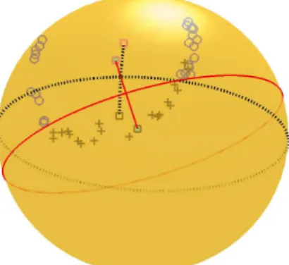
On the sphere (S2_),_H₍_c

1, c−1) is the great circle equidistant fromc1 andc−1 (see Fig. 3.1.) This shows that this approach provides us with an useful representation of a separating surface, that avoids the need to explicitly solve for it, which can be intractable as pointed out earlier.

(31)

Figure 3.1: Two pairs of control points showing their respective separating boundary and separating direction on the surface of the sphere. Different colors (with symbols) represent classes. The solid red surface (great circle) separates the data better than the dotted black surface.

are classified correctly byH(c1, c−1). Mathematically, the training set T is said to be separable byH(c1, c−1), if, ∀xi ∈T, i= 1,2, . . . , n,

fc1,c−1(xi)

    

>0 if yi = 1

<0 if yi =−1

(3.3)

Lemma 3.1.1. Consider the separating surface defined in equation (3.2). Let the data live in _<d_{. Then}

(1) H(c1, c−1) is a d−1 dimensional hyperplane.

(2) The level set of fc1,c−1(x) =k is a hyperplane, parallel to H(c1, c−1).

(3) The distance of any point x from the separating surface H(c1, c−1) is given by

d(x, H(c1, c−1)) = |

fc1,c−1(x)| 2d(c1, c−1)

(3.4)

Proof. Since the space in which the data live is Euclidean, the distance between any

(32)

two points x, y _{∈ <}d _{is given by}

d(x, y) = _||x₋y_||

= p(x₋y)T₍_x₋_y₎_. _(3.5)

Therefore, we can write the following:

fc1,c−1(x) = d 2₍_c

−1, x)−d2(c1, x)

= (c₋1−x)T(c−1−x)−(c1−x)T(c1 −x)

= wTx+b, (3.6)

wherew= 2(c1−c−1) andb = (cT−1c−1−cT1c1). Thus, the equation of the level set of

fc1,c−1(x) =k, for any k can be written as

wTx+b=k

⇒wT_x_{+ (}_b₋_k_{) = 0} _(3.7)

Note, that Equation (3.7) says that for all k, the level set is a d₋1 dimensional hyperplane with common normal vector w and intercept b₋k. This proves part (i), as we note that H(c1, c−1) is the level set for k = 0. Moreover, for any other k 6= 0, the normal to the resulting hyperplane is the same (=w). This proves part (ii).

For part (iii), we use the fact that the distance from any point z to a plane

wT_x₊_b_{= 0 is given by} |wTz+b|

||w_|| . Therefore, using equation (3.6) we can write the

distance of any point x fromH(c1, c−1) as

d(x, H(c1, c−1)) = |

wT_x₊_b_|

(33)

= |fc1,c−1(x)|

||2(c1−c−1)||

,

=

fc1,c−1(x) 2d(c1, c−1)

(3.8)

3.1.2 Choice of Control Points

Having set the framework for the general decision rule for manifolds the critical issue now is the choice of control points. For example, Fig. 3.1 shows that for the given set of data, the control points corresponding to the red solid separating boundary do a better job of classification than the pair corresponding to the black dotted boundary. So, the key to the construction of a good classification rule is to find the right pair of control points.

The rest of the chapter develops new methods for finding control points. The first approach, motivated by Mean Difference, chooses the control points as the geodesic means and is called the Geodesic Mean Difference (GMD) Method. Then we propose methods to extend SVM and DWD for manifold data.

3.2 The Geodesic Mean Difference (GMD) Method

This is motivated by the Mean Difference method in the Euclidean case. Here we replace the Euclidean means of the two classes by their geodesic means. This is a special case of the general classification rule (3.1) when c1 and c−1 are the geodesic means of the two groups of data. The geodesic mean m of a set of observations

x1, x2, . . . , xn ∈M is defined as

m= argmin p∈M

n

X

i=1

d2(p, xi). (3.9)

(34)

See Fletcher et al. (2003, 2004) and Pennec (1999) for more details. In Fig. 3.1, the black dotted great circle shows the GMD separating surface. The two square points (joined by dotted black curve) are the geodesic means of the two classes. Some points have been misclassified by this rule.

3.3 Support Vector Machine on Manifolds

This section generalizes SVM to the manifold case. Two new approaches have been developed here. In the following subsection, we review the standard SVM method.

3.3.1 A Brief Overview of Support Vector Machine (SVM)

SVM is a recently developed method which has been successfully implemented in a wide variety of applications involving classification. Here, we review this method in a simple set up. Let us first assume that the training data set is linearly separable, i.e., there is a linear classifier that can have zero training error. Consider a linear classifier f(x) =wT_x₊_b_{. The SVM first finds two hyperplane margins (over} _w _and

b) which are defined by f(x) = _±1, such that there are some observations on the margins and there are no observations between these two margins. The points on the margin are called “support vectors”. The SVM finds w and b such that the distance between the margins (which is equal to 2

||w||) is maximized. The hyperplane between the two margins: f(x) = 0 is the SVM discrimination hyperplane. Given w and b, the class label +1 is given to a new sample xi, if f(xi)>0 and the class label ₋1 is given if f(xi)<0. The SVM optimization problem overw and b is given by:

minimizew,b ||w|| 2 2

subject toyif(xi)≥1; i= 1, . . . , n, (3.10)

(35)

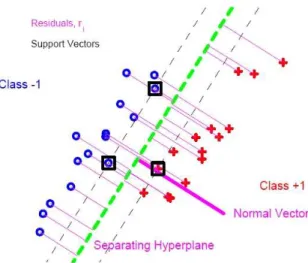
Figure 3.2: SVM hyperplane (broken green line) to separate two classes, represented by crosses and pluses. The purple vector is the SVM direction of separation.

yif(xi)≥1, i= 1, . . . , n indicate that the f(x) must classify all the samples in the training data set correctly. The distance of a pointxi from the separating hyperplane is denoted asri.

Figure 3.2 shows the SVM separating hyperplane (green dashed line) for classi-fying a toy data set, with the two classes represented by blue circles and red pluses respectively. The support vectors are shown in black boxes. The distanceri’s of only these support vectors play a role in determining the separating hyperplane.

The next subsection extends SVM to manifold data by iteratively constructing tangent planes on the manifold and implementing Euclidean SVM on the tangent planes. We call this method Iterative Tangent Plane SVM (ITanSVM).

3.3.2 Iterative Tangent Plane SVM (ITanSVM)

In this section, we propose an extension of SVM in Euclidean space to manifold data. A common approach is to implement SVM in the tangent plane at the overall mean of the data. In Section 2.3.2, we have discussed possible drawbacks of this approach which arises out of taking the point of tangency at a predetermined point (the geodesic mean). Thus, when classification is done on the tangent plane, the choice of the base point is a crucial issue. This motivates the need to find the base

(36)

point that is determined by the separability of the data in the tangent plane. In particular, we develop an iterative approach with changing point of tangency.

We start with the overall geodesic mean as the initial base point and implement Euclidean SVM in that tangent plane. Given the SVM separating hyperplane, we find out the pair of points (on the tangent plane) which determine that hyperplane and is closest to the present pair of control points (the geodesic means of the two classes, mapped to the tangent plane). The next point of tangency is taken to be the geodesic mean of the new pair of control points (after being mapped back to the manifold). We repeat these steps until convergence. The detailed algorithm is given below:

1. Let c0

1 = mean of the data in class 1 and c0−1=mean of the data in class 2. Let

b0 = mean(c01, c0−1). The superscript of zero means it is the present solution.

2. Compute the tangent plane Tb0M at b0 and find the separating hyperplane

w0_x₊_b_{= 0 by doing linear SVM on} _T b0M. 3. Given (w, b), find Lc1

1, Lc1−1 ∈ Tb0M that minimize the sum of the squares of their respective distances to Log_b0(c0

1) and Logb0(c0−1), subject to the constraint that w0_x₊_b _{is the perpendicular bisector of the the line segment joining} _Lc1 1

and Lc1 −1. 4. If_{d2_(Log

b0(c01), Lc1) +d2(Logb0(c0₋1), Lc−1)}is very small then stop. Otherwise go to the next step.

5. Set c0

1 = Expb0(Lc11) and c0−1 = Expb0(Lc1−1) and then compute b0 = mean(c01,

c0

−1). Go to step 2.

(37)

points after the first iteration. In this example, ITanSVM solution does a better job of classification than GMD (given by the dotted black great circle).

3.3.3 The Manifold SVM (MSVM) method

An unappealing feature of ITanSVM is the continual approximation of the data by projections on to the tangent plane. MSVM appears to be the first approach where all calculations are done on the manifold. MSVM determines a pair of control points that maximizes the minimum distance to the separating boundary. While the SVM criterion has many interpretations, it is the maximum margin idea that generalizes most naturally to manifolds where some Euclidean notions such as distance, are much more readily available than other (e.g., inner product). The mathematical formulation of the method and an algorithm for solving the resulting optimization problem are given below.

As given in equation (3.1), the decision function fc1,c−1(x) is

fc1,c−1(x) = d 2₍_c

−1, x)−d2(c1, x)

The zero level set of fc1,c−1(·) defines the separating boundary H(c1, c−1) for a given pair (c1, c−1). Also, let Xb(c1,c−1) denote the set (to handle possible ties) of

training points which are nearest to H(c1, c−1). We would like to solve for some ˜c1 and ˜c₋1 such that

( ˜c1,˜c−1) = argmax c1,c−1∈M

min

i=1...nd(xi, H(c1, c−1)) (3.11) In other words, we want to maximize the minimum distance of the training points from the separating boundary. Recall, from Chapter 2, that as in the classical SVM literature, we denote yi to be the class label taking values -1 and 1.

By Lemma 3.1.1, in Euclidean space, note that the distance of any point x from

(38)

the separating boundary H(c1, c−1) is

d(x, H(c1, c−1)) =

fc1,c−1(x) 2d(c1, c−1)

(3.12)

Therefore, for a separable training set (see Section 3.1), using (3.3) and (3.12), we can write the distance from the training points to the separating surface as

d(x, H(c1, c−1)) =

yfc1,c−1(x) 2d(c1, c−1)

, (3.13)

wherey=_±1 is the class label forx. Relation (3.13) will be used as an approximation that is reasonable for data on manifolds lying in a small (convex) neighborhood as this is directly computable for manifold data. Then, using (3.13) in (3.11) we would like to solve for some ˜c1 and ˜c−1 such that

( ˜c1,˜c−1) = argmax c1,c−1∈M

min i=1...n

yifc1,c−1(xi) 2d(c1, c−1)

(3.14)

It is important to note that the solution of ( ˜c1,c˜−1) in (3.14) is not unique. In fact, in the d-dimensional Euclidean case there is a (d₋1)-dimensional space of solutions. Therefore, in order to make the search space for ( ˜c1,c˜−1) smaller we propose to find ( ˜c1,c˜−1) as follows:

( ˜c1,˜c−1) = argmax (c1,c−1)∈Ck

min i=1...n

yifc1,c−1(xi) 2d(c1, c−1)

(3.15)

where, for a given k >0,

Ck ={(c1, c−1) : ˆy(c1,c−1)fc1,c−1(ˆx(c1,c−1)) = k} (3.16)

and,

ˆ

x(c1,c−1) = argmin

x∈Xb

(39)

and ˆy(c1,c−1) is the class label of ˆx(c1,c−1).

Therefore, using (3.15) - (3.17), we have

( ˜c1,˜c−1) = argmax (c1,c−1)

k

2d(c1, c−1)

(3.18)

Now, recall that ˆx(c1,c−1) is one of the training points closest to H(c1, c−1). This

means, no other training point should be closer to H(c1, c−1) than ˆx(c1,c−1). This

presents us with a set of constraints which should be considered while solving for ( ˜c1,c˜−1) in (3.18). The constraints are given as follows:

∀i=1,2,. . . , n,

d(xi, H(c1, c−1)) ≥ d(ˆx(c1,c−1), H(c1, c−1))

⇒ yif(xi)

2d(c1, c−1) ≥

k

2d(c1, c−1)

⇒yif(xi) ≥ k

⇒k₋yi{d2(xi, c−1)−d2(xi, c1)} ≤ 0 (3.19)

⇒hi ≤ 0 (3.20)

where hi =k−yi{d2(xi, c−1)−d2(xi, c1)}.

Combining the constraints (hi <0,∀i= 1,2, . . . , n) with (3.18), the optimization problem becomes

max c1,c−1

1

d(c1, c−1)

s.t. hi ≤0 or,

min c1,c−1

d(c1, c−1) s.t. hi ≤0 (3.21)

Rather than solving the constrained optimization problem in (3.21), we consider the penalized minimization problem as defined below:

Minimize

gλ(c1, c−1) =d2(c1, c−1) +

λ n

n

X

i=1 (hi)+

(40)

or,

gλ(c1, c−1) =d2(c1, c−1) +

λ n

n

X

i=1

k₋yi{d2(xi, c−1)−d2(xi, c1)}

+

(3.22)

where λ is the penalty for violating the constraints given by (3.20).

Equation (3.22) gives the function to be minimized in the separable case. In the non-separable case, the form of the function gλ(c1, c−1) to be minimized remains the same. What changes is the definition ofXb(c1,c−1), and hence, the definition of ˆx(c1,c−1),

ˆ

y(c1,c−1) and k. Xb(c1,c−1) is now defined as the set of correctly classifiedtraining points

which are closest toH(c1, c−1) (in the separable case, the termcorrectly classifiedwas not necessary since all the training points are correctly classified by H(c1, c−1). In the non-separable case there can be a misclassified point which is closest toH(c1, c−1) among all training points, but it is not an element of Xb(c1,c−1)). Note that the second

term in (3.22) not only penalizes misclassification, but also penalizes cases where training points come too close to the separating boundary.

The exact solution which minimizes the objective function in Eq. (3.22) will be referred to as the“idealized” MSVM solution. The following subsection assumes that the data lies in a small convex neighborhood and then proposes a gradient descent approach to minimize the objective function (Eq. 3.22). The resulting solution will be referred to as the MSVM solution.

3.3.3.1 A Gradient Descent Approach to the MSVM Objective Function

Here we propose and develop an algorithm to minimize the objective function given by (3.22).

(41)

The gradients of the objective function are given by

∆1(m1, m2) =

∂gλ

∂m1

= ₋2Logm1(m2)−2

λ n

X

(i:hi≥0)

(yiLogm1(xi))

(3.23)

and,

∆2(m1, m2) =

∂gλ

∂m2

= ₋2Log_m2(m1) + 2λ

n

X

(i:hi≥0)

(yiLog_m2(xi))

Algorithm:

Start with initial value of c1 =c01 and c−1 =c0₋1

Set ∆ = 1, i= 0

While ∆> ε(small)

{

i=i+ 1

Calculate ∆1(ci1−1, ci−−11) UPDATE: ci

1 = Expci−1

1 (−t∆1(c i−1

1 , ci−−11)), t= step size ∈(0,1) Calculate ∆2(ci

1, ci−−11) UPDATE: ci

−1 = Expci

−1(−t∆2(c i

1, ci−−11)), t= step size ∈(0,1) ∆ =_||∆1(ci

1, ci−1)||+||∆2(ci1, ci−1)||

}

(42)

In the next section we will compare the results of MSVM and ITanSVM along with the Geodesic Mean Difference (GMD) method.

3.3.4 Results

In the previous sections, three classification methods, GMD (Section 3.2), ITanSVM (Section 3.3.2) and MSVM (Section 3.3.3) were proposed. In this section, we com-pare the performance of these methods along with the method of Euclidean SVM on a single tangent plane (with the overall geodesic mean as base point). We will call this method TSVM.

Associated with every classification rule are two types of errors, the training error and the cross-validation error (also called test error). Training error is the proportion of the training data (data used to find the rule) that is misclassified by the rule. The cross-validation error is the proportion of the test data (data believed to be behaving like the training data but not used to find the rule) that is misclassified. For example, let us suppose we have a set of 50 data points. We randomly choose 40 of them and use those to train a classification rule. If, out of this training set of 40 data points, 4 are misclassified by the rule, the training error for this particular rule is ₄₀4 = 0.1. On the other hand, the remaining 10 data points form our test data. If four of them are misclassified by the rule then the cross-validation error is 3

10 = 0.3.

(43)

does not depend on λ. In our experiments, we will consider several values of λ

(λ = 15k_{, k} _{= 0}_,₁_{, . . . ,}_{7) for each of MSVM, ITanSVM and TSVM. The choice of} the base 15 for λis not set in stone: we chose it as a reasonable compromise between coverage of a large range of values and computational cost. Note that the lowest values for the errors (training and cross-validation) can be attained at different λ

values for MSVM, ITanSVM and TSVM. The value of the parameterk (see Eq. 3.22) was set equal to 0.01.

3.3.4.1 Application To Hippocampi Data

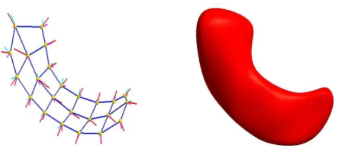
This data consists of 82 m-rep models (of Hippocampi), 56 of which are from schizophrenic individuals and the remaining 26 are from healthy control individuals (see Styner et al. (2004)). Each of these models have 24 medial atoms, placed in a 8_×3 lattice (see Fig. 3.3).

Figure 3.3: Left: M-rep sheet of a hippocampus with the 24 medial atoms. Right: Surface rendering of the m-rep model.

We conduct the simulation study in the following way. For each run we randomly remove five data points from the population of 82 and train our classifiers on the remaining 77 data points. For each such population we consider several values of the cost parameter λ (λ = 15k_{, k} _{= 0}_,₁_{, . . . ,}_{7) for ITanSVM, MSVM and TSVM. GMD} does not depend onλ. After training we test the classifiers by classifying the five test data points. Aggregating over several simulated replications, the training error and the cross-validation error are calculated.

(44)

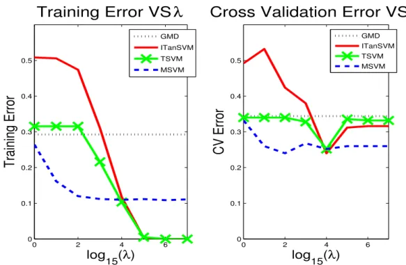
Fig. 3.4 shows the performance (training error (left panel) and cross-validation error(right panel)) of the different methods.

0 2 4 6

0 0.1 0.2 0.3 0.4 0.5

Training Error VS

λ

log₁₅(λ)

Training Error

GMD ITanSVM TSVM MSVM

0 2 4 6

0 0.1 0.2 0.3 0.4 0.5

Cross Validation Error VS

λ

log₁₅(λ)

CV Error

Figure 3.4: Left: Training errors against costlog₁₅λ. Right: Cross-validation errors against cost log₁₅λ. Cross-validation error for MSVM is robust to the choice of λ.

(45)

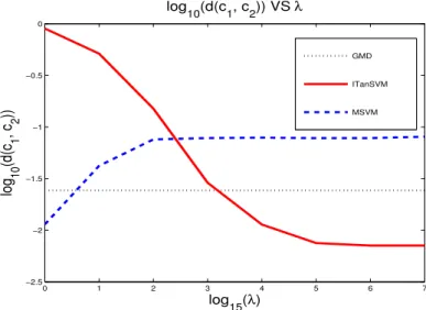
The MSVM algorithm suggests that with increasing λ the distance between c1 and c2 should increase (see equation 3.22). We monitor this tendency by plotting

d(c1, c2) against λ for MSVM, and for ITanSVM and GMD in order to compare the behavior of the solutions. Note that TSVM cannot be compared here since there are no control points involved. Fig. 3.5 plots log₁₀(d(c1, c2)) against log15λ.

0 1 2 3 4 5 6 7

−2.5 −2 −1.5 −1 −0.5 0

log₁₀(d(c₁, c₂)) VS λ

log₁₅(λ)

log 10

(d(c

1

, c 2

))

GMD ITanSVM MSVM

Figure 3.5: log₁₀(d(c1, c2)) against cost log15λ. The distance between the MSVM control points increases with increasing λ, as suggested by the problem formulation (equation 3.22).

Fig. 3.5 verifies that the solution of the MSVM algorithm behaves as expected: the distance betweenc1 andc2increases with increasingλ. The behavior of the ITanSVM solution is just the opposite. This behavior may be consistent with overfitting.

An important part of this study is to find out whether the classification rules under consideration give meaningful directions of difference between the classes. In the context of the given problem, the rule that best shows the structural change in the hippocampus is the most valuable. The structural change captured by each method is shown in Figure 3.6. For each classification rule (at the λ which has the least cross-validation error), we project the data points on to direction of separation. The mean of the projected data is calculated. The projected data points with the lowest and highest projection scores give the extent of structural change captured by

(46)

the separating direction. The objects in the left are the projected shapes with lowest score, and on the right, with the highest score. The color map shows the surface distance maps of the mean (of projected data points) and projected shapes. Red, green, and blue are inward distance, zero distance, and outward distance respectively.

Projected Patient Extreme Projected Control Extreme

GMD

TSVM

ITanSVM

MSVM

Figure 3.6: Diagram showing the structural change captured by the different methods. Red, green, and blue are inward distance, zero distance, and outward distance respectively.

(47)

conclude that MSVM provides the best balance between classifying performance and capturing changes in the shapes. Recall, that MSVM is the only method discussed here which works intrinsically on the manifold (and not on a tangent plane, like TSVM and ITanSVM) and this can be attributed to its desirable properties of good classification and informative separating direction.

3.3.4.2 Application to Generated Ellipsoid Data

This data consists of 25 m-rep models of generated distorted ellipsoids. They are simulated by randomly introducing a bending, twisting and tapering of an ellipsoid. We divide them into two groups, a group of 11 with negative twisting parameter and another group of 14 with positive twisting parameter. For our reference we call them the control group and the patient group respectively. Each of these models have 21 medial atoms, placed in a 7_×3 lattice (see Fig. 3.7).

m−rep sheet of a

deformed ellipsoid surface rendering of the m−rep model

Figure 3.7: Left: M-rep sheet of one of the simulated distorted ellipsoids used in our study. It has 21 medial atoms. Right: Surface rendering of the m-rep model.

As in the Hippocampi data set, we compare the performance of the different methods. The values of λ considered are the same as before. Instead of leaving five data points for each simulation, we leave out 3 data points in this case.

Fig. 3.8 shows the performance (training error (left panel) and cross-validation error(right panel)) of the different methods.

(48)

0 2 4 6 0 0.05 0.1 0.15 0.2 0.25 0.3 0.35 0.4 0.45

0.5

Training Error VS

λ

log₁₅(λ)

Training Error

0 2 4 6

0 0.05 0.1 0.15 0.2 0.25 0.3 0.35 0.4 0.45 0.5

Cross Validation Error VS

λ

log₁₅(λ)

CV Error

Figure 3.8: Left: Training Errors against log₁₅λ. Right: cross validation Errors against cost log₁₅λ. From the cross validation errors, none of the methods seem to overfit. MSVM is least sensitive to choice of λ.

MSVM (at λ= 15,154_{) has cross validation error very close to the lowest among} all the methods. Just as in the Hippocampus data set, the MSVM seems to be the least sensitive to high values of λ. But unlike the hippocampus data set, the cross validation errors of ITanSVM and TSVM do not increase with large λ. It seems for this dataset, these two methods are not overfitting. This can be attributed to the fact that the modes of noise component in this data set are far less than what we have in the real data set of hippocampi.

(49)

Projected Patient Extreme Mean of Projections Projected Control Extreme

TSVM

ITanSVM

MSVM

Figure 3.9: Structural change shown by TSVM, ITanSVM and MSVM. MSVM captures the true mode of difference (twisting), while TSVM and ITanSVM shows tapering/shrinking effect at the ends.

Again, MSVM seems to be bringing out the best balance of classifying power and capturing of separating features. Though, in this case, ITanSVM and TSVM do not seem to be overfitting, they fail to capture the true mode of change. This example again shows that MSVM, by virtue of its formulation (working on the manifold), captures the nonlinear modes of variation better than methods like ITanSVM and TSVM.

3.4 DWD on Manifolds

In this section, we introduce two approaches to extend DWD to manifold data. The following subsection reviews the standard DWD method.

(50)

3.4.1 A Brief Overview of Distance Weighted Discrimination

(DWD)

The DWD method, developed by Marron et al. (2004) is an improvement upon the Support Vector Machine in HDLSS contexts. For a recent application of DWD to microarray gene expression analysis, see Benito et al.(2004). Suppose two classes are separable, which is very likely for HDLSS data. Again, suppose the separating hyperplane is f(x) = wT_x₊_b_{. DWD finds the hyperplane that minimizes the sum of} the inverse distances. This gives larger influence to those points which are close to the hyperplane relative to the points that are farther away from the hyperplane (unlike SVM, where only the points closest to the separating hyperplane have important influence). For separable classes, the DWD method is the solution of the following optimization problem,

minimizew,bPn_i=1 1 ri

subject toyif(xi)≥0; i= 1, . . . , n, (3.24)

where ri is the distance of xi from the separating hyperplane. As shown in Figure 3.10, DWD finds a hyperplane (green) to separate the two classes (blue circles and red pluses) as well as possible, in the sense of minimizing the sum of the inverse distances from the samples to the hyperplane. The normal to the hyperplane is called the DWD separating direction. The computation of this hyperplane can be formulated as a Second-Order Cone Programming (SOCP) problem and is solved using the software package SDPT3 (for Matlab), which is web-available at Toh et al.

(2006).

(51)

Figure 3.10: DWD hyperplane (broken green line) to separate two classes, represented by crosses and pluses. The purple vector is the DWD direction of separation.

3.4.2 Iterative Tangent Plane DWD (ITanDWD)

In this subsection, we generalize DWD to manifold data by implementing standard DWD on multiple tangent planes, which are carefully chosen by an iterative approach. The algorithm is the same as proposed for ITanSVM in Section 3.3.2, except for the fact that in step 2, instead of SVM, the standard DWD method (described in 3.4.1) is implemented. The resulting method is called Iterative Tangent Plane DWD or ITanDWD.

3.4.3 The Manifold DWD (MDWD) method

Analogous to the ITanSVM method, ITanDWD also works by continual approx-imation of the data by projections on to the tangent plane. This makes ITanDWD unappealing. MDWD aims to be the first approach where all calculations are done on the manifold. Following the framework of Section 3.4.1, MDWD determines a pair of control points that minimizes the sum of the inverse distances from the training data to the separating boundary. The mathematical formulation of the method and the resulting optimization problem are given below.

(52)

As given in equation (3.1), the decision function fc1,c−1(x) is

fc1,c−1(x) = d 2₍_c

−1, x)−d2(c1, x)

The zero level set of fc1,c−1(·) defines the separating boundary H(c1, c−1) for a given pair (c1, c−1). We would like to solve for some ˜c1 and ˜c−1 such that

( ˜c1,c˜−1) = argmin c1,c−1

n

X

i=1

1

d(xi, H(c1, c−1))

(3.25)

In other words, we want to minimize the sum of the inverse distances from the training data to the separating boundary. Recall, from Chapter 2, that as in the classical SVM literature, we denoteyi to be the class label taking values -1 and 1.

By Lemma 3.1.1, in Euclidean space, note that the distance of any point x from the separating boundary H(c1, c−1) is

d(x, H(c1, c−1)) =

fc1,c−1(x) 2d(c1, c−1)

(3.26)

Therefore, for a separable training set (see Section 3.1), using (3.3) and (3.12), we can write the distance from the training points to the separating surface as

d(x, H(c1, c−1)) =

yfc1,c−1(x) 2d(c1, c−1)

, (3.27)

wherey=_±1 is the class label forx. Relation (3.27) will be used as an approximation that is reasonable for data on manifolds lying in a small (convex) neighborhood as this is directly computable for manifold data. Then, using (3.27) in (3.25) we would like to solve for some ˜c1 and ˜c−1 such that

( ˜c1,˜c−1) = argmin c1,c−1

n

X

i=1

2d(c1, c−1)

yifc1,c−1(xi)

(53)

Now, in order that the training points are correctly classified by H(c1, c−1), the following constraints should be satisfied:

∀i= 1. . . n,

yif(xi) ≥ 0

⇒ −yi{d2(xi, c−1)−d2(xi, c1)} ≤ 0 (3.29)

⇒hi ≤ 0

where hi =−yi{d2(xi, c−1)−d2(xi, c1)}.

Combining the constraints (hi < 0 ∀ i = 1. . . n) with (3.28), the optimization problem becomes

min c1,c−1

n

X

i=1

2d(c1, c−1)

yifc1,c−1(xi)

s.t. hi ≤0 (3.30)

Rather than solving the constrained optimization problem in (3.30), we consider the penalized minimization problem as defined below:

Minimize

gλ(c1, c−1) = n

X

i=1

d(c1, c−1)

yifc1,c−1(xi) + λ

n

X

i=1 (hi)+

or,

gλ(c1, c−1) = n

X

i=1

d(c1, c−1)

yi{d2(xi, c−1)−d2(xi, c1)} +λ n n X i=1

−yi{d2(xi, c−1)−d2(xi, c1)}

+ (3.31)

where λ is the penalty for violating the constraints given by (3.29).

Equation (3.31) gives the function to be minimized in the separable case. Note that the second term in (3.31) penalizes misclassification. In the non-separable case, the form of the function gλ(c1, c−1) to be minimized is given by:

gλ(c1, c−1) =

n

X

i: correctly classified

d(c1, c−1)

yi{d2(xi, c−1)−d2(xi, c1)} + + λ n n X i=1

−yi{d2(xi, c−1)−d2(xi, c1)}

+

(3.32)

(54)

or,

gλ(c1, c−1) = n

X

i=1

d(c1, c−1)

yi{d2(xi, c−1)−d2(xi, c1)}

+ + λ

n

X

i=1

−yi{d2(xi, c−1)−d2(xi, c1)}

+ (3.33)

A gradient descent approach was attempted to solve the above optimization prob-lem, but serious difficulties were encountered. Fig. 3.11 shows the MDWD objective

0 0.5 1 1.5 2 2.5

x 10−5

0 0.2 0.4 0.6 0.8 1 1.2 1.4 1.6 1.8

2x 10

5

stepsize (t)

MDWD objective function

Figure 3.11: Figure showing the discontinuous nature of the MDWD objective function as a function of the step size along the negative gradient direction.

function as a function of the step size along the negative gradient direction (with respect to c₋1). Note that the curve has several ‘spikes’, which indicates that the objective function is discontinuous at several points. This phenomenon prevents the negative gradient descent approach from working properly. The discontinuities are due to the denominator in the first term of the objective function given in Eq. (3.33). As soon as one of the misclassified points becomes properly classified, the denominator assumes a very small value and thus the objective function explodes.

(55)

ITanDWD and compare them with their SVM counterparts.

3.4.4 Results

In this section, we compare the performance of ITanDWD, TDWD, ITanSVM and TSVM. First, the real data set of hippocampi is revisited. The training errors and cross validation errors are calculated the same way as in Section 3.3.4.

3.4.4.1 Application To Hippocampi Data

Fig. 3.12 shows the performance (training error (left panel) and cross-validation error(right panel)) of the different methods. We note that the training errors of all

0 2 4 6

0 0.1 0.2 0.3 0.4 0.5

Training Error VS λ

log₁₅(λ)

Training Error

GMD ITanDWD TDWD ITanSVM TSVM

0 2 4 6

0 0.1 0.2 0.3 0.4 0.5

Cross Validation Error VS λ

log₁₅(λ)

CV Error

GMD ITanDWD TDWD ITanSVM TSVM

Figure 3.12: Comparison of methods for Hippocampus data. Left: Training errors against cost log₁₅λ. Right: Cross-validation errors against cost log₁₅λ. TDWD and ITanDWD have lower cross validation errors than their SVM counterparts.

the methods go to zero for higher values of λ. The cross validation errors of both TDWD and ITanDWD are less than their SVM counterparts (for higher values of

λ _≥154_{). This can be attributed to the fact that DWD is known to be more robust} to noise, especially in HDLSS situations. In fact, Figure 3.13 suggests that structural change shown by TDWD and ITanDWD are stronger than their SVM counterparts.

(56)

Projected Patient Extreme Projected Control Extreme

TDWD

ITanDWD

TSVM

ITanSVM

Figure 3.13: Diagram showing the structural change captured by the different methods. Red, green, and blue are inward distance, zero distance, and outward distance respectively. TDWD and ITanDWD capture stronger changes than their SVM counterparts.

3.4.4.2 Application To Generated Ellipsoid Data

Fig. 3.14 shows the performance (training error (left panel) and cross-validation error(right panel)) of the different methods. We note that the performances of TDWD and TSVM are very similar, while ITanDWD and ITanSVM are similar. It appears that relative to ITanSVM, ITanDWD is more robust to the choice of higher values of λ (the cross validation error for ITanDWD remains low for λ _≥ 154 _while that of ITanSVM increases).

Classification on manifolds

Classification on Manifolds

ABSTRACT

ACKNOWLEDGEMENTS

CONTENTS

LIST OF FIGURES

CHAPTER 1

Introduction

1.1

Motivation

1.2

Overview of Chapters

1.3

The Medial Locus and M-reps

1.3.1

Riemannian metric, Geodesic curve, Exponential and

Log maps

1.4

Statistical Methods on M-reps and on General

Manifolds

CHAPTER 2

Overview of Classification

2.1

The Problem of Classification

2.2

Popular Methods of Classification

2.3

Value Added by Working on Manifolds

2.3.1

Importance of Geodesic Distance on Manifolds

2.3.2

Choice of base point for Euclidean Classification on the

Tangent Plane

2.3.3

Validity and Interpretability of Projections

CHAPTER 3

Classification on Manifolds

3.1

Control Points and the General Classification

Rule

3.1.1

The Implied Separating Surface and Direction of

Sep-aration

3.1.2

Choice of Control Points

3.2

The Geodesic Mean Difference (GMD) Method

3.3

Support Vector Machine on Manifolds

3.3.1

A Brief Overview of Support Vector Machine (SVM)

3.3.2

Iterative Tangent Plane SVM (ITanSVM)

3.3.3

The Manifold SVM (MSVM) method

3.3.4

Results

Training Error VS

λ

Training Error

Cross Validation Error VS

λ

CV Error

Training Error VS

λ

Training Error

Cross Validation Error VS

λ

CV Error

3.4

DWD on Manifolds

3.4.1

A Brief Overview of Distance Weighted Discrimination

(DWD)

3.4.2

Iterative Tangent Plane DWD (ITanDWD)

3.4.3

The Manifold DWD (MDWD) method

3.4.4

Results