Cover Page
The handle
http://hdl.handle.net/1887/21949
holds various files of this Leiden University
dissertation.
Author
: Rahmati, Alireza
Title
:
Simulating the cosmic distribution of neutral hydrogen and its connection with
galaxies
S
neutral hydrogen
and
its connection with galaxies
ISBN978–9–46–191899–4
Cover by A. Rahmati
Front: The column density distribution of neutral hydrogen in a photoshoped
simulated galaxy. This design is motivated by the main findings of Chapter 4.
Back:Ancient constellations as published inThe book of fixed starsby the famous Iranian astronomer, Abd al-Rahman al-Sufi in 964 A.D. This highly influential book has been reproduced numerous times during the last millennium. The illustrations used for the design of the back-cover are taken from a version pro-duced in 1430-1440 A.D. in Samarkand (Uzbekistan), which is accessible through the following link:
S
neutral hydrogen
and
its connection with galaxies
P
roefschrift
ter verkrijging van
de graad van Doctor aan de Universiteit Leiden, op gezag van de Rector Magnificus prof. mr. C. J. J. M. Stolker,
volgens besluit van het College voor Promoties te verdedigen op dinsdag 15 oktober 2013
klokke 11:15 uur
door Alireza Rahmati geboren te Qom, Iran
Promotiecommissie
Promotor: Prof. dr. J. Schaye
Overige leden: Prof. dr. M. Franx
Dr. A. H. Pawlik (Max-Planck Institute for Astrophysics) Prof. dr. S. F. Portegies Zwart
Prof. dr. J. X. Prochaska (University of California, Santa Cruz) Prof. dr. H. J. A. Röttgering
T
C
1 Introduction 1
1.1 Current standard model for galaxy formation and evolution . . . . 2
1.1.1 Cosmology: the backbone of galaxy formation . . . 2
1.1.2 Main physical processes that drive galaxy evolution . . . . 3
1.2 Neutral hydrogen in galactic ecosystems . . . 4
1.3 Simulations . . . 6
1.3.1 Cosmological hydrodynamical simulations . . . 6
1.3.2 Radiative transfer . . . 8
1.3.3 Radiative transfer withTRAPHIC . . . 10
1.4 This thesis . . . 11
References . . . 13
2 On the evolution of theHicolumn density distribution in cosmological simulations 15 2.1 Introduction . . . 16
2.2 Simulation techniques . . . 18
2.2.1 Hydrodynamical simulations . . . 18
2.2.2 Radiative transfer withTRAPHIC . . . 19
2.2.3 Ionizing background radiation . . . 22
2.2.4 Recombination radiation . . . 26
2.2.5 The Hicolumn density distribution function . . . 26
2.2.6 Dust and molecular hydrogen . . . 27
2.3 Results . . . 30
2.3.1 Comparison with observations . . . 30
2.3.2 The shape of the HiCDDF . . . 34
2.3.3 Photoionization rate as a function of density . . . 36
2.3.4 The roles of diffuse recombination radiation and collisional ionization atz=3 . . . 39
2.3.5 Evolution . . . 41
2.4 Conclusions . . . 45
Acknowledgments . . . 46
References . . . 47
Appendix A: Photoionization rate as a function of density . . . 49
A1: Replacing the RT simulations with a fitting function . . . 49
A2: The equilibrium hydrogen neutral fraction . . . 50
Appendix B: The effects of box size, cosmological parameters and res-olution on the HiCDDF . . . 53
Appendix C: RT convergence tests . . . 53
C1: Angular resolution . . . 53
C2: The number of ViP neighbors . . . 53
C3: Direct comparison with another RT method . . . 55
Appendix D: Approximated processes . . . 56
TABLE OF CONTENTS
D2: Helium treatment . . . 57
3 The impact of local stellar radiation on theHicolumn density distribu-tion 59 3.1 Introduction . . . 61
3.2 Photoionization rate in star-forming regions . . . 63
3.3 Simulation techniques . . . 64
3.3.1 Hydrodynamical simulations . . . 64
3.3.2 Radiative transfer . . . 65
3.3.3 Ionizing background radiation and diffuse recombination radiation . . . 67
3.3.4 Stellar ionizing radiation . . . 68
3.4 Results and discussion . . . 70
3.4.1 The role of local stellar radiation in hydrogen ionization . . 70
3.4.2 Star-forming particles versus stellar particles . . . 76
3.4.3 Stellar ionizing radiation, its escape fraction and the buildup of the UVB . . . 79
3.4.4 The impact of local stellar radiation on the Hi column density distribution . . . 82
3.5 Discussion and conclusions . . . 87
Acknowledgments . . . 91
References . . . 91
Appendix A: Hydrogen molecular fraction . . . 93
Appendix B: Resolution effects . . . 94
B1: Limited spatial resolution at high densities . . . 94
B2: The impact of a higher resolution on the RT . . . 95
Appendix C: Calculation of the escape fraction . . . 97
4 Predictions for the relation between strongHiabsorbers and galaxies at redshift 3 99 4.1 Introduction . . . 100
4.2 Simulation techniques . . . 102
4.2.1 Hydrodynamical simulations . . . 102
4.2.2 Finding galaxies . . . 103
4.2.3 Finding strong Hiabsorbers . . . 103
4.2.4 Connecting Hiabsorbers to galaxies . . . 107
4.3 Results and discussion . . . 108
4.3.1 Spatial distribution of Hiabsorbers . . . 110
4.3.2 The effect of a finite detection threshold . . . 111
4.3.3 Distribution of Hiabsorbers relative to halos . . . 114
4.3.4 Resolution limit in simulations . . . 115
Break galaxies? . . . 124
4.4 Summary and conclusions . . . 126
Acknowledgments . . . 128
References . . . 128
Appendix A: Choosing the maximum allowed LOS Velocity difference . 131 Appendix B: Impact of feedback . . . 131
Appendix C: Impact of local stellar radiation . . . 134
Appendix D: Resolution tests . . . 135
5 Genesis of the dusty Universe: modeling submillimetre source counts 141 5.1 Introduction . . . 143
5.2 Model ingredients . . . 145
5.2.1 CLF atz=0 . . . 146
5.2.2 CLF evolution . . . 147
5.2.3 SED Model . . . 149
5.2.4 The algorithm . . . 150
5.3 850µm Observational Constraints . . . . 152
5.3.1 Observed 850µm source count . . . . 152
5.3.2 Redshift distribution of bright 850µm sources . . . . 153
5.4 Finding 850µm best-fit Model . . . . 154
5.4.1 The source count curve: Amplitude vs. Shape . . . 154
5.4.2 The luminosity evolution . . . 155
5.5 Other necessary model ingredients . . . 157
5.5.1 The 850µm best-fit model . . . . 159
5.6 Other wavelengths . . . 160
5.6.1 Long submm wavelengths: 850µm and 1100µm . . . . 162
5.6.2 SPIRE intermediate wavelengths: 500µm, 350µm and 250µm . . . . 164
5.6.3 Short wavelengths: 160µm and 70µm . . . . 165
5.6.4 A best-fit model for all wavelengths . . . 166
5.7 Discussion . . . 171
5.7.1 The implied evolution scenario for dusty galaxies . . . 171
5.7.2 Our best-fit model and previous models . . . 175
5.8 Conclusions . . . 177
Acknowledgments . . . 178
References . . . 179
Appendix A: Some numerical details . . . 181
Publications 183
1
I
ntroduction
For more than a millennium, we have been aware of the existence of a celes-tial small cloud in the constellation of Andromeda (al-Sufi,964), but it has been less than a century since we observed that the small cloud, which is commonly known to us as M31, is a spiral galaxy outside of our own Milky Way. In fact, al-most everything we know about M31 and other galaxies has been learned during the last century, thanks to the advent of large telescopes and new technologies. During the last few decades, theoretical models have helped us to make sense of the rapidly increasing wealth of data and have caused a revolution in our understanding of the Universe. In particular, as a result of advancements in nu-merical techniques and computational recourses, cosmological simulations have become an indispensable tool for probing the main processes involved in galaxy formation and evolution.
Introduction
1.1
Current standard model for galaxy formation and
evolution
The theory of galaxy formation is where the properties of the largest scales in the Universe meet the physics at tiny atomic scales. The huge dynamic range of the relevant scales spanned by the different physical entities (e.g., length, mass, time) that characterize galaxies, makes it a daunting task to model these complex systems. Despite the monstrous size of this problem, in principle, the formation and evolution of galaxies should be understandable in terms of the known physical laws. Using these physical laws to explain the observed trends among galaxies has been the main challenge of the theory of galaxy formation and evolution. As a result of the hard work of many great minds, we now have an understanding of how galaxies form and evolve, which can explain, with a good degree of accuracy, what we see in the Universe. However, as in other natural sciences, any progress in understanding galaxies reveals new puzzles to solve. As a result, there is (and there will be) a huge number of phenomena that we do not fully understand. In the following, I briefly review what I call the standardmodel of galaxy formation and evolution, which consists of ideas that glue together large sets of observed properties, and are commonly accepted by most experts who work in this field.
1.1.1
Cosmology: the backbone of galaxy formation
Cosmology serves as the backbone of galaxy formation by describing the physical laws that govern the formation and evolution of structures on large scales. In this context, the ΛCDM paradigm has enjoyed great success by
explaining a large number of observables, such as the temperature fluctu-ations in the radiation we receive from the early Universe (i.e., the Cosmic Microwave Background), the accelerated expansion of the Universe and the growth of structures. The constraints on the parameters of the ΛCDM
con-cordance cosmological model have been improving rapidly in recent years, thanks to precise observational experiments like the Cosmic Background Ex-plorer (COBE:Mather et al.,1990), the Wilkinson Microwave Anisotropy Probe (WMAP:Bennett et al., 2003;Spergel et al., 2003;Komatsu et al.,2011) and re-cently, the Planck satellite (Planck Collaboration et al.,2013). Based on the above mentioned measurements, and other experiments, we know that the vast major-ity of the energy densmajor-ity of the Universe is in the form of Dark Energy (i.e.,
Λ), which causes the accelerating expansion of the Universe. The rest consists
As the Universe expands, the separation between small scale density fluctu-ations increases. At the same time, the deviation between the density of fluc-tuations and the mean density of the Universe also increases. In other words, over-dense regions attract more matter at the expense of draining under-dense regions. When the density fluctuation (i.e.,∆ρ) is much smaller than the mean
density of the Universe (i.e.,∆ρ/ρ ≪1), its physical size increases with the
ex-pansion of the Universe as the magnitude of∆ρincreases (i.e., the linear regime).
There is, however, a turn-around when∆ρ/ρ ∼1, after which the physical size
of the fluctuation starts to decrease (i.e., the non-linear regime). The result of the latter stage is the formation of self-gravitating bound structures. Since the ma-jority of matter is in the form of collisionless dark matter, collapsing structures (i.e., dark mater haloes) are regularized through violent relaxation. On large scales and low over-densities, the baryonic matter is bound to the dark matter, which is the dominant gravitational actor. In the non-linear regime, however, baryons reveal their collisional nature and become shock heated to very high temperatures through the efficient conversion of gravitational energy into the internal energy of the baryonic gas, as it collapses into the inner parts of the gravitational potential wells. At this stage, the fate of baryons in the collapsed structures is significantly affected by the laws of small-scale atomic physics and related complex and collective processes like radiative cooling and star form-ation. At the same time, the large-scale evolution of structures continues and brings more matter into the collapsed structures and merges them.
1.1.2
Main physical processes that drive galaxy evolution
Despite the great success of the ΛCDM paradigm in explaining the invisible
side of galaxy formation by accurately predicting the formation and growth of dark matter haloes (e.g.,Zehavi et al.,2011;Heymans et al.,2013), the complex physical processes that control the evolution of gas and stars are far from un-derstood. To first order, the baryonic content of collapsing dark matter haloes, which is initially shock heated to high temperatures, loses its energy through ra-diative cooling. The conservation of angular momentum dictates the cooling gas to form a rotating disk as it looses energy and falls deeper into the potential well of the dark matter halo. The density of baryonic gas increases until the radiative cooling becomes inefficient and the gaseous disk approaches a quasi-equilibrium state. The small scale instabilities in the gaseous disk, however, continue to grow into dense molecular clouds which evolve and collapse to form stars.
Introduction
faster than stars with lower masses, end their lives dramatically in energetic ex-plosions (i.e., Supernovae; SNe) that inject huge amounts of energy into the ISM of their host galaxies, affecting subsequent star formation and launching large-scale galactic winds. In addition to energetic SNe explosions, radiation pressure from very luminous young stars removes gas from star-forming regions, and possibly makes a significant contribution to the launching of galactic winds.
The presence of very massive black holes, the end result of the death of very massive stars, causes more complications in our understanding of how galaxies evolve. Super-massive black holes, which are found at the centers of many (if not all) galaxies we see in the Universe, are very efficient in converting mass into energy. The huge amount of energy they inject into their host galaxies in different ways, changes their fate dramatically.
There is much solid observational evidence and there are strong theoretical arguments for the presence and importance of the above mentioned mechan-isms in the formation and evolution of galaxies. Understanding how they work individually and together to control the lives of galaxies at different epochs has been an active area of research during the last few decades, an area of research which is still vibrantly active due to its complexity.
1.2
Neutral hydrogen in galactic ecosystems
As mentioned above, galaxies are influenced on the one hand by the force of gravity, which forms haloes, brings fresh material into the already existing ha-loes and keeps baryonic and dark matter structures together, and on the other hand, by the feedback mechanisms that fight against the force of gravity and try to unbind structures. The interaction between these two fronts creates a complex ecosystem in and around galaxies, and imprints the history of galax-ies in the distribution of baryons around them (i.e., the circumgalactic medium; CGM). In this context, understanding the distribution of neutral hydrogen (HI) is of particular importance. The main reason for this is that Hiis the main fuel
for the formation of molecular clouds, the birth places of stars, which makes studying the distribution of Hiand its evolution crucial for our understanding
of various aspects of star formation.
and quasars at lower redshifts (e.g., Becker & Bolton, 2013). As a result, after reionization most hydrogen atoms are kept ionized by the UVB radiation they receive from all the ionizing sources they can see in the Universe.
The complexity of processes that set the ionization state of hydrogen depends on the Hicolumn density. At low Hi column densities (i.e., NHI .1017cm−2, corresponding to the so-called Lyman-α forest), hydrogen is highly ionized by the UVB radiation and largely transparent to the ionizing radiation. For these systems, the Hicolumn densities can therefore be accurately computed in the
optically thin limit. At higher Hicolumn densities (i.e., NHI &1017cm−2, cor-responding to the so-called Lyman Limit and Damped Lyman-α systems), the gas becomes optically thick and self-shielded. As a result, the ionization state of hydrogen in these systems is more sensitive to various radiative transfer effects such as self-shielding, shadowing and the fluctuations of the UVB radiation on small scales.
Studying the distribution of Hiis proven to be challenging. In the local
Uni-verse, the Hicontent of galaxies can be probed by observing 21-cm emission, but
at higher redshifts this will not be possible until the advent of significantly more powerful telescopes, such as the Square Kilometer Array1. At z .6, i.e., after reionization, the neutral gas can be probed through absorption signatures that are imprinted by the intervening Hisystems on the spectra of bright background
sources, such as quasars. The analysis of these absorption features provides an alternative probe of the distribution of matter at high redshifts, compared to studying the Universe through emission. The large distances that separate most absorbers from their background QSOs make it unlikely that there is a physical connection between them. This opens up a window to study an unbiased sample of matter that resides between us and the background QSOs.
Constraining the statistical properties of the Hidistribution has been the
fo-cus of many observational studies during the last few decades (e.g.,Tytler,1987; Kim et al., 2002; Péroux et al., 2005; O’Meara et al., 2007; Noterdaeme et al., 2009; Prochaska et al., 2009; O’Meara et al., 2013). Thanks to a significant in-crease in the number of observed quasars and improved observational tech-niques, more recent studies have extended these observations to both lower and higher Hicolumn densities and to higher redshifts. Therefore, it is important to
study the properties of the Hidistribution in cosmological simulations to better
understand the observed trends and to put them in the context of the standard theory of galaxy formation and evolution, which is the focus of this thesis. Once simulations agree with observations, one can use them to predict what future observations reveal. These predictions can be used to validate the underlying models in the simulations and to examine the importance of different processes that are relevant to the formation and evolution of galaxies, or in case of dis-agreement, to point us to necessary improvements.
Introduction
1.3
Simulations
Hydrodynamical simulations attempt to model complex baryonic interactions by combining various physically motivated and empirical ingredients. Modern state-of-the-art cosmological simulations of galaxy formation try to put together most of what we know about the astrophysical and cosmological processes that are shaping the Universe on different scales and they try to reproduce different observables.
In this context, the vital importance of radiation and radiative transfer (RT) processes for galaxy evolution in general, and for producing the Hidistribution
in particular, is evident. However, RT is often ignored or poorly approximated in the simulations. The main reason for this is the high dimensionality of the underlying calculation which makes RT an enormous computational challenge for cosmological simulations. Thanks to increasingly more powerful computers, and in the light of new algorithms, the accurate treatment of radiative effects is now becoming possible.
Since in this thesis we extensively use hydrodynamical simulations and RT, we will briefly discuss how they work.
1.3.1
Cosmological hydrodynamical simulations
Cosmological simulations calculate the evolution of the Universe by starting from an approximately uniform density of matter with small fluctuations on different scales. These fluctuations are set by the observed statistical properties of the fluctuations in the early stages of the Universe (i.e., the CMB). To be able to trace the evolution of the Universe numerically, different techniques are ad-opted to discretize the continuous distribution of matter into a finite number of resolution elements (e.g., particles). In addition, to keep the numerical calcu-lations tractable, one needs to adopt a finite volume which is assumed to be a representative sample of the whole Universe. Periodic boundary conditions can then be used which assume that the distribution of matter on scales beyond the extent of the simulation box is statistically similar to that inside it.
The gravitational interactions between all particles in the simulation are fol-lowed directly while the large-scale cosmological expansion of the Universe is accounted for by a change of coordinate system. Different techniques are used to accelerate the computation of the gravitational field without losing accuracy significantly. For instance, calculating the gravitational interaction between two groups of particles that are far away from each other (compared to the typical distances between the particles in each group) is possible even if we neglect the small scale distribution of the group members and replace the whole group with a single gravitationally interacting element (see for an example the TreePM algorithm explained inBagla,2002).
neigh-boring resolution elements interact hydrodynamically. One of the most success-ful methods to simulate the evolution of the gas fluid is the smoothed particle hydrodynamic (SPH) technique which was introduced byGingold & Monaghan (1977) andLucy(1977). In the SPH prescription, the fluid is discretized into in-dividual particles that are smoothed. This means that the relevant properties of the fluid that are represented by each particle are distributed smoothly in space around the particle. Then, the value of each relevant quantity (in most cases only density), for any given position, is calculated by adding the contribution of all SPH particles that are close enough to have significant contributions. Then, the evolution of the fluid is calculated based on the known physical laws that affect the fluid, like the laws of mass, momentum and energy conservation.
By combining the gravitational and hydrodynamical forces, it is possible to start from small initial fluctuations and trace the evolution of dark matter and baryonic gas as the Universe evolves. As the formation of structure proceeds, the baryonic content of collapsing structures, which is initially shock heated, cools down due to radiative cooling. The radiative cooling is calculated in the simulations by including several important atomic processes. These processes are mainly sensitive to the density, temperature, the abundances of different elements (i.e., metallicity) and the properties of the radiation field. Because of the high-dimensionality of the equations that control the cooling, their net effect is included in the simulations using fitting functions and tables. Due to cooling, the density of baryons increases which further complicates the simulation of the evolution of baryons.
The limited spatial resolution of cosmological simulations, which is usually of the order of a kilo-parsec, is not enough to resolve the complex and multi-phase structure of the ISM. Because of this, an effective equation of state is often adopted to model the collective hydrodynamical properties of the ISM gas. This effective equation of state can also be used to prevent artificial fragmentation of dense gas on scales close to the resolution limit (Schaye & Dalla Vecchia,2008). As the gas density increases, the dense ISM should be converted into stars. Since it is not possible to simulate the complex process of star formation at kpc res-olution, simplified algorithms are used to convert gas into stars. These star formation prescriptions are often tuned to match the observed relation between the gas (column) density and star formation rate in real galaxies, on kpc scales (i.e., the Kenicutt-Schmidt relation;Kennicutt,1998).
The resolution elements (e.g., SPH particles) that satisfy the adopted star formation criteria are converted into stellar particles with typical masses of 105−106 M
⊙. In other words, each stellar particle in cosmological
Introduction
enough to explode as SNe, end their lives in dramatic explosions and heat up the gas which also launches high velocity flows that create large-scale galactic winds. All these processes, together with other complicated phenomena, are poorly understood and their detailed simulation requires much higher resolu-tion than what is affordable in current cosmological simularesolu-tions. Therefore, they are included in the simulations through approximate rules, similar to the form-ation of stars explained above, which are commonly known as sub-grid models. The sub-grid models in cosmological simulations try to incorporate our physical knowledge or observed empirical relations into simulations. Due to the large uncertainties, they are often tuned to produce the desired observables, such as the average star formation activity of the Universe or the stellar mass function at different epochs. Because of the complexity of how different subgrid mod-els work individually and in combination, implementing them reliably in the simulations and understanding how they regulate galaxies is an active area of research.
By combining all the above mentioned ingredients (i.e., gravity, hydrodynam-ics and subgrid models), it is possible to start from initial conditions that are set by cosmological observations, and to simulate the formation and evolution of galaxies and the cosmic distribution of gas.
1.3.2
Radiative transfer
In addition to hydrodynamical and gravitational interactions, radiation plays an important role in shaping the cosmos as we see it. The interaction between light and matter has important consequences for the evolution of structures across a range of different scales. While the radiation pressure close to stars, and perhaps on galactic scales, changes the dynamics of the gas, the UVB radiation, which is the superposition of radiation from large numbers of sources distributed on large scales, affects the cooling/heating of the baryons significantly. In addition, it is impossible to interpret the observations without understanding the rela-tion between the measured intensity of radiarela-tion and different phenomena that produce/affect photons.
Introduction
1.3.3
Radiative transfer with
TRAPHICBecause of the reasons mentioned above, RT is sensitive to a large number of variables which makes it computationally expensive. Various techniques have been developed to reduce the computational cost of the RT, mainly by adopting different simplifying assumptions. Among different methods,TRAPHIC (TRAns-port of PHotons In Cones;Pawlik & Schaye,2008,2011) is a unique RT method with several important advantages, as is explained below, for radiation trans-port in cosmological simulations that use the SPH prescription. Since we use SPH simulations in this work,TRAPHICis a natural choice to compute the RT. In the following we briefly review how photon transfer is done withTRAPHIC(see also Figure1.1).
TRAPHIC is an explicitly photon-conserving RT method designed to trans-port radiation directly on the irregular distribution of SPH particles. This means that unlike many RT methods that use coarse grids to simplify the calculations, TRAPHICexploits the full dynamic range that is available based on the underly-ing SPH simulation. Another challenge that RT methods face is the large num-ber of sources in cosmological simulations. The computational cost of most RT methods is proportional to the number of radiation sources, which poses a big challenge for cosmological RT simulations. TRAPHIC solves this problem by tracing photon packets inside a discrete number of cones which renders the computational cost of the RT independent of the number of radiation sources. The two above mentioned advantages make TRAPHIC particularly well-suited for RT calculation in cosmological density fields with a large dynamic range in densities and large numbers of sources.
The photon transport in TRAPHIC proceeds in two steps: the isotropic emission of photon packets by source particles and their subsequent direc-ted propagation on the irregular distribution of SPH particles. After sources emit photon packets isotropically to their neighbors, the photon packets travel along their propagation directions to neighboring SPH particles which are in-side their transmission cones. Transmission cones are regular cones with solid angle 4π/NTC and are centered on the propagation direction. The parameter NTC sets the angular resolution of the RT. The transmission cones are defined locally at the transmitting particle, and hence the angular resolution of the RT withTRAPHICis independent of the distance from the source.
It can happen that transmission cones do not contain any neighboring SPH particles. In this case, additional particles (virtual particles, ViPs) are placed inside the transmission cones to accomplish the photon transport. The ViPs, which enable the particle-to-particle transport of photons along any direction independently of the spatially inhomogeneous distribution of the particles, do not affect the SPH simulation and are deleted after the photon packets have been transferred.
number of sources. Photon packets received by each SPH particle are binned based on their propagation directions in NRC reception cones. Then, photon packets with identical frequencies that fall in the same reception cone are merged into a single photon packet with a new direction set by the luminosity-weighted sum of the directions of the original photon packets.
Photon packets are transported along their propagation direction until they reach the distance they are allowed to travel within the RT time step by the finite speed of light. At the end of each time step the ionization states of the particles are updated based on the number of absorbed ionizing photons.
By following the aforementioned steps, TRAPHIC calculates the radiation field in cosmological simulations and the ionization state of different species accurately (see Pawlik & Schaye, 2008, 2011). In this work, we mainly use TRAPHIC to calculate the ionization state of hydrogen by taking into account different sources of radiation.
1.4
This thesis
Observational studies are moving rapidly beyond studying only the stellar com-ponents of galaxies, towards probing the important but complex processes that affect the distribution of gas in and around galaxies. Hydrodynamical cosmo-logical simulations of galaxy formation are also improving rapidly by including better numerical techniques, more physically motivated and better-understood subgrid models and by using higher resolution. It is important, if not essential, to compare observations and simulations in order to improve our understanding of the observational results and to test/improve the simulations.
The neutral hydrogen distribution and its evolution is closely related to vari-ous aspects of star formation. This makes understanding and modeling the Hi
distribution critically important for studying galaxy evolution. The main focus of this thesis is therefore the study of the cosmic distribution of neutral hydro-gen using hydrodynamical cosmological simulations. To do this, we combine hydrodynamical cosmological simulations based on the OverWhelmingly Large Simulations (OWLS;Schaye et al.,2010) with accurate radiative transfer, and ac-count for different photoionizing processes.
In Chapter 2, we include the radiative transfer effects of the metagalactic
UVB radiation and diffuse recombination radiation for hydrogen ionization at redshiftsz=5−0. We focus on studying Hicolumn densitiesNHI >1016cm−2,
where RT effects can be important. By modeling more than 12 billion years of evolution of the Hidistribution, we show that the predicted Hicolumn density
distribution is in excellent agreement with observations and evolves only weakly from z = 5 to z = 0. We find that the UVB is the dominant source of Hi
Introduction
hydrogen fractions without RT. Given the difficulty of RT simulations, these fit-ting functions are particularly useful for the next generation of high resolution cosmological simulations.
Stars typically form at very high column densities, where the gas is self-shielded against the external ionizing radiation. This makes local stellar ra-diation an important source of ionization at these column densities. However, simulating the effect of ionizing stellar radiation for the large numbers of sources that are typical of cosmological simulations, is extremely challenging. As a res-ult, different studies have found different (and often inconclusive) results regard-ing the importance of local stellar radiation on the Hidistribution. InChapter
3, we tackle this problem by combining cosmological simulations with RT using
TRAPHIC, which is designed to handle large numbers of sources efficiently. We simulate the ionizing radiation from stars together with the UVB and recombin-ation radirecombin-ation. We show that the local stellar radirecombin-ation can significantly change the Hicolumn density distribution at column densities relevant for the so-called
Damped Lyα (DLA) and Lyman-Limit (LL) systems. We also show that the main source of disagreement between previous works is insufficient resolution, a problem we solve by using star-forming particles as ionizing sources. We also show that the absence of a fully resolved ISM in cosmological simulations is a bottle-neck for modelling the properties of strong DLAs (i.e.,NHI≥1021cm−2). Strong Hiabsorbers, such as DLAs, are likely to be representative of the cold
gas in, or close to, the ISM in high-redshift galaxies. Because of this, they provide a unique opportunity to define an absorption-selected galaxy sample and to study the ISM, particularly at the early stages of galaxy formation. However, because observational studies are limited by the small number of known strong Hi absorbers and are missing low-mass galaxies in surveys for their
counter-parts in emission, it is very difficult to probe the relation between Hiabsorbers
and their host galaxies observationally and we have to resort to cosmological simulations to help us understand the link between the two. InChapter 4, we
use the hydrodynamical cosmological simulations that we have shown to match the Hiobservations very well (see Chapter 2), to study the link between strong
Hisystems and galaxies at z= 3. We show that most strong Hiabsorbers are
associated with low-mass galaxies too faint to be detected in current observa-tions. We demonstrate, however, that our predictions are in good agreement with the existing observations. We show that there is a strong anti-correlation between the column density of strong Hi absorbers and the impact
paramet-ers that connect them to their closest galaxies. We also investigate correlations between the column density of strong Hi absorbers and different properties of
their associated galaxies.
of individual distant infrared galaxies a daunting task. Significant information about the evolution and statistical properties of these objects is encoded in the surface density of sources as a function of brightness (i.e., the source count). InChapter 5, we present a model for the evolution of dusty galaxies, constrained by the 850µmsource counts and redshift distribution. We use a simple formal-ism for the evolution of the luminosity function and the color distribution of infrared galaxies. Using a novel algorithm for calculating the source counts, we analyze how individual free parameters in the model are constrained by ob-servational data. The model is shown to successfully reproduce the observed source count and redshift distributions at wavelengths 70µm.λ.1100µm, and to be in excellent agreement with the most recentHerschelandSCUBA 2results.
References
al-Sufi, Abd al-Rahman,Book of Fixed Stars, 964, Isfahan, Iran Bagla, J. S. 2002, Journal of Astrophysics and Astronomy, 23, 185 Becker, G. D., & Bolton, J. S. 2013, arXiv:1307.2259
Bennett, C. L., Halpern, M., Hinshaw, G., et al. 2003, ApJS, 148, 1 Gingold, R. A., & Monaghan, J. J. 1977, MNRAS, 181, 375
Heymans, C., Grocutt, E., Heavens, A., et al. 2013, MNRAS, 432, 2433 Kennicutt, R. C., Jr. 1998, ApJ, 498, 541
Kim, T.-S., Carswell, R. F., Cristiani, S., D’Odorico, S., & Giallongo, E. 2002, MNRAS, 335, 555
Komatsu, E., Smith, K. M., Dunkley, J., et al. 2011, ApJS, 192, 18 Lucy, L. B. 1977, AJ, 82, 1013
Mather, J. C., Cheng, E. S., Eplee, R. E., Jr., et al. 1990, ApJL, 354, L37
Noterdaeme, P., Petitjean, P., Ledoux, C., & Srianand, R. 2009, A&A, 505, 1087 O’Meara, J. M., Prochaska, J. X., Burles, S., et al. 2007, ApJ, 656, 666
O’Meara, J. M., Prochaska, J. X., Worseck, G., Chen, H.-W., & Madau, P. 2013, ApJ, 765, 137
Pawlik, A. H., & Schaye, J. 2008, MNRAS, 389, 651 Pawlik, A. H., & Schaye, J. 2011, MNRAS, 412, 1943
Péroux, C., Dessauges-Zavadsky, M., D’Odorico, S., Sun Kim, T., & McMahon, R. G. 2005, MNRAS, 363, 479
Planck Collaboration, Ade, P. A. R., Aghanim, N., et al. 2013, arXiv:1303.5076 Prochaska, J. X., Worseck, G., & O’Meara, J. M. 2009, ApJL, 705, L113
Schaye, J., & Dalla Vecchia, C. 2008, MNRAS, 383, 1210
Schaye, J., Dalla Vecchia, C., Booth, C. M., et al. 2010, MNRAS, 402, 1536 Spergel, D. N., Verde, L., Peiris, H. V., et al. 2003, ApJS, 148, 175
Tytler, D. 1987, ApJ, 321, 49
2
O
n the evolution of the
H
i
column density distribution in
cosmological simulations
We use a set of cosmological simulations combined with radiative transfer calculations to investigate the distribution of neutral hydrogen in the post-reionization Universe. We assess the contributions from the metagalactic ion-izing background, collisional ionization and diffuse recombination radiation to the total ionization rate at redshiftsz=0−5. We find that the densities above which hydrogen self-shielding becomes important are consistent with analytic calculations and previous work. However, because of diffuse recombination ra-diation, whose intensity peaks at the same density, the transition between highly ionized and self-shielded regions is smoother than what is usually assumed. We provide fitting functions to the simulated photoionization rate as a function of density and show that post-processing simulations with the fitted rates yields results that are in excellent agreement with the original radiative transfer cal-culations. The predicted neutral hydrogen column density distributions agree very well with the observations. In particular, the simulations reproduce the remarkable lack of evolution in the column density distribution of Lyman limit and weak damped Lyαsystems below z = 3. The evolution of the low column density end is affected by the increasing importance of collisional ionization with decreasing redshift. On the other hand, the simulations predict the abundance of strong damped Lyαsystems to broadly track the cosmic star formation rate density.
Alireza Rahmati, Andreas H. Pawlik, Milan Raiˇcevi`c, Joop Schaye
On the evolution of theHiCDDF
2.1
Introduction
A substantial fraction of the interstellar medium (ISM) in galaxies consists of atomic hydrogen. This makes studying the distribution of neutral hydrogen (Hi) and its evolution crucial for our understanding of various aspects of star
formation. In the local universe, the Hicontent of galaxies is measured through
21-cm observations, but at higher redshifts this will not be possible until the advent of significantly more powerful telescopes such as the Square Kilometer Array1. However, at z . 6, i.e., after reionization, the neutral gas can already be probed through the absorption signatures imprinted by the intervening Hi
systems on the spectra of bright background sources, such as quasars (QSOs). The early observational constraints on the Hi column density distribution
function (Hi CDDF hereafter), from quasar absorption spectroscopy at z . 3, were well described by a single power-law in the rangeNHI ∼1013−1021cm−2 (Tytler, 1987). Thanks to a significant increase in the number of observed quasars and improved observational techniques, more recent studies have ex-tended these observations to both lower and higher Hi column densities and
to higher redshifts (e.g., Kim et al., 2002; Péroux et al., 2005; O’Meara et al., 2007; Noterdaeme et al., 2009; Prochaska et al., 2009; Prochaska & Wolfe, 2009; O’Meara et al., 2013; Noterdaeme et al., 2012). These studies have revealed a much more complex shape which has been described using several different power-law functions (e.g.,Prochaska et al.,2010;O’Meara et al.,2013).
The shape of the HiCDDF is determined by both the distribution and
ion-ization state of hydrogen. Consequently, determining the distribution function of Hicolumn densities requires not only accurate modeling of the cosmological
distribution of gas, but also radiative transfer (RT) of ionizing photons. As a starting point, the Hi CDDF can be modeled by assuming a certain gas
pro-file and exposing it to an ambient ionizing radiation field (e.g.,Petitjean et al., 1992;Zheng & Miralda-Escudé,2002). Although this approach captures the ef-fect of self-shielding, it cannot be used to calculate the detailed shape and nor-malization of the Hi CDDF which results from the cumulative effect of large
numbers of objects with different profiles, total gas contents, temperatures and sizes. Moreover, the interaction between galaxies and the circum-galactic me-dium through accretion and various feedback mechanisms, and its impact on the overall gas distribution are not easily captured by simplified models. There-fore, it is important to complement these models with cosmological simulations that model the evolution of the large-scale structure of the Universe and the formation of galaxies.
The complexity of the RT calculation depends on the Hi column density.
At low Hi column densities (i.e., NHI . 1017cm−2, corresponding to the so-called Lyman-α forest), hydrogen is highly ionized by the metagalactic ultra-violet background radiation (hereafter UVB) and largely transparent to the
izing radiation. For these systems, the Hi column densities can therefore be
accurately computed in the optically thin limit. At higher Hi column densities
(i.e.,NHI &1017cm−2, corresponding to the so-called Lyman Limit and Damped Lyman-αsystems), the gas becomes optically thick and self-shielded. As a result, the accurate computation of the Hi column densities in these systems requires
precise RT simulations. On the other hand, at the highest Hi column densities
where the gas is fully self-shielded and the recombination rate is high, non-local RT effects are not very important and the gas remains largely neutral. At these column densities, the hydrogen ionization rate may, however, be strongly affected by the local sources of ionization (Miralda-Escudé,2005;Schaye,2006; Rahmati et al., 2013). In addition, other processes like H2 formation (Schaye, 2001b; Krumholz et al., 2009; Altay et al., 2011) or mechanical feedback from young stars and / or AGNs (Erkal et al., 2012), can also affect the highest Hi
column densities.
Despite the importance of RT effects, most of the previous theoretical works on the Hicolumn density distribution did not attempt to model RT
ef-fects in detail (e.g., Katz et al.,1996;Gardner et al., 1997; Haehnelt et al.,1998; Gardner et al.,2001;Cen et al.,2003;Nagamine et al.,2004,2007). Only very re-cent works incorporated RT, primarily to account for the attenuation of the UVB (Razoumov et al., 2006; Pontzen et al.,2008; Fumagalli et al., 2011; Altay et al., 2011;McQuinn et al.,2011) and found a sharp transition between optically thin and self-shielded gas that is expected from the exponential nature of extinction. The aforementioned studies focused mainly on redshiftsz=2−3, for which observational constraints are strongest, without investigating the evolution of the Hidistribution. They found that the HiCDDF in current cosmological
simula-tions is in reasonable agreement with observasimula-tions in a large range of Hicolumn
densities. Only at the highest Hicolumn densities (i.e., NHI & 1021cm−2) the agreement is poor. However, it is worth noting that the interpretation of these Hisystems is complicated due to the complex physics of the ISM and ionization
by local sources. Moreover, the observational uncertainties are also larger for these rare highNHI systems.
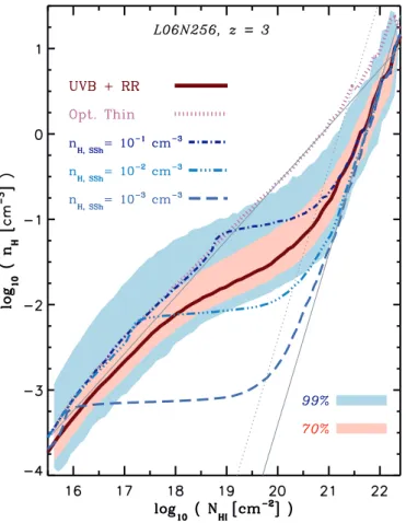
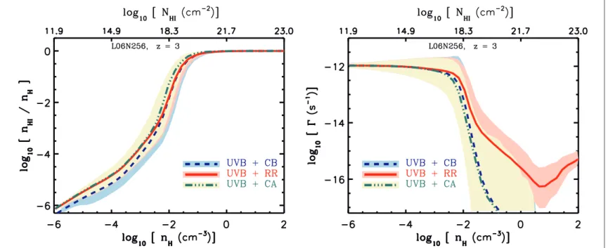
In this chapter, we investigate the cosmological Hidistribution and its
evolu-tion during the last&12 billion years (i.e.,z.5). For this purpose, we use a set of cosmological simulations which include star formation, feedback and metal-line cooling in the presence of the UVB. These simulations are based on the Overwhelmingly Large Simulations (OWLS) presented in Schaye et al. (2010). To obtain the HiCDDF, we post-processed the simulations with RT, accounting
for both ionizing UVB radiation and ionizing recombination radiation (RR). In contrast to previous works, we account for the impact of recombination radi-ation explicitly, by propagating RR photons. Using these simulradi-ations we study the evolution of the Hi CDDF in the range of redshiftsz = 0−5 for column
densities NHI &1016cm−2. We discuss how the individual contributions from the UVB, RR and collisional ionization to the total ionization rate shape the Hi
On the evolution of theHiCDDF
The structure of this chapter is as follows. In §2.2we describe the details of the hydrodynamical simulations and of the RT, including the treatment of the UVB and recombination radiation. In §2.3we present the simulated HiCDDF
and its evolution and compare it with observations. In the same section we also discuss the contributions of different ionizing processes to the total ionization rate and provide fitting functions for the total photoionization rate as a function of density which reproduce the RT results. Finally, we conclude in §2.4.
2.2
Simulation techniques
2.2.1
Hydrodynamical simulations
We use density fields from a set of cosmological simulations performed using a modified version of the smoothed particle hydrodynamics codeGADGET-3(last described in Springel, 2005). The subgrid physics is identical to that used in the reference simulation of the OWLS project (Schaye et al., 2010). Star form-ation is pressure dependent and reproduces the observed Kennicutt-Schmidt law (Schaye & Dalla Vecchia, 2008). Chemical evolution is followed using the model of Wiersma et al. (2009a), which traces the abundance evolution of el-even elements by following stellar evolution assuming aChabrier (2003) initial mass function. Moreover, a radiative heating and cooling implementation based onWiersma et al. (2009b) calculates cooling rates element-by-element (i.e., us-ing the above mentioned 11 elements) in the presence of the uniform cosmic microwave background and the UVB model given byHaardt & Madau (2001). About 40 per cent of the available kinetic energy in type II SNe is injected in winds with initial velocity of 600 kms−1 and a mass loading parameterη = 2 (Dalla Vecchia & Schaye,2008). Our tests show that varying the implementation of the kinetic feedback only changes the HiCDDF in the highest column
dens-ities (NHI &1021cm−2). However, the differences caused by these variations are smaller than the evolution in the HiCDDF and observational uncertainties (see
Altay et al. in prep.).
We adopt fiducial cosmological parameters consistent with the most recent WMAP 7-year results: Ωm =0.272, Ωb =0.0455, ΩΛ =0.728, σ8 =0.81, ns = 0.967 and h = 0.704 (Komatsu et al., 2011). We also use cosmological simula-tions from the OWLS project which are performed with a cosmology consistent with WMAP 3-year values with Ωm = 0.238, Ωb = 0.0418, ΩΛ = 0.762, σ8 =
0.74, ns=0.951 and h=0.73. We use those simulations to avoid expensive res-imulation with a WMAP 7-year cosmology. Instead, we correct for the difference in the cosmological parameters as explained in Appendix B.
Our simulations have box sizes in the rangeL=6.25−100 comovingh−1Mpc and baryonic particle masses in the range 1.7×10⁵h−1M⊙−8.7×10⁷h−1M⊙.
summarized in Table2.1.
2.2.2
Radiative transfer with
TRAPHICThe RT is performed usingTRAPHIC(Pawlik & Schaye,2008,2011).TRAPHICis an explicitly photon-conserving RT method designed to transport radiation dir-ectly on the irregular distribution of SPH particles using its full dynamic range. Moreover, by tracing photon packets inside a discrete number of cones, the computational cost of the RT becomes independent of the number of radiation sources. TRAPHICis therefore particularly well-suited for RT calculation in cos-mological density fields with a large dynamical range in densities and large numbers of sources. In the following we briefly describe howTRAPHICworks. More details, as well as various RT tests, can be found inPawlik & Schaye(2008, 2011).
The photon transport inTRAPHICproceeds in two steps: the isotropic emis-sion of photon packets with a characteristic frequency ν by source particles and their subsequent directed propagation on the irregular distribution of SPH particles. The spatial resolution of the RT is set by the number of neighbors for which we generally use the same number of SPH neighbors used for the underlying hydrodynamical simulations, i.e.,Nngb =48.
After source particles emit photon packets isotropically to their neighbors, the photon packets travel along their propagation directions to other neighbor-ing SPH particles which are inside their transmission cones. Transmission cones are regular cones with opening solid angle 4π/NTC and are centered on the propagation direction. The parameterNTCsets the angular resolution of the RT, and we adoptNTC = 64. We demonstrate convergence of our results with the angular resolution in Appendix C. Note that the transmission cones are defined locally at the transmitting particle, and hence the angular resolution of the RT is independent of the distance from the source.
It can happen that transmission cones do not contain any neighboring SPH particles. In this case, additional particles (virtual particles, ViPs) are placed inside the transmission cones to accomplish the photon transport. The ViPs, which enable the particle-to-particle transport of photons along any direction independent of the spatially inhomogeneous distribution of the particles, do not affect the SPH simulation and are deleted after the photon packets have been transferred.
O
n
th
e
ev
ol
u
ti
on
of
th
e
H
i
C
D
D
F
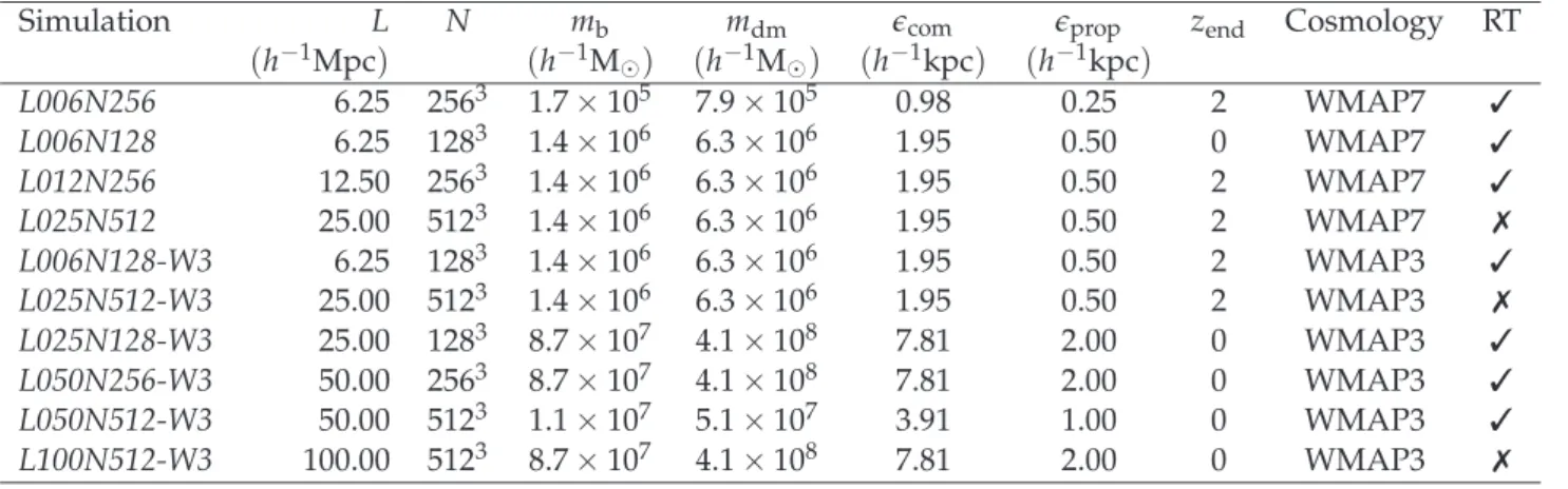
Table 2.1:List of cosmological simulations used in this work. All the simulations use model ingredients identical to the reference simulation
ofSchaye et al.(2010). From left to right the columns show: simulation identifier; comoving box size; number of dark matter particles (there are equally many baryonic particles); initial baryonic particle mass; dark matter particle mass; comoving (Plummer-equivalent) gravitational softening; maximum physical softening; final redshift; cosmology. The last column shows whether the simulation was post-processed with RT. In simulations without RT, the Hidistribution is obtained by using a fit to the photoionization rates as a function of density measured
from simulations with RT.
Simulation L N mb mdm ǫcom ǫprop zend Cosmology RT (h−1Mpc) (h−1M⊙) (h−1M⊙) (h−1kpc) (h−1kpc)
L006N256 6.25 2563 1.7×10⁵ 7.9×10⁵ 0.98 0.25 2 WMAP7 ✓
L006N128 6.25 1283 1.4×10⁶ 6.3×10⁶ 1.95 0.50 0 WMAP7 ✓ L012N256 12.50 2563 1.4×10⁶ 6.3×10⁶ 1.95 0.50 2 WMAP7 ✓ L025N512 25.00 5123 1.4×10⁶ 6.3×10⁶ 1.95 0.50 2 WMAP7 ✗ L006N128-W3 6.25 1283 1.4×10⁶ 6.3×10⁶ 1.95 0.50 2 WMAP3 ✓ L025N512-W3 25.00 5123 1.4×10⁶ 6.3×10⁶ 1.95 0.50 2 WMAP3 ✗ L025N128-W3 25.00 1283 8.7×10⁷ 4.1×10⁸ 7.81 2.00 0 WMAP3 ✓
L050N256-W3 50.00 2563 8.7×10⁷ 4.1×10⁸ 7.81 2.00 0 WMAP3 ✓ L050N512-W3 50.00 5123 1.1×10⁷ 5.1×10⁷ 3.91 1.00 0 WMAP3 ✓ L100N512-W3 100.00 5123 8.7×10⁷ 4.1×10⁸ 7.81 2.00 0 WMAP3 ✗
frequency bins. We setNRC=8 for which our tests yield converged results. Photon packets are transported along their propagation direction until they reach the distance they are allowed to travel within the RT time step by the finite speed of light, i.e.,c∆t. Photon packets that cross the simulation box boundaries
are assumed to be lost from the computational domain. We use a time step
∆t = 1 Myr Lbox 6.25 h−1Mpc
4 1+z
128 NSPH
, whereNSPH is the number of SPH particles in each dimension. We verified that our results are insensitive to the exact value of the RT time step: values that are smaller or larger by a factor of two produce essentially identical results. This is mostly because we evolve the ionization balance on smaller subcycling steps, and because we iterate for the equilibrium solution, as we discuss below. At the end of each time step the ionization states of the particles are updated based on the number of absorbed ionizing photons.
The number of ionizing photons that are absorbed during the propagation of a photon packet from one particle to its neighbor is given by δNabs,ν =
δNin,ν[1−exp(−τ(ν))]whereδNin,νandτ(ν)are, respectively, the initial
num-ber of ionizing photons in the photon packet with frequencyνand the total op-tical depth of all the absorbing species. In this work we mainly consider hydro-gen ionization, but in hydro-general the total optical depth is the sumτ(ν) =∑ατα(ν)
of the optical depth of each absorbing species (i.e.,α∈ {HI, HeI, HeII}). Assum-ing that neighborAssum-ing SPH particles have similar densities, we approximate the optical depth of each species usingτα(ν) =σα(ν)nαdabs, wherenαis the number
density of species,dabsis the absorption distance between the SPH particle and its neighbor andσα(ν)is the absorption cross section (Verner et al.,1996). Note
that ViPs are deleted after each transmission, and hence the photons they absorb need to be distributed among their SPH neighbors. However, in order to de-crease the amount of smoothing associated with this redistribution of photons, ViPs are assigned only 5 (instead of 48) SPH neighbors. We demonstrate conver-gence of our results with the number of ViP neighbors in Appendix C.
At the end of each RT time step, every SPH particle has a total number of ionizing photons that have been absorbed by each species, ∆Nabs,α(ν). This
number is used in order to calculate the photoionization rate of every species for that SPH particle. For instance, the hydrogen photoionization rate is given by:
ΓHI = ∑ν∆Nabs,HI(ν)
ηHINH∆t , (2.1)
where NH is the total number of hydrogen atoms inside the SPH particle and ηHI≡nHI/nH is the hydrogen neutral fraction.
Once the photoionization rate is known, the evolution of the ionization states is calculated. For instance, the equation which governs the ionization state of hydrogen is
dηHI
On the evolution of theHiCDDF
where ne is the free electron number density, Γe,H is the collisional ionization
rate and αHII is the HII recombination rate. The differential equations which govern the ionization balance (e.g., equation2.2) are solved using a subcycling time step, δt = min(fτeq,∆t) where τeq ≡ τionτrec/(τion+τrec), and f is a
di-mensionless factor which controls the integration accuracy (we set it to 10−3), τrec ≡ 1/∑ineαi and τion ≡ 1/∑i(Γi+neΓe,i). The subcycling scheme allows the RT time step to be chosen independently of the photoionization and recom-bination time scales without compromising the accuracy of the ionization state calculations2.
We employ separate frequency bins to transport UVB and RR photons. Be-cause the propagation directions of photons in different frequency bins are merged separately, this allows us to track the individual radiation components, i.e., UVB and RR, and to compute their contributions to the total photoioniza-tion rate. The implementaphotoioniza-tion of the UVB and the recombinaphotoioniza-tion radiaphotoioniza-tion is described in §2.2.3and §2.2.4below.
At the start of the RT, the hydrogen is assumed to be neutral. In ad-dition, we use a common simplification (e.g., Faucher-Giguère et al., 2009; McQuinn & Switzer,2010;Altay et al.,2011) by assuming a hydrogen mass frac-tion of unity, i.e., we ignore helium (only for the RT). To calculate recombinafrac-tion and collisional ionizations rates, we set, in post-processing, the temperatures of star-forming gas particles with densitiesnH >0.1 cm−3toTISM =104K, which
is typical of the observed warm-neutral phase of the ISM. This is needed be-cause in our hydrodynamical simulations the star-forming gas particles follow a polytropic equation of state which defines their effective temperatures. These temperatures are only a measure of the imposed pressure and do not represent physical temperatures (seeSchaye & Dalla Vecchia,2008). To speed up conver-gence, the hydrogen at low densities (i.e.,nH <10−3 cm−3) or high temperatures
(i.e.,T > 105 K) is assumed to be in ionization equilibrium with the UVB and
the collisional ionization rate (see Appendix A2). Typically, the neutral fraction of the box and the resulting HiCDDF do not evolve after 2-3 light-crossing times
(the light-crossing time for the extended box withLbox=6.25 comovingh−1Mpc is≈7.5 Myr at z = 3).
2.2.3
Ionizing background radiation
Although our hydrodynamical simulations are performed using periodic bound-ary conditions, we use absorbing boundbound-ary conditions for the RT. This is neces-sary because our box size is much smaller than the mean free path of ionizing photons. We simulate the ionizing background radiation as plane-parallel
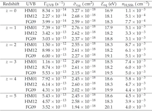
Table 2.2: Hydrogen photoionization rate, absorption cross-section, equivalent gray ap-proximation frequency and the self-shielding density threshold (i.e., based on equa-tion 2.13) for three UVB models: Haardt & Madau (2001) (HM01; used in this work), Haardt & Madau(2012) (HM12) andFaucher-Giguère et al.(2009) (FG09) at different red-shifts. For the calculation of the photoionization rate and absorption cross-sections, only photons with energies below 54.4 eV are taken into account, effectively assuming that more energetic photons are absorbed by He.
Redshift UVB ΓUVB(s−1) σ¯νHI ( cm2) Eeq(eV) nH,SSh( cm−3)
On the evolution of theHiCDDF
ation entering the simulation box from its sides. At the beginning of each RT step, we generate a large number of photon packets,Nbg, on the nodes of a reg-ular grid at each side of the simulation box and set their propagation directions perpendicular to the sides. The number of photon packets is chosen to obtain converged results. Furthermore, to avoid numerical artifacts close to the edges of the box, we use the periodicity of our simulations to extend the simulation box by the typical size of the region where we generate the background radiation (i.e., 2% of the box size from each side). These extended regions are excluded from the analysis, thereby removing the artifacts without losing any information contained in the original simulation box.
The photon content of each packet is normalized such that in the absence of any absorption (i.e., assuming the optically thin limit), the total photon density of the box corresponds to the desired uniform hydrogen photoionization rate. If we assume that all the photons with frequencies higher thanνHeIIare absorbed by helium, then the hydrogen photoionization rate can be written as:
ΓUVB =
Z νHeII
νHI
4π Jν
hν σHI, ˚ dν
≡ 4πσ¯νHI h
Z νHeII
νHI Jν
ν dν, (2.3)
where Jν is the radiation intensity (in units erg cm−2s−1sr−1Hz−1), νHI and νHeII are respectively the frequency at the Lyman-limit and the frequency at the HeII ionization edge, andσHI, ˚ is the neutral hydrogen absorption cross-section for ionizing photons. In the last equation we have defined the gray absorption cross-section,
¯ σνHI ≡
RνHeII
νHI Jν/ν σHI, ˚ dν
RνHeII
νHI Jν/νdν
. (2.4)
The radiation intensity is related to the photon energy density,uν,
Jν= uνc
4π =
nνhνc
4π , (2.5)
wherenνis the number density of photons inside the box. Combining Equations 2.3-2.5yields
ΓUVB=nνHI cσ¯νHI, (2.6)
wherenνHI is the number density of ionizing photons inside the box. The total number of ionizing photons in the box is therefore given by
nνHIL3box =nγ6 NbgLcbox∆t, (2.7)
wherenγis the number of ionizing photons carried by each photon packet. Now
box during each step in order to achieve the desired Hiphotoionization rate:
nγ=
ΓUVBL2
box ∆t
6 ¯σνHI Nbg , (2.8)
We use the redshift-dependent UVB spectrum ofHaardt & Madau(2001) to calculateΓUVB and ¯σνHI. TheHaardt & Madau (2001) UVB model successfully
reproduces the relative strengths of the observed metal absorption lines in the intergalactic medium (Aguirre et al.,2008) and has been used to calculate heat-ing/cooling in our cosmological simulations 3. We note however that using more recent models for the UVB is not expected to change our main results. On can show that varying the UVB photoionization rate by a factor of 3, only changes the HI CDDF by less than 0.2 dex for LLSs (e.g.,Altay et al.,2011). As shown in Table 2.2, the differences between photoionization rates in different UVB models are smaller that a factor of 3, particularly atz>1, where the
pho-toionization by the UVB is not subdominant (see §2.3.5). The variations in the adopted UVB model is even less important for systems with higher HI column densities (i.e., DLAs) which remain highly neutral for reasonable UVB models (e.g.,Haardt & Madau,2012;Faucher-Giguère et al.,2009).
To reduce the computational cost, we treat the multi-frequency problem in the gray approximation. In other words, we transport the UVB radiation using a single frequency bin, inside which photons are absorbed using the gray cross-section ¯σνHI defined in equation 2.4. Note that the gray approximation ignores the spectral hardening of the radiation field that would occur in multifrequency simulations. In Appendix D we show the result of repeating our simulations us-ing multiple frequency bins, and also explicitly accountus-ing for the absorption of photons by helium. These results clearly show the expected spectral hardening. The impact of spectral hardening on the hydrogen neutral fractions and the Hi
CDDF is small. However, we note that spectral hardening can change the tem-perature of the gas in self-shielded regions and that this effect is not captured in our simulations.
Hydrogen photoionization rates and average absorption cross-sections for UVB radiation at different redshifts are listed in Table2.2for our fiducial UVB model based onHaardt & Madau(2001) together with Haardt & Madau(2012) andFaucher-Giguère et al. (2009). The photoionization rate peaks atz≈ 2−3 in those models and the equivalent effective photon energy4of the background radiation changes only weakly with redshift, compared to the total photoioniza-tion rate.
3Note that during the hydrodynamical simulations, photoheating from the UVB is applied to all gas particles. This ignores the self-shielding of hydrogen atoms against the UVB that occurs at densitiesnH &10−3−10−2cm3. This inconsistency, which could affect both collisional ionization rates and the small-scale structure of the absorbers, has been found to have no significant impact on the simulated HiCDDF (Pontzen et al.,2008;McQuinn & Switzer,2010;Altay et al.,2011).
On the evolution of theHiCDDF
2.2.4
Recombination radiation
Photons produced by the recombination of positive ions and electrons can also ionize the gas. If the recombining gas is optically thin, recombination radiation can escape and its ionizing effects can be ignored (i.e., the so-called Case A). However, for regions in which the gas is optically thick, the proper approxima-tion is to assume the ionizing recombinaapproxima-tion radiaapproxima-tion is absorbed on the spot. In this case, the effective recombination rate can be approximated by exclud-ing the transitions that produce ionizexclud-ing photons (e.g., Osterbrock & Ferland, 2006). This scenario is usually called Case B. A possible way to take into ac-count the effect of recombination radiation is to use Case A recombination at low densities and Case B recombination at high densities (e.g.,Altay et al.,2011; McQuinn et al.,2011), but this will be inaccurate in the transition regime.
In this work we explicitly treat the ionizing photons emitted by recombining hydrogen atoms and follow their propagation through the simulation box. This is facilitated by the fact that the computational cost of RT with TRAPHIC is independent of the number of sources. This is particularly important noting that every SPH particle is potentially a source. The photon production rates of SPH particles depend on their recombination rates and the radiation is emitted isotropically once at the beginning of every RT time step (see Raicevic et al. in prep. for full details).
We do not take into account the redshifting of the recombination photons by peculiar velocities of the emitters, or the Hubble flow. Instead, we assume that all recombination photons are monochromatic with energy 13.6 eV. In real-ity, recombination photons cannot travel to large cosmological distances without being redshifted to frequencies below the Lyman edge. Therefore, neglecting the cosmological redshifting of RR will result in overestimation of its photoioniza-tion rate on large scales. However, because of the small size of our simulaphotoioniza-tion box, the total photoionization rate that is produced by RR on these scales re-mains negligible compared to the UVB photoionization rate. Consequently, the neglect of RR redshifting is not expected to affect our results.
2.2.5
The
H
i
column density distribution function
In order to compare the simulation results with observations, we compute the CDDF of neutral hydrogen, f(NHI,z), a quantity that is somewhat straightfor-ward to measure in QSO absorption line studies and is defined as the number of absorbers per unit column density, per unit absorption length,dX:
f(NHI,z)≡ d 2n
dNHIdX ≡ d2n dNHIdz
H(z) H0
1