Nat. Hazards Earth Syst. Sci., 13, 2089–2099, 2013 www.nat-hazards-earth-syst-sci.net/13/2089/2013/ doi:10.5194/nhess-13-2089-2013
© Author(s) 2013. CC Attribution 3.0 License.
EGU Journal Logos (RGB)
Advances in
Geosciences
Open Access
Natural Hazards
and Earth System
Sciences
Open Access
Annales
Geophysicae
Open Access
Nonlinear Processes
in Geophysics
Open Access
Atmospheric
Chemistry
and Physics
Open Access
Atmospheric
Chemistry
and Physics
Open Access
Discussions
Atmospheric
Measurement
Techniques
Open Access
Atmospheric
Measurement
Techniques
Open Access
Discussions
Biogeosciences
Open Access Open Access
Biogeosciences
Discussions
Climate
of the Past
Open Access Open Access
Climate
of the Past
Discussions
Earth System
Dynamics
Open Access Open Access
Earth System
Dynamics
Discussions
Geoscientific
Instrumentation
Methods and
Data Systems
Open Access
Geoscientific
Instrumentation
Methods and
Data Systems
Open Access
Discussions
Geoscientific
Model Development
Open Access Open Access
Geoscientific
Model Development
DiscussionsHydrology and
Earth System
Sciences
Open Access
Hydrology and
Earth System
Sciences
Open Access
Discussions
Ocean Science
Open Access Open Access
Ocean Science
Discussions
Solid Earth
Open Access Open Access
Solid Earth
Discussions
Open Access Open Access
The Cryosphere
Natural Hazards
and Earth System
Sciences
Open Access
Discussions
Evaluation and projection of daily temperature percentiles from
statistical and dynamical downscaling methods
A. Casanueva1, S. Herrera1,2, J. Fern´andez1, M. D. Fr´ıas1, and J. M. Guti´errez3
1Grupo de Meteorolog´ıa, Dpto. Matem´atica Aplicada y Ciencias de la Computaci´on, Univ. de Cantabria,
Avda. de los Castros, s/n, 39005 Santander, Spain
2Predictia Intelligent Data Solutions, S.L. CDTUC, Avda. de los Castros, s/n, 39005, Santander, Spain 3Grupo de Meteorolog´ıa, Instituto de F´ısica de Cantabria, CSIC-Univ. de Cantabria, Avda. de los Castros, s/n,
39005 Santander, Spain
Correspondence to: A. Casanueva ([email protected])
Received: 26 November 2012 – Published in Nat. Hazards Earth Syst. Sci. Discuss.: – Revised: 29 April 2013 – Accepted: 31 May 2013 – Published: 22 August 2013
Abstract. The study of extreme events has become of great
interest in recent years due to their direct impact on soci-ety. Extremes are usually evaluated by using extreme indi-cators, based on order statistics on the tail of the probability distribution function (typically percentiles). In this study, we focus on the tail of the distribution of daily maximum and minimum temperatures. For this purpose, we analyse high (95th) and low (5th) percentiles in daily maximum and min-imum temperatures on the Iberian Peninsula, respectively, derived from different downscaling methods (statistical and dynamical). First, we analyse the performance of reanalysis-driven downscaling methods in present climate conditions. The comparison among the different methods is performed in terms of the bias of seasonal percentiles, considering as ob-servations the public gridded data sets E-OBS and Spain02, and obtaining an estimation of both the mean and spatial percentile errors. Secondly, we analyse the increments of fu-ture percentile projections under the SRES A1B scenario and compare them with those corresponding to the mean tempe-rature, showing that their relative importance depends on the method, and stressing the need to consider an ensemble of methodologies.
1 Introduction
Extreme temperature events have increased over most re-gions of the globe in the last decades (Alexander et al., 2006). Their analysis can be approached by means of extreme value
indices or by extreme value distributions. Extreme value in-dices are the most commonly used approach for this problem and characterize extremes using percentiles and/or frequen-cies of days exceeding certain thresholds. The Expert Team on Climate Change Detection and Indices (ETCCDI; Tank et al., 2009) defined a standard set of these indices, which are now widespread in the literature and enable the com-parison of the results obtained in different studies. Some of these indices are based on the computation of high or low percentiles as reference, linking the lowest minimum peratures to frost hazard risk and the highest maximum tem-peratures to heat stress conditions. In this study, we focus directly on extreme percentiles and their representation and future projection according to an ensemble of state-of-the-art regional climate downscaling techniques.
Climate downscaling techniques bridge the gap between the large scale circulation simulated by global climate mod-els (GCMs) and the climate information at regional scale, which is modulated by local features (orography, coast-lines, vegetation distribution, etc.) not resolved by the GCMs (Giorgi and Mearns, 1991). In the early 1990s, the two most common downscaling approaches were introduced: sta-tistical and dynamical. Stasta-tistical downscaling (SD) con-sists in building empirical models relating large-scale vari-ables, which are well represented by GCMs, with local ob-servations. The empirical model is then applied to future large-scale fields simulated by GCMs. Dynamical downscal-ing (DD) is commonly implemented as a regional climate model (RCM), which solves the governing equations of the
atmosphere at a higher resolution over a limited spatial do-main, using the coarse GCM fields as boundary conditions.
One of the main limitations of SD methods is that they might suffer from non-stationarity problems (i.e. being un-able to represent altered climates other than that used during the training period). RCMs are expected to respond realisti-cally to the forcings and develop altered climates if required. However, they might also suffer from non-stationarity prob-lems due to the use of parameterizations to represent the ef-fect of the smaller-scale processes. Some recent studies in-dicate that non-stationarity might not be a major issue for some SD methodologies for mean values (Fr´ıas et al., 2006; Guti´errez et al., 2013), but the influence of this problem in the extremes is still an open issue, in particular regarding the extreme percentiles of the downscaled series.
The comparative studies of SD and DD reported in the li-terature (Kidson and Thompson, 1998; Mearns et al., 1999; Murphy, 1999, 2000; Hellstrom et al., 2001; Haylock et al., 2006; Schmidli et al., 2007) demonstrated that both down-scaling approaches have comparable skill in representing re-gional climates, with the best-performing methods depend-ing on the particular variables, season and region analysed.
With regard to the performance of the downscaling me-thods for reproducing extreme percentiles, Kjellstr¨om et al. (2007) studied the RCM bias in maximum and minimum temperature percentiles against station data and obtained that the models generally overestimate maximum temperatures in southern Europe during summer. The RCMs in this study were not driven by reanalysis data, and thus the biases could arise from the driving GCM. They also found that the bi-ases generally increase towards the tails of the probability distributions and they reduce significantly when the ensem-ble average is considered. In a more recent work Kjellstr¨om et al. (2010) evaluate the ENSEMBLES RCM database, ar-riving at similar conclusions. On the other hand, Hertig et al. (2010) assessed the performance of regression-based statis-tical downscaling techniques to reproduce extreme tempe-rature percentiles in the Mediterranean using different sets of predictors. They conclude that, despite the similar perfor-mance of the large-scale predictors in reproducing extreme indicators in present climate, the downscaling of future pro-jections vary considerably depending on the particular pre-dictors used. They emphasize that changes in temperature ex-tremes do not follow a simple shift of the whole distribution to increased values.
However, as far as we know, there is no comparison study on the relative benefits of each of those techniques in or-der to reproduce extreme temperature percentiles. In this work we analyse this problem considering a state-of-the-art ensemble of dynamical and statistical downscaled data in present climate conditions and future projections. The EU-funded ENSEMBLES project (2005–2009; van der Linden and Mitchell, 2009) has produced the largest database of RCM simulations over Europe to date. Despite that SD was also pursued in the project, to our knowledge there has not
been any systematic comparison of the SD and RCM results. The recently finished ESTCENA project (http://www.meteo. unican.es/projects/estcena), funded by the Spanish R&D pro-gramme, provides an opportunity for such a comparison over Spain since several SD techniques developed within the EN-SEMBLES project were trained with the same reanalysis (ERA-40) used in the evaluation runs of the ENSEMBLES RCMs and applied to the same GCMs which provided the boundary conditions in that project.
Finally, when evaluating extremes, it is of great impor-tance to take into account the errors introduced by the ob-servations used as reference. For instance, some studies us-ing the state-of-the-art gridded observational data set for Eu-rope (E-OBS, Haylock et al., 2008; Hofstra et al., 2009) as reference data set to evaluate RCM results have reported that large model biases are found in regions with low sta-tion density (Garc´ıa-D´ıez et al., 2013; Kjellstr¨om et al., 2010; Nikulin et al., 2011). Note that this problem is critical for ex-tremes since the actual exex-tremes could be underestimated in the gridded observational data due to the interpolation pro-cess (see, e.g. Hofstra et al., 2010; Lenderink, 2010). To test the sensitivity of the results to the observational data set, we compare the simulated extremes at regional scale against two different data sets: E-OBS and Spain02 (Herrera, 2011; Herrera et al., 2012).
This work is organized as follows. In Sect. 2 we present the data used in this study. Section 3 presents the methodol-ogy followed to assess the performance of the downscaling methods with respect to extreme percentiles. The results are given in Sect. 4. Finally, the conclusions of this work are given in Sect. 5.
2 Data
Two high-resolution gridded data sets (E-OBS and Spain02) have been considered as reference observations to compare the downscaled results.
The E-OBS data set is the state-of-the-art daily freely available high-resolution gridded observational data set for Europe (Haylock et al., 2008; Hofstra et al., 2009). This data set has been developed within the EU-funded ENSEM-BLES Project (http://www.ensembles-eu.org) and provides daily values of mean, maximum and minimum temperatures and accumulated precipitation for the period 1950–2010 (in version 5.0, used in this study). It has been obtained by the interpolation of more than 2300 observational stations over Europe. It presents advantages with respect to previous prod-ucts considering higher spatial resolution and coverage, pe-riod of study and number of stations. In particular, version 5.0 increases the number of stations in Spain and Germany with respect to the previous one.
minimum temperature data set covering continental Spain and the Balearic Islands with 0.2◦resolution. The
interpola-tion of temperature follows the same procedure as in E-OBS, but the product is based on a larger number of surface sta-tions (thousands of stasta-tions) which have been selected using a stringent quality control to cover the whole period (1950– 2008) with few missing data. This data set is able to repro-duce the intensity and spatial variability of the typical ob-served extremes. Although extremes are more sensitive to interpolation, the dense station coverage was crucial to get an accurate reproduction of these events.
The SD data used in this study was generated within the ESTCENA project (2008–2011), which aimed at generat-ing regional climate change scenarios over Spain usgenerat-ing SD methods (Guti´errez et al., 2013). In particular, five SD me-thods were applied in this project: a non-linear analogue method considering the Euclidean distance to obtain a sin-gle nearest neighbour (S1, hereafter), three multiple linear regression methods, the first one considering the principal components (PCs) of the predictors explaining 95 % of their variance up to a maximum of 30 PCs (S2), another method considering 15 PCs plus the nearest gridbox values (S3), the third one a combination of weather types (WTs) by k-means and the S3 method (S4) and, finally, a pure weather-typing method (100 WTs) combined with a Gaussian weather gen-erator for each WT (S5). These five methods cover the sta-tistical methodologies with the best results for the Iberian Peninsula according to Guti´errez et al. (2013). Bear in mind that S2, S3 and S4 are connected since they are based on multiple regression models. Table 1 summarizes these me-thods and the variables considered as predictors in the down-scaling. In most of the experiments, sea level pressure (SLP) and daily mean temperature (T2m) were selected as predic-tors. The SD models were trained in perfect prog condi-tions using the 40 yr reanalysis from the European Centre for Medium Range Weather Forecasts (ERA-40; Uppala et al., 2005) as large-scale predictor for the Spain02 surface pre-dictands. The calibrated SD models were then applied to two GCMs, ECHAM5 and HADCM3Q0, considering the SRES A1B scenario.
The RCM data used in this study were generated in the ENSEMBLES project. This project was a collaborative ef-fort of different European meteorological institutions, and it focused on the generation of climate change scenarios over Europe. ENSEMBLES studied the climate change in Europe from different perspectives and considering different spatial and temporal scales. In particular, dynamical downscaling of GCM simulations was performed using nine different RCMs run by different institutions over a common area covering the entire continental European region with a common reso-lution of 25 km. Within ENSEMBLES, an initial RCM eval-uation experiment was carried out using the ERA-40 reanal-ysis as “perfect” boundary conditions. All RCM evaluation runs cover the common period 1961–2000 (although some of them simulated longer periods). In this study we focus on
the simulations from the five RCMs shown in Table 2, here-after labelled as D1–D5, which performed best in a previ-ous analysis over this area (Herrera et al., 2010). The GCM boundary conditions (ECHAM5 or HADCM3Q0) and sce-nario (A1B) are exactly those considered in the SD models, thus enabling a systematic comparison of the statistical and dynamical approaches.
3 Methodology
Our analysis for the evaluation of the different downscaling models focuses on the biases of the maximum and minimum temperature percentiles (5th percentile of minimum tempe-rature and 95th percentile of maximum tempetempe-rature) in the period 1971–2000. This 30 yr period is common to all ob-servational databases used in all downscaling estimates. The same period is used as present-climate reference for the com-putation of “delta” changes (R¨ais¨anen, 2007), which is also considered in order to compare the different estimates under a future climate change scenario. We considered near (2021– 2050) and far (2070–2099) future periods. Notice that the driving GCMs in all future projections considered are forced by the SRES A1B emissions scenario.
The performance of the different downscaling methods varies seasonally (see, e.g. Fowler and Ekstrom, 2009). Therefore, we considered separately the biases and deltas in winter (DJF) and summer (JJA). For the bias computations, the downscaling estimates were interpolated to the corre-sponding observational grid by means of a nearest neighbour approach. This preserves the extreme values better than, for instance, bilinear interpolation, which smoothes the extremes by averaging them with nearby values.
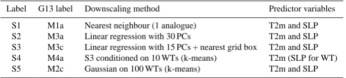
Table 1. Statistical downscaling methods and predictors. The second column is the label in Guti´errez et al. (2013), which provides further details of the different methods.
Label G13 label Downscaling method Predictor variables
S1 M1a Nearest neighbour (1 analogue) T2m and SLP S2 M3a Linear regression with 30 PCs T2m and SLP S3 M3c Linear regression with 15 PCs + nearest grid box T2m and SLP S4 M4a S3 conditioned on 10 WTs (k-means) T2m (SLP for WT) S5 M2c Gaussian on 100 WTs (k-means) T2m and SLP
Table 2. Summary of the ENSEMBLES RCM simulations used in the study.
Label RCM GCM Institution Reference
D1 CLM HADCM3Q0 Swiss Institute of Technology Jaeger et al. (2008) D2 HadRM3 Q0 HADCM3Q0 Hadley Centre/UK Met Office Collins et al. (2006) D3 RACMO ECHAM5 Koninklijk Nederlands Meteorologisch Instituut van Meijgaard et al. (2008) D4 M-REMO ECHAM5 Max Planck Institute for Meteorology Jacob et al. (2001) D5 PROMES HADCM3Q0 Universidad de Castilla la Mancha S´anchez et al. (2004)
information about the kind of defects that these methods present and which part of the errors in the extreme percentiles can be ascribed to biases in the mean and/or the standard de-viation. The correction of these two moments of the probabil-ity densprobabil-ity function (PDF) also happen to be the simplest and most widely used bias correction methods. Our work does not aim to introduce any improvement to the existing bias correction literature, which is currently pursuing the correc-tion of more sophisticated bias features, such as temperature-dependent biases (see, e.g. Christensen and Boberg, 2012).
The correction of the mean of the distribution was com-puted as
xim0=xim−xs(i)m +xs(i)o , (1) wherexiis the value of a daily variable at timei. Superscripts
o and m refer to observed and model values, respectively, and
s(i)is the season corresponding to dayi.
If the correction of the bias in the mean of the distribution does not improve the bias in a percentile, that could imply that the variability is wrongly represented. Thus, after cor-recting the mean, a second-order bias correction can be done considering the standard deviation (σ). This correction was computed as
xim00=
xim−xs(i)m σ o
s(i)
σs(i)m +x o
s(i), (2)
whereσ is the standard deviation for each seasons(i) corre-sponding to dayi.
A final correction was applied to the RCMs to account for the difference in altitude between the RCM grid point and the observational record (Chadwick et al., 2011). The correction was simply computed by means of a constant lapse rate of
6.5 K km−1:
ximh=xim−0.0065· ho−hm
, (3)
wherehis the corresponding height in metres. This bias cor-rection is not necessary in the statistical methods, since pre-dictions are done in the points where observational data are collected. For RCMs, our results were not significantly af-fected by this correction (not shown), which is very small in most places. Therefore, the sensitivity of the results to this correction is not shown in the following.
Bias corrections in Eqs. (1) and (2) were only applied in the present climate evaluation. However, in the future climate analysis no information about the observations was trans-ferred to the models.
4 Results
percentile 90 percentile 95
Maximum Temperature
percentile 5 percentile 10
DJF
JJA
Minimum Temperature
12 14 16 18 20
30 32 34 36 38
−4 −2 0 2
6 8 10 12 14
(ºC) (ºC)
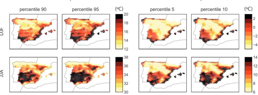
Fig. 1. Observed percentiles for maximum (90th and 95th) and minimum (5th and 10th) temperature in winter and summer according to the Spain02 data set.
that they sample the tails of the probability distribution. How-ever, they are not associated with rare events, since their val-ues are reached on average once every 20 days (i.e. more than 4 days per season). Note also that higher percentiles (e.g. 99th) would lead to unreliable estimates due to the small sample size.
4.1 Evaluation in present climate conditions
The downscaling methods are first evaluated in present cli-mate conditions, using reanalysis-driven simulations in the period 1971–2000. To this end, downscaled values from ERA-40 reanalysis (considered as “perfect” GCM output; Brands et al., 2012) are compared to the two reference ob-served data sets, Spain02 and E-OBS. Figure 2 shows the spatially averaged biases in summer (JJA) and winter (DJF) for the 5th (upper panels) and 95th (lower panels) percentiles using Spain02 (left) and E-OBS (right) reference data sets. This figure allows comparing the biases of both statistical and dynamical downscaling values, considering both the original and the unbiased downscaled values. Each line in this plot corresponds to a downscaling method: in black for dynamical downscaling and in red for statistical downscaling techniques (see the caption for details). For example, the rightmost line in Fig. 2a corresponds to the dynamical (black line) down-scaling method 4 (according to the label), i.e. D4 or REMO model, and shows an averaged bias in the 5th percentile of minimum temperature with respect to Spain02 (this is the bias shown in all lines in this panel) of about +3.5◦C in
win-ter and +2◦C in summer. After the correction of the seasonal
mean bias, the labelled end of the line shows the remaining bias in the 5th percentile: +1.5◦C in winter and –0.4◦C in summer. These biases are due to deviations in higher-order moments of the PDF. Finally, the spatial variability of the bias pattern in REMO is larger in winter than in summer (the horizontal section of the cross is longer than the vertical sec-tion). This spatial variability is reduced when the seasonal
mean correction is applied (the cross at the origin is larger than the cross at the labelled end of the line).
When considering the original data (unlabelled crosses), it is shown that the dynamical methods (black) show larger bi-ases than the statistical ones (red), in particular for the 95th percentile. For the dynamical approach, after bias correction (crosses labelled with numbers), the resulting percentile bi-ases become smaller, moving in general towards the origin (zero bias). This pattern is found with both reference data sets (Spain02 and E-OBS) for both summer and winter. The spa-tial dispersion (given by the length of the crosses) is similar for both Spain02 and E-OBS, being larger in winter than in summer for the 5th percentile, whereas the opposite is found for the 95th percentile. In both cases, the differences are re-duced with the correction in the seasonal mean.
For the statistical approaches (red crosses) both the mean biases and the spatial variability are larger in the E-OBS case, thus indicating that spatial variability is clearly affected by the baseline climate data set used to fit/compare the empirical models. Biases found for the statistical methods are smaller than for the dynamical ones and they do change only slightly with the bias correction (except for 95th percentile). Statisti-cal methods seem to be separated into two clusters: one com-posed of methods based on linear regressions S2–4, and a second cluster composed of S1 based on analogues and S5 based on a combination of a Gaussian weather generator with the k-means weather typing. Moreover, for methods S2–4 the bias correction in the mean leads to larger biases in the per-centiles, e.g. for the 95th percentile in winter. This indicates a good result for the wrong reason, probably caused by an er-ror cancellation between the mean and the variability of the statistically downscaled data using these methods.
−4 −3 −2 −1 0 1 2 3 4
−4
−3
−2
−1 0 1 2 3 4
R R
R R
12 34
5 1 2 3
4 5
bias 5p DJF
bias 5p JJA
E
−4 −3 −2 −1 0 1 2 3 4
−4
−3
−2
−1
0 1 2 3 4
1 234
5 1 2 3
4 5
bias 5p DJF
bias 5p JJA
−4 −3 −2 −1 0 1 2 3 4
−4
−3
−2
−1
0 1 2 3 4
1
23 4
5 1 2
3 4
5
bias 95p DJF
bias 95p JJA
−4 −3 −2 −1 0 1 2 3 4
−4
−3
−2
−1 0 1 2 3 4
1
23 4
5 12 3
45
bias 95p DJF
bias 95p JJA
σref=3ºC σref=3ºC
σref=3ºC σref=3ºC
E
(a)
S B O -E . f e R 2
0 n i a p S . f e R
(b)
(c) (d)
Fig. 2. Spatially averaged bias (in◦C) of 5th percentile of daily minimum (upper panels) and 95th percentile of daily maximum (lower panels) temperature with respect to Spain02 (left panels) and E-OBS (right panels). Each panel is a Cartesian (scatter) plot of the summer (JJA,yaxis) bias against the winter (DJF,xaxis) one. The origin (the unlabelled end) of a line represents the seasonal biases in the percentile when no correction is applied. The end of each line (the labelled end) represents the biases when the seasonal mean bias is corrected (Eq. 1). The line of each method is labelled according to Tables 1 and 2; note that the “D” (“S”) initial letters have been dropped for visual clarity. RCM (SD) lines are depicted in black (red). The lines corresponding to the reanalysis (blue) and to E-OBS (pink) are also depicted for reference. Finally, crosses at each end represent the spatial standard deviation of the biases. For clarity,σ values are rescaled; the value
σref=3◦C is shown as reference.
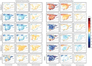
pink line in Fig. 2a and c shows the biases (mean differences) from E-OBS with respect to Spain02. In the case of the 95th percentile the average difference over the Iberian Peninsula is 0.5◦C, whereas it is negligible for the 5th percentile. These differences vanish when considering the bias-corrected data. In order to better assess the spatial structure of percentile biases, Figs. 3 and 4 represent the spatial bias of the 5th and 95th percentiles in winter and summer for minimum and maximum temperatures, respectively. In each figure, the first five rows show the percentile biases for the five statistical (left panel) and the five dynamical (right panel) methods with respect to Spain02, whereas the last row corresponds to the biases of E-OBS (left panel) and ERA-40 (right panel) with respect to Spain02. The first column of each panel represents the corresponding bias without doing any correction; the sec-ond and third columns represent the biases when the first-(mean) and, additionally, second- (standard deviation) order corrections are applied to the predictions. Maps for the five statistical methods exhibit a negligible bias decrease when
the correction in the mean is applied (second column). As pointed out above, similar warm/cold bias patterns are ob-served for S2–4 for the 5th and 95th percentiles, respectively. On the other hand, the S5 method presents a slight cold/warm bias pattern and the S1 method a small spatially changing bias pattern. For all these methods the bias at all grid points is below 0.5◦C when the second-order correction is applied.
Statistical Downscaling
Uncorrected Mean Correction Uncorrected
Dynamical Downscaling
M
ethod 1
M
ethod 2
M
ethod 3
M
ethod 4
M
ethod 5
(ºC)
−5 −4 −3 −2 −1 0 1 2 3 4 5
Std Correction
EOBS
Mean Correction Std Correction
ER
A40
Fig. 3. Spatial bias distribution (in◦C) for the 5th percentile of daily minimum temperature for statistical (left panel) and dynamical (right panel) methods with respect to Spain02 in winter. The first column of each panel represent the bias without doing any correction. The second column represents the bias when the correction in the seasonal mean is done. The third column represents the bias when the second-order correction is done. E-OBS and ERA-40 biases with respect Spain02 are also included in the last row.
Statistical Downscaling
Uncorrected Mean Correction Uncorrected
Dynamical Downscaling
M
ethod 1
M
ethod 2
M
ethod 3
M
ethod 4
M
ethod 5
(ºC)
−5 −4 −3 −2 −1
0
1 2 3 4 5
Std Correction
EOBS
Mean Correction Std Correction
ER
A40
percentile are remarkable. D1 and D2 show a strong warm bias, whereas D3–5 show a cold bias. In all cases, the RCMs tend to be warmer over coastal areas. This warm/cold be-haviour is kept, with lower intensity, even after the first-order correction. Only after the variability correction do the RCMs reduce their biases.
The spatial distribution of the differences between E-OBS and Spain02 is also shown in Figs. 3 and 4 (last row, left panel), exhibiting large differences when no correction is applied (up to 3–4◦C). Differences in the mean values of a similar magnitude have also been reported by G´omez-Navarro et al. (2012). The bias is largely reduced with the first-order correction in both cases, with an additional reduc-tion with the standard deviareduc-tion correcreduc-tion for the 5th per-centile. Results for ERA40 (right panels, last row) present positive/negative biases higher than 4◦C in magnitude in a
huge part of the Iberian Peninsula for 5th/95th percentiles. For maximum temperature (95th percentile), the bias pattern is clearly related to the orography, unlike the continentality-driven pattern found in the RCMs.
4.2 Mean and percentile changes in future climate
In this section we apply the standard “delta method” to anal-yse the climate change signal for extreme percentiles and also to analyse the level of uncertainty according to the re-sults of the previous section. To this aim, the difference of the 21st century (A1B emission scenario) and control (20C3M) downscaled simulations is computed considering two future periods (2021–2050 and 2070–2099) and the same control one (1971–2000), and two different GCMs: ECHAM5 and HADCMQ0. Moreover, the increments obtained for the 95th and 5th percentiles are here compared with those correspond-ing to the mean values, in winter and summer, for each down-scaling method. The idea is to assess whether the climate change signal is higher for the extremes than for the mean values.
Figures 5 and 6 show the spatially averaged delta values (and the spatial variability, represented by the crosses) over the Iberian Peninsula for the two periods considered, respec-tively. Colours of lines and labels are the same as in the previous cases. However, now, the labelled end shows the delta values for the percentiles, whereas the unlabelled end indicates the delta for the mean values. The crosses repre-sent the standard deviation of the increments over the Iberian Peninsula, which has been rescaled between 0 and 1◦C, as
shown in the figures. Results for the 5th percentile for mini-mum temperature are shown in the left panels of the figures and results for the 95th percentile for maximum temperature are shown in the right panel; in all cases winter values are represented in thex axis and summer values in the y axis. Values from the statistical downscaling methods are plotted in red (light red for those using ECHAM5 GCM and dark red for those considering the HADCM3Q0) and from the dynamical downscaling in grey (light grey for those nested
into ECHAM5 and dark grey — black – for those nested in HADCM3Q0).
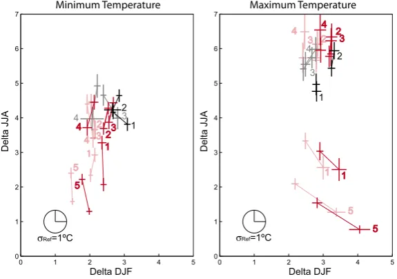
The resulting values for both periods (Figs. 5 and 6) show an increase in both the mean and percentile values (note that the axes only show positive values), with higher values in the second period for both the mean and the percentiles, in agreement with Fischer and Sch¨ar (2010). However, there is no consistent indication that the change in percentiles is higher than changes in the mean; this varies from case to case, depending on the GCM or the downscaling approach. In general, increments are higher in summer than in winter for both percentiles. The increases for minimum temperatures in winter show more consistency among the different methods compared to the changes for maximum temperatures in sum-mer. This result is in agreement with Hertig et al. (2010). The most remarkable result is the anomalous behaviour obtained for the statistical downscaling methods 1 and 5 (analogues and weather-typing methods, see Table 1) for maximum tem-perature in summer. In this case, the methods are clear out-liers with respect to the rest of methodologies – particularly in the final period 2070–2099; see Fig. 6, where the problem also affects the minimum temperature – due to a large under-estimation of both the mean and percentile values, more pro-nounced in the latter case. This result is in agreement with Guti´errez et al. (2013), where these two methods were re-ported to be non-robust in climate change conditions, parti-cularly for maximum temperature in summer, since they have no extrapolation capabilities. Our results show that this prob-lem is even more pronounced for high/low percentiles. Apart from this anomalous behaviour, the results for the different GCM and downscaling method combinations for the near fu-ture period (2021–2050) cluster first according to the parti-cular election of GCM, and then by the downscaling family (either statistical or dynamical), being that the variability of the different statistical (or dynamical) downscaling methods is the smallest source of uncertainty. However, this does not hold by the end of the century (2070–2099), when the contri-bution to the total variability is shared similarly by all factors. Both in the near (Fig. 5) and far (Fig. 6) future periods, the differences between the percentiles and the mean tempe-rature values are, in general, higher in summer than in winter and thus also the spatial variability of the results. Finally, the spatial variability of the climate change signal (the delta) for the percentiles is of the same order of the error committed when reproducing percentiles in perfect conditions, consi-dering the case where the mean is corrected (note that the delta method does implicitly perform an approximate can-cellation of the mean).
5 Conclusions
0 0.5 1 1.5 2 2.5 3 0
0.5 1 1.5 2 2.5 3 3.5 4 4.5 5
1 2
3 4
5
34 1
2 3 4
5
1 2
5
Delta DJF
Delta JJA
Maximum Temperature
0 0.5 1 1.5 2 2.5 3
0 0.5 1 1.5 2 2.5 3 3.5 4 4.5 5
1 2 3 4 5
3 4
1 23 4
5 1
2
5
Delta DJF
Delta JJA
σRef=1ºC
Minimum Temperature
σRef=1ºC
Fig. 5. Delta values (in◦C) averaged over the Iberian Peninsula for the period 2021–2050 of A1B scenario with respect to 1971–2000 of 20C3M. The origin (the unlabelled end) of a line represents delta values calculated for the mean values of minimum (left) and maximum (right) temperature in winter (DJF,xaxis) and summer (JJA,yaxis). The end of the line (the labelled end) is the delta value for the 5th percentile (left) and the 95th percentile (right) for the daily minimum and maximum temperatures, respectively. The line of each method is labelled according to Tables 1 and 2; note that the “D” (“S”) initial letters have been dropped for visual clarity. RCM (SD) lines are depicted in black (red) when they are nested into HADCM3Q0 and grey (light red) when they are nested into ECHAM5. Crosses indicate the standard deviation averaged over the Iberian Peninsula for winter (xaxis) and summer (yaxis). Values ofσ are rescaled between 0 and 0.5, and the valueσref=1◦C is indicated in the legend as a reference.
0 1 2 3 4 5
0 1 2 3 4 5 6 7
1 2 3 4
5
3 4
12 3 4
5
1 2
Delta DJF
Delta JJA
0 1 2 3 4 5
0 1 2 3 4 5 6 7
1 2 3 4
5 3 4
1 2
3 4
5
1 2
Delta DJF
Delta JJA
Minimum Temperature Maximum Temperature
σRef=1ºC σRef=1ºC
Fig. 6. As in Fig. 5, but for the period 2070–2099.
downscaling methods generated by Guti´errez et al. (2013). We focused on the 5th percentile for winter and the 95th per-centile for summer in order to explore the tails of the mini-mum and maximini-mum temperature distributions, respectively. We evaluated all the methods over continental Spain and
Large local differences were found for the spatial patterns of the 95th and 5th percentiles from Spain02 and E-OBS data sets, of similar magnitude to those found in the mean val-ues by G´omez-Navarro et al. (2012). Still, dynamical down-scaling methods show large biases against both observational data sets. Dynamical methods cluster for the upper tail of maximum temperature, and they can be classified either as “warm models” or “cold models”. As expected, statistical ap-proaches show smaller biases, especially against the Spain02 database, which was used in the training of the methods.
The seasonal mean correction strongly reduced the per-centile biases for the dynamical methods and caused a negli-gible reduction, or even a worsening effect, on the small bias of the statistical ones. In general, for all methods the biases are reduced to values close to zero after the second-order cor-rection (based on the standard deviation). Results show that seasonality influences the bias distribution being larger for the 5th percentile of minimum temperature in winter and for the 95th percentile of maximum temperature in summer in-dependently of the bias correction.
Future projections were analysed in terms of delta changes in the percentiles and the mean values for all the downscal-ing methods usdownscal-ing two GCMs (ECHAM5 and HADCM3Q0) and two future periods (2021–2050 and 2070–2099). As ex-pected, results show an increase of both the mean and per-centile values for both periods, with higher values in the far future. However, there is no consistent indication that the change in percentiles is higher than changes in the mean. This depends on the GCM and/or the downscaling method. An anomalous behaviour is observed for the analogues ap-proach and the weather-typing method combined with a Gaussian weather generator, especially for maximum tempe-rature in summer and for the far future period. Both methods show a large underestimation of both the mean and percentile values reporting to be non-robust in climate change condi-tions. The underestimation of the mean was also detected by Guti´errez et al. (2013), which has here been extended to high/low percentiles.
All of the above stresses the importance of considering an ensemble of different methodologies in the projection of fu-ture regional climate change. If a single method had been used in this study, the conclusions drawn regarding e.g. the relative increase of high/low temperature percentiles with re-spect to changes in the mean would have been completely misleading since they are method-dependent. Techniques to identify non-robust downscaling methods, such as that pro-posed by Guti´errez et al. (2013), are also key to understand-ing ensembles of downscaled data since such methods con-tribute to unrealistically increase regional climate change un-certainty.
Acknowledgements. We acknowledge the data providers in the
ECA&D project (http://eca.knmi.nl), the EU-FP6 project ENSEM-BLES for the E-OBS data set (http://ensembles-eu.metoffice.com)
and the institutions involved in the ESTCENA project (200800050084078) funded by the Spanish R&D programme. This work is supported by project EXTREMBLES (CGL2010-21869) funded by the Spanish R&D programme, and CLIM-RUN (concerning the statistical approach) and FUME (concerning the dynamical approach) from the 7th European Framework Programme (FP7). A. Casanueva extends thanks to the Spanish Ministry of Science and Innovation for the funding provided within the FPI programme (CORWES project, CGL2010-22158-C02).
Edited by: M.-C. Llasat
Reviewed by: two anonymous referees
References
Alexander, L. V., Zhang, X., Peterson, T. C., Caesar, J., Gleason, B., Tank, A., Haylock, M., Collins, D., Trewin, B., Rahimzadeh, F., Tagipour, A., Kumar, K. R., Revadekar, J., Griffiths, G., Vin-cent, L., Stephenson, D. B., Burn, J., Aguilar, E., Brunet, M., Taylor, M., New, M., Zhai, P., Rusticucci, M., and Vazquez-Aguirre, J. L.: Global observed changes in daily climate extremes of temperature and precipitation, J. Geophys. Res., 111, D05109, doi:10.1029/2005JD006290, 2006.
Brands, S., Guti´errez, J., Herrera, S., and Cofi˜no, A.: On the use of reanalysis data for downscaling, J. Climate, 25, 2517–2526, 2012.
Chadwick, R., Coppola, E., and Giorgi, F.: An artificial neu-ral network technique for downscaling GCM outputs to RCM spatial scale, Nonlin. Processes Geophys., 18, 1013–1028, doi:10.5194/npg-18-1013-2011, 2011.
Christensen, J. and Boberg, F.: Temperature Dependent Model Defi-ciencies Affect CMIP5 Multi Model Mean Climate Projections, Geophys. Res. Lett., 39, L24705, doi:10.1029/2012GL053650, 2012.
Collins, M., Booth, B. B. B., Harris, G. R., Murphy, J. M., Sexton, D. M. H., and Webb, M. J.: Towards quantifying uncertainty in transient climate change, Clim. Dynam., 27, 127–147, 2006. Fischer, E. and Sch¨ar, C.: Consistent geographical patterns of
changes in high-impact European heatwaves, Nat. Geosci., 3, 398–403, 2010.
Fowler, H. J. and Ekstrom, M.: Multi-model ensemble estimates of climate change impacts on UK seasonal precipitation extremes, Int. J. Climatol., 29, 385–416, 2009.
Fr´ıas, M. D., Zorita, E., Fern´andez, J., and Rodr´ıguez-Puebla, C.: Testing statistical downscaling methods in simulated climates, Geophys. Res. Lett., 33, L19807, doi:10.1029/2006GL027453, 2006.
Garc´ıa-D´ıez, M., Fern´andez, J., Fita, L., and Yag¨ue, C.: Sea-sonal dependence of WRF model biases and sensitivity to PBL schemes over Europe, Q. J. Roy. Meteor. Soc., 139, 501–514, doi:10.1002/qj.1976, 2013.
Giorgi, F. and Mearns, L. O.: Approaches to the simulation of re-gional climate change: a review, RevGeo, 29, 191–216, 1991. G´omez-Navarro, J. J., Mont´avez, J. P., Jerez, S., Jim´enez-Guerrero,
P., and Zorita, E.: What is the role of the observational dataset in the evaluation and scoring of climate models?, Geophys. Res. Lett., 39, L24701, doi:10.1029/2012GL054206, 2012.
robust application under climate change conditions, J. Climate, 26, 171–188, 2013.
Haylock, M., Cawley, G., Harpham, C., Wilby, R., and Goodess, C.: Downscaling heavy precipitation over the United Kingdom: a comparison of dynamical and statistical methods and their future scenarios, Int. J. Climatol., 26, 1397–1415, 2006.
Haylock, M. R., Hofstra, N., Tank, A., Klok, E. J., Jones, P. D., and New, M.: A European daily high-resolution gridded data set of surface temperature and precipitation for 1950–2006, J. Geo-phys. Res., 113, D20119, doi:10.1029/2008JD010201, 2008. Hellstrom, C., Chen, D., Achberger, C., and Raisanen, J.:
Compar-ison of climate change scenarios for Sweden based on statistical and dynamical downscaling of monthly precipitation, Clim. Res., 19, 45–55, 2001.
Herrera, S.: Desarrollo, validaci´on y aplicaciones de Spain02: Una rejilla de alta resoluci´on de observaciones interpoladas para pre-cipitaci´on y temperatura en Espa˜na, Ph.D. thesis, Universidad de Cantabria, http://www.meteo.unican.es/files/pdfs/2011 Tesis Herrera small.pdf, last access: July 2013, 2011 (in Spanish). Herrera, S., Fita, L., Fern´andez, J., and Guti´errez, J. M.: Evaluation
of the mean and extreme precipitation regimes from the ENSEM-BLES regional climate multimodel simulations over Spain, J. Geophys. Res., 115, D21117, doi:10.1029/2010JD013936, 2010. Herrera, S., Guti´errez, J., Ancell, R., Pons, M., Fr´ıas, M., and Fern´andez, J.: Development and analysis of a 50 year high res-olution daily gridded precipitation dataset over Spain (Spain02), Int. J. Climatol., 32, 74–85, doi:10.1002/joc.2256, 2012. Hertig, E., Seubert, S., and Jacobeit, J.: Temperature extremes
in the Mediterranean area: trends in the past and assessments for the future, Nat. Hazards Earth Syst. Sci., 10, 2039–2050, doi:10.5194/nhess-10-2039-2010, 2010.
Hofstra, N., Haylock, M., New, M., and Jones, P. D.: Testing E-OBS European high-resolution gridded data set of daily precip-itation and surface temperature, J. Geophys. Res., 114, D21101, doi:10.1029/2009JD011799, 2009.
Hofstra, N., New, M., and McSweeney, C.: The influence of in-terpolation and station network density on the distributions and trends of climate variables in gridded daily data, Clim. Dynam., 35, 841–858, 2010.
Jacob, D., Van den Hurk, B., Andrae, U., Elgered, G., Fortelius, C., Graham, L. P., Jackson, S. D., Karstens, U., Kopken, C., Lindau, R., Podzun, R., Rockel, B., Rubel, F., Sass, B. H., Smith, R. N. B., and Yang, X.: A comprehensive model inter-comparison study investigating the water budget during the BALTEX-PIDCAP period, Meteorol. Atmos. Phys., 77, 19–43, 2001.
Jaeger, E. B., Anders, I., Luthi, D., Rockel, B., Schar, C., and Seneviratne, S. I.: Analysis of ERA40-driven CLM simulations for Europe, Meteorol. Z., 17, 349–367, 2008.
Kidson, J. and Thompson, C.: A comparison of statistical and model-based downscaling techniques for estimating local cli-mate variations, J. Clicli-mate, 11, 735–753, 1998.
Kjellstr¨om, E., Barring, L., Jacob, D., Jones, R., Lenderink, G., and Sch¨ar, C.: Modelling daily temperature extremes: recent climate and future changes over Europe, Climatic Change, 81, 249–265, 2007.
Kjellstr¨om, E., Boberg, F., Castro, M., Christensen, J., Nikulin, G., and S´anchez, E.: Daily and monthly temperature and precipi-tation statistics as performance indicators for regional climate models, Climate Res., 44, 135–150, doi:10.3354/cr00932, 2010. Lenderink, G.: Exploring metrics of extreme daily precipitation in a large ensemble of regional climate model simulations, Climate Res., 44, 151–166, 2010.
Mearns, L. O., Bogardi, I., Giorgi, F., Matyasovszjy, I., and Palecki, M.: Comparison of climate change scenarios generated from re-gional climate model experiments and statistical downscaling, J. Geophys. Res., 104, 6603–6621, 1999.
Murphy, J.: An evaluation of statistical and dynamical techniques for downscaling local climate, J. Climate, 12, 2256–2284, 1999. Murphy, J.: Predictions of climate change over Europe using sta-tistical and dynamical downscaling techniques, Int. J. Climatol., 20, 489–501, 2000.
Nikulin, G., Kjellstr¨om, E., Hansson, U., Strandberg, G., and Uller-stig, A.: Evaluation and future projections of temperature, precip-itation and wind extremes over Europe in an ensemble of regional climate simulations, Tellus A, 63, 41–55, doi:10.1111/j.1600-0870.2010.00466.x, 2011.
R¨ais¨anen, J.: How reliable are climate models?, Tellus A, 59, 2–29, doi:10.1111/j.1600-0870.2006.00211.x, 2007.
S´anchez, E., Gallardo, C., Gaertner, M. A., Arribas, A., and Castro, M.: Future climate extreme events in the Mediterranean simu-lated by a regional climate model: a first approach, Global Planet. Change, 44, 163–180, 2004.
Schmidli, J., Goodess, C., Frei, C., Haylock, M., Hundecha, Y., Ribalaygua, J., and Schmith, T.: Statistical and dynamical down-scaling of precipitation: An evaluation and comparison of sce-narios for the European Alps, J. Geophys. Res., 112, D04105, doi:10.1029/2005JD007026, 2007.
Tank, A. M. G. K., Zwiers, F. W., and Zhang, X.: Guidelines on Analysis of extremes in a changing climate in support of in-formed decisions for adaptation, WMO-TD, 72, 56 pp., 2009. Uppala, S. M., Kallberg, P. W., Simmons, A. J., Andrae, U.,
Bech-told, V. D., Fiorino, M., Gibson, J. K., Haseler, J., Hernandez, A., Kelly, G. A., Li, X., Onogi, K., Saarinen, S., Sokka, N., Al-lan, R. P., Andersson, E., Arpe, K., Balmaseda, M. A., Beljaars, A. C. M., Van De Berg, L., Bidlot, J., Bormann, N., Caires, S., Chevallier, F., Dethof, A., Dragosavac, M., Fisher, M., Fuentes, M., Hagemann, S., Holm, E., Hoskins, B. J., Isaksen, L., Janssen, P., Jenne, R., McNally, A. P., Mahfouf, J. F., Morcrette, J. J., Rayner, N. A., Saunders, R. W., Simon, P., Sterl, A., Trenberth, K. E., Untch, A., Vasiljevic, D., Viterbo, P., and Woollen, J.: The ERA-40 re-analysis, Q. J. Roy. Meteorol. Soc., 131, 2961–3012, 2005.
van der Linden, P. and Mitchell, J. (Eds.): ENSEMBLES: Climate Change and its Impacts: Summary of research and results from the ENSEMBLES project, Met Office Hadley Centre, FitzRoy Road, Exeter EX1 3PB, UK, 2009.