Self-adaptive context aware audio localization
for robots using parallel cerebellar models
Baxendale, M. D.1,3 Pearson, M. J.2Nibouche, M.1 Secco E. L.3Pipe, A. G.2
1
University of the West of England
2
Bristol Robotics Laboratory
3 Liverpool Hope University
Abstract. An audio sensor system is presented that uses multiple cere-bellar models to determine the acoustic environment in which a robot is operating, allowing the robot to select appropriate models to calibrate its audio-motor map for the detected environment. There are two key areas of novelty here. One is the application of cerebellar models in a new context, that is auditory sensory input. The second is the idea of applying a multiple models approach to motor control to a sensory prob-lem rather than a motor probprob-lem. The use of the adaptive filter model of the cerebellum in a variety of robotics applications has demonstrated the utility of the so-calledcerebellar chip. This paper combines the notion of cerebellar calibration of a distorted audio-motor map with the use of multiple parallel models to predict the context (acoustic environment) within which the robot is operating. The system was able to correctly predict seven different acoustic contexts in almost 70% of cases tested.
1
Introduction
In the next section we describe the problem faced in audio localization and how our proposed cerebellar inspired solution could be applied in theory to reduce the error. This is followed by a description of an experiment to test the performance of this architecture in a real-world setting (section 4). Finally, the results from this experiment are presented (section 5 and discussed with conclusions drawn and future work presented (section 6).
2
Background and motivation
2.1 Audio localization
The primary auditory cues used in the passive, binaural localisation of sound sources are aural Time Difference (ITD) of arrival of sounds and Inter-aural Level Difference (ILD) [6]. ILD relies on acoustic shadowing caused by the head of the animal; as such it is frequency dependent, and is effective for higher frequencies (greater than around 1500 Hz). On the other hand, ITD cues are limited to lower frequencies due to phase ambiguity as the period of the sound wave becomes comparable to the maximum ITD available for a given sensor or ear separation [6]. Sound from a source to either side of the median plane will reach one or other sensor or ear at different times (e.g. a sound originating from a source to the right of the median plane will reach the right ear or sensor before the left). The ITD has a maximum value of around 660µs at an azimuth of 90oin humans [6], representing an inter-aural distance of around 15cm. This is subject to uncertainty due to environmental influences such as obstruction of the sound source, the acoustic properties of surfaces or damage to or displacement of audio sensors.
This study uses a localization module based on the ITD with microphones mounted in free field, corresponding to Auditory Epipolar Geometry (AEG) described in [1], and does not take the Head Related Transfer Function (HRTF) into account. The robot head and ITD method are described more fully in section 4.
2.2 Cerebellar calibration of audio-motor map
The previous two decades have seen the acceptance that the brain makes use of internal models for motor control and that they are likely to be located in the cerebellar cortex [7]. More recently, it has emerged that internal models play a role in non-motor functions and that the cerebellum plays a role in perceptual processes [8].
no direct influence on the sensory signal yet does influence the weights of the parallel fibre-Purkinje cell synapses.
The adaptive filter model of the cerebellum was proposed by Fujita [9] as a variation on the Marr-Albus model [10, 11]. This model emphasises the resem-blance of the cerebellar microcircuit to an adaptive filter [2]. Sensory input is to granule cells via the mossy fibres. Granule cell axons form parallel fibre in-puts to Purkinje cells. Hence, mossy fibre input is analysed into multiple filter pathways and synthesized at the Purkinje cell with weights that are affected by the climbing fibre input to the Purkinje cell. Whereas the parallel fibres convey sensory input signals, the climbing fibre conveys a teaching signal.
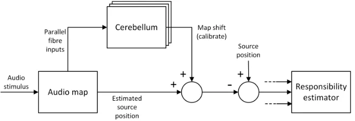
The cerebellar calibration model is an adaptation of that used in a precursory study to that reported here to calibrate whisker input to a robot platform [5], which draws on the adaptive filter model of the cerebellum as shown in Figure 1a. An audio stimulus results in activation of the audio-motor map, which stores a probabilistic representation of the estimated sound source azimuth, generated by the ITD module, in robot head-centric space. The map is divided into a regular grid with activity in each cell of the grid forming one input (i.e. the mossy fibre/parallel fibre) into the cerebellar model. A course-coded version of the map transmits activity at each place on the map to the cerebellum via the parallel fibres. The Purkinje cell, represented by the summing element in Figure 1a, synthesizes the parallel fibre signals modulated by the synaptic weights into a (positive- toward the right, or negative- toward the left) map shift signal that is applied as a bias to the motor output from the audio-motor map. The amount of bias is the weighted sum of the parallel fibre inputs:
δθ=
n
X
i=0
wipi (1)
where n is the number of parallel fibres. The weights wi of the parallel
fibre-Purkinje cell synapses, initially zero, are learnt using the covariance learning rule [12], and updated as in [5]:
∆wi =−βepi (2)
where β is the learning rate, pi the activity on each parallel fibre and e is the
orient error, that is, the difference between the ground truth azimuth of the sound source and the calibrated audio-motor map output.
(a)
(b)
Fig. 1: Cerebellar calibration of audio-motor map. (a) Adaptive filter model of the cerebellum. The audio-motor map stores a probabilistic representation of sound source azimuth in robot head-centric space. A course-coded version of the map transmits activity at each place on the map to the cerebellum via the parallel fibres. The weights wi of the parallel fibre-Purkinje cell synapses are
2.3 Multiple models
A single internal model would need to be very complex in order to capture the range of contexts within which the organism or robot is required to operate as described in section 2.1. This leads to the proposal that the central nervous sys-tem makes use of multiple models each specialized for different contexts [13]. A bio-inspired approach to implementing such models would need a means to select the appropriate model for a particular context. A candidate solution to this problem is the MOdular Selection and Identification for Control [MOSAIC] framework [14, 15]. In this scheme, multiple forward models concurrently pre-dict the consequences of an action (e.g. motor command) and a responsibility predictor attached to the module generates a signal that indicates the degree to which its model is appropriate for the context. The system needs to select the module appropriate to the context by switching the outputs of inverse models on or off. This switching involves two processes [13]:
– the generation of motor commands through the selection of the most appro-priate controller (inverse model) for the estimated context based on sensory input
– a switching process using sensory feedback of the consequences of the action to select a more appropriate model if necessary.
In the original MOSAIC scheme, the inverse models’ contribution is deter-mined through a responsibility signal. This is derived through two further pro-cesses [13]: first, each forward model’s prediction of the next state of the con-trolled system can be compared to the actual state through sensory feedback, but only after the action has taken place (or during action). The second pro-cess estimates responsibility from sensory contextual information, providing the potential to select modules before action.
3
Proposed system
The proposed system is shown in Figure 2. This is a simplification of the mul-tiple models framework, implementing only the models and the responsibility estimator, which simply attempts to identify the most appropriate model for a given context. A more complete system is the subject of current work (section 6). The system has a single ITD module that produces an estimate of sound source azimuth. For the purposes of this study, the ITD module uses a cross-correlation algorithm as described in section 4.2.
which the models learned will be reflected in the different estimates produced. The problem is then one of how to identify the correct context. It is assumed that the model trained in the current context will produce the lowest error in azimuth estimation (of course, this is not always the case, as discussed in section 6). In this study, each prediction is compared to the ground truth position, which is already known from the positioning of the sound source. Although, of course, in the real system, the ground truth cannot be found until the robot head orients toward the sound source, it has been used here merely for convenience to test the efficacy of the approach, and would ultimately be used with visual feedback on a mobile platform. The resulting prediction error is transformed by a psuedo-likelihood function before being normalised across all models using a softmax function as in [13]:
e−|θt−θi|2/σ2
Pn
j=1e−|θt−θj|
2/σ2 (3)
where θt is the ground truth azimuth, θi is the estimate produced by the ith
model,nis the number of estimates (models) andσis a scaling factor which is equivalent to the standard deviation assuming a Gaussian distribution of esti-mates, and is set to unity in this specific configuration. The maximum softmax value corresponds to the lowest error in estimation and is assumed to correctly identify the context. The value ofσ determines the distribution of responsibil-ities across models and has no affect on this identification, and so its value is not important in this particular study (however, it will be important in studies where the outputs of models are to be combined in some way).
4
Method
4.1 Experimental setup
Experiments were automated and controlled using a computer running the Mat-lab environment (The Mathworks Inc.). Algorithms were implemented in the same environment.
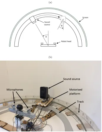
Two microphones (Audio-Technica ATR-3350 omnidirectional condenser lava-lier) were mounted on a horizontal bar with a spacing between centres of 25cm (Figure 3). A relatively large inter-microphone distance was used for the pur-poses of this study in order to achieve a high resolution in the ITD estimation. The microphone bar also had a USB webcam mounted in the centre and was itself mounted on a stepper motor such that it could be oriented toward the estimated sound source azimuth to generate visual feedback of the ground truth position. In the full system, the robot head orients to the estimated azimuth and visual feedback is used to generate the ground truth azimuth. As spatial coordi-nates have an origin at the robot head the system can be transferred to a mobile platform and it is anticipated that such a mobile platform would rotate on a head-centric axis toward the estimated azimuth. However, in this study, for con-venience, the ground truth was taken simply as the randomised set of positions generated for training of the cerebellar models, and the microphone/camera bar remained facing directly ahead.
The sound source was mounted on a motorised platform that could traverse a circular track such that it could be placed (under computer control) at any azimuth between -90o (left with respect to the robot head) and +90o at a con-stant distance from the robot head (Figure 3). A geared stepper motor was used to move the platform and this allowed the source to be placed with a high level of accuracy. 1o increments were used in this study although results are limited by the resolution of the ITD module, which varies from ±1.7o at zero azimuth to ±5o at ±70o azimuth. The resolution is affected by the sampling frequency and inter-microphone distance. The microphones were connected to a computer using a M-Audio MobilePre USB audio capture unit.
The sound source was also mounted on a further stepper motor such that it could be rotated in the transverse plane through an angleφas shown in Figure 3a. This allowed the alteration of the acoustic context by rotation of the sound source so that it might face away at angle φ from the robot head. The exper-imental arena was surrounded by a semi-circular screen that, combined with different orientations of the sound source, produced different acoustic contexts.
4.2 ITD module
The captured audio was processed by the ITD module which used a cross-correlation algorithm to provide an estimate of the azimuth of the location of a sound source:
rlr= n
X
k=0
(a)
(b)
whereRis the right- andLthe left channel audio signal,kis the sample number, n is the current sample and τ is the time lag between left and right channel. The algorithm finds that time difference which results in maximum similarity between the two channels (maximum correlation value), which corresponds to the time difference of arrival of the sound. This was then converted into an estimated azimuth:
θ=180 π sin
−1(cτ dfs
) (5)
where c is the velocity of sound, τ is the estimated ITD, d is the inter-aural distance andfsis the audio sampling frequency.
4.3 Cerebellar models
The cerebellar models were trained in different acoustic contexts. During learn-ing, the robot head was presented with audio from randomised positions along the circular track, such that the direction of arrival of sound was from various azimuths (θin Figure 3a). 60 iterations were used to train a model.
Post learning, all models were presented with the same set of audio stimuli at azimuths from -45o to 45o in 15o increments (some of which may be novel azimuths- i.e. not encountered during training of the cerebellar model). For each stimulus, all models produce a map shift from which a set of errors are derived by computing the difference between each map shift (added to the ITD output) and the ground truth azimuth, and the softmax of the likelihood for each model computed using equation 3. Following the MOSAIC framework, the maximum softmax, corresponding to the minimum error, is used to identify the context.
5
Results
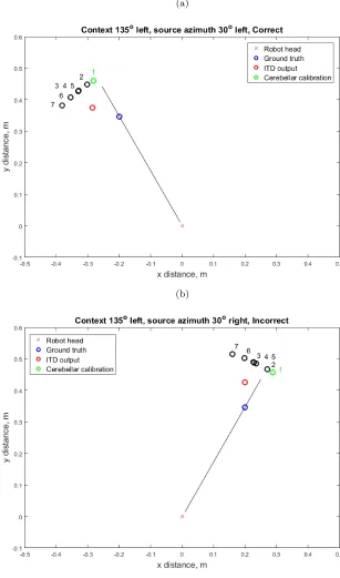
calibration by each of the seven models in one case in which context identifi-cation was correct (Figure 5a) and one case where context identifiidentifi-cation was incorrect (Figure 5b).
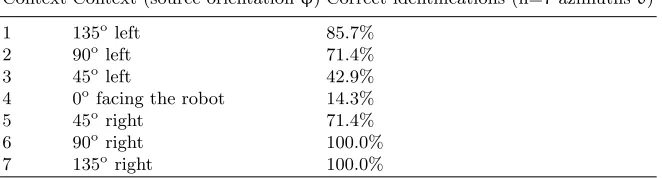
Table 1: Context identification
Context Context (source orientationφ) Correct identifications (n=7 azimuthsθ)
1 135oleft 85.7%
2 90oleft 71.4%
3 45oleft 42.9%
4 0o facing the robot 14.3%
5 45oright 71.4%
(a)
(b)
6
Discussion and future work
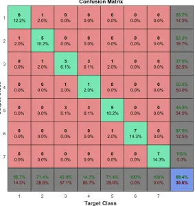
This paper has presented a simple context estimation system which is able to identify the robot’s acoustic context (albeit in a highly constrained way) with a high degree of success, correctly identifying the acoustic context in 69.4% of 49 cases tested. Figure 4 shows that the majority of contexts were correctly iden-tified, and, where mis-classification occurred, this was mostly of a neighbouring (similar) context. The performance of the responsibility estimator varies with the nature of the context. Mis-identification of the context more often occurs where there is little distortion and hence little difference between the model es-timates. This is evident where the sound source directly faced the robot head, so that all models produced similar estimates. The identification rate in this case was only 14.3%, no better than chance. Confusion can also occur where the incorrect model happens to produce a smaller error than the correct model as seen in Figure 5b. Success was greatest where the sound source faced away from the robot head, and there was a clearer distinction between contexts. In terms of localization of the sound source, however, this may not matter, as the goal is to identify the most appropriate model- even if that model did not learn in the presented context. It is anticipated that this technique could be used to augment more classical approaches to sound source localization (including the simple version of ITD used here).
Future work will include mixing model outputs in proportion to their re-sponsibility estimates, and it is anticipated that this will in particular facilitate the adaptation to novel contexts and improve the overall accuracy of the sound source azimuth estimate. This system can only confirm correct model selection after orientation of the robot head (in the real system) to produce a posterior likelihood that the selected model is appropriate. Future work may also include investigation of a responsibility predictor which generates a prior responsibility based on contextual signals. Finally, we wish to investigate to what extent the system could learn de novo, as described in [14].
7
Acknowledgement
The authors wish to thank Ahmad Sheikh for his contribution to developing the moving sound source apparatus.
References
1. S. Argentieri, P. Dan`es, and P. Sou`eres. A survey on sound source localization in robotics: From binaural to array processing methods. Computer Speech & Lan-guage, 34(1):87–112, 2015.
3. John Porrill, Paul Dean, and Sean R. Anderson. Adaptive filters and internal models: Multilevel description of cerebellar function. Neural Networks, 47:134– 149, 2013.
4. John Porrill, Paul Dean, and James V. Stone. Recurrent cerebellar architecture solves the motor-error problem. Proceedings of the Royal Society B: Biological Sciences, 271(1541):789–796, 2004.
5. Tareq Assaf, Emma D. Wilson, Sean Anderson, Paul Dean, John Porrill, and Mar-tin J. Pearson. Visual-tactile sensory map calibration of a biomimetic whiskered robot. In 2016 IEEE International Conference on Robotics and Automation (ICRA), pages 967–972. IEEE, 2016.
6. Jens Blauert. Spatial hearing: the psychophysics of human sound localization, vol-ume Rev. MIT Press, Cambridge, Mass;London;, 1997.
7. Hiroshi Imamizu and Mitsuo Kawato. Cerebellar internal models: Implications for the dexterous use of tools. Cerebellum (London, England), 11(2):325–335, 2012. 8. Oliver Baumann, Ronald Borra, James Bower, Kathleen Cullen, Christophe Habas,
Richard Ivry, Maria Leggio, Jason Mattingley, Marco Molinari, Eric Moulton, Michael Paulin, Marina Pavlova, Jeremy Schmahmann, and Arseny Sokolov. Con-sensus paper: The role of the cerebellum in perceptual processes. Cerebellum, 14(2):197–220, 2015.
9. M. Fujita. Adaptive filter model of the cerebellum. Biol Cybern, 45(3):195–206, 1982.
10. David Marr. A theory of cerebellar cortex.The Journal of Physiology, 202(2):437– 470.1, 1969.
11. James S. Albus. A theory of cerebellar function. Mathematical Biosciences, 10(12):25–61, 1971.
12. T. J. Sejnowski. Storing covariance with nonlinearly interacting neurons. J Math Biol, 4(4):303–21, 1977.
13. D. M. Wolpert and M. Kawato. Multiple paired forward and inverse models for motor control. Neural Networks, 11(78):1317–1329, 1998.
14. Masahiko Haruno, Daniel M. Wolpert, and Mitsuo Kawato. Mosaic model for sensorimotor learning and control. Neural Computation, 13(10):2201–2220, 2001. 15. Norikazu Sugimoto, Masahiko Haruno, Kenji Doya, and Mitsuo Kawato. Mosaic