On Using The Median Ranked Set Sampling for Developing Reliability Test Plans Under Generalized Exponential Distribution

On Using the Median Ranked Set Sampling for Developing

Reliability Test Plans Under Generalized Exponential Distribution

Amjad D. Al-Nasser

Department of Statistics, Science Faculty, Yarmouk University, Irbid, Jordan [email protected]

Fatima S. Abdullah

Department of Mathematics, Science Faculty, Hadhramout University, Mukalla, Yemen [email protected]

Abstract

In this article a new single sampling plan based on ranked data scheme is proposed. Two main requirements are considered for the new plan: the lifetime of the test units is assumed to follow the generalized exponential distribution; and the data are selected by using the median ranked set sampling scheme from a large lot. The distribution function characterization under the median ranked set sampling scheme is derived assuming that the set size is known; the minimum number of set cycle and consequently the minimum sample size necessary to ensure the specified average life are obtained and the operating characteristic values of the ranked sampling plans as well as the producer’s risk are presented. An illustrative examples based on the results obtained are given.

Mathematics Subject Classifications: 60D05, 62G30

Keywords: Median Ranked Set Sampling, Acceptance Sampling Plans, Generalized exponential Distribution, Operating Characteristic Function Value, Producer's Risk, Consumer's Risk.

1. Introduction

Several authors modified the RSS scheme, usually the modification on the ranked sampling scheme based on a new criterion to assign the location of the selected item within the second stage of the novel RSS scheme (Samawi et al., 1996; Muttlak, 1997; Muttlak, 2003; Jemain and Al-Omari, 2006; Al-Nasser, 2007, Al-Nasser and Bani Mustafa, 2009; and Al-Nasser and Al-Omari, 2015). Unlike of the modification of RSS, the main aim of this article is to use the RSS in acceptance sampling research area rather than improving the RSS scheme. Mainly, an interesting ranked data sampling schemes proposed by Muttlak (1997) and known by the median ranked set sampling (MRSS) will be considered and used in this article. The main advantages of MRSS are the ability of error in ranking reduction and the ability of increasing the efficiency of the estimator. The MRSS method as given by Muttlak (1997) can be summarized as follows:

Step.1 Select m random samples "sets" each of size m from a given population.

Step.2 Rank the items within each set with respect to a variable of interest by any cost free method.

Step.3 If the set size m is odd, then select for measurement the (m+1₂ ) th

smallest rank (the median) from each set for actual measurement.

Step.4 If the set size m is even, then select for measurement from the first m/2 samples the (m₂)

th

smallest rank; and from the second m/2 samples select the (m+2₂ )th smallest for actual measurement.

Step.5 The cycle may be repeated r times (i.e. r is number of cycles) to obtain the desired sample size n = m ∗ r.

Now, assume that 𝑋₁, 𝑋₂, … , 𝑋_𝑛 be a SRS of size n having a probability density function (pdf) f(x) and cumulative distribution (CDF) F(x) with finite mean 𝜇 and finite variance 𝜎2_{. Consequently, and based on the MRSS steps; the element of the desired MRSS} sample will be in the form:

{ {𝑋_[𝑚+1

2 :𝑚]𝑖𝑗; 𝑖 = 1,2, … , 𝑚, 𝑗 = 1,2, … , 𝑟} 𝑚 𝑖𝑠 𝑜𝑑𝑑

{(𝑋_[𝑚

2:𝑚]𝑖𝑗, 𝑋[ 𝑚+2

2 :𝑚]𝑘𝑗) ; 𝑖 = 1,2, … ,

𝑚 2 ; 𝑘 =

𝑚

2 + 1, … , 𝑚, 𝑗 = 1,2, … , 𝑟} ; 𝑚 𝑖𝑠 𝑒𝑣𝑒𝑛

where 𝑋_[𝑚+1 2 :𝑚]𝑖𝑗

is the (𝑚+1 2 )

𝑡ℎ

judgment order statistics of the 𝑖𝑡ℎ random sample of size m in the 𝑗𝑡ℎ cycle. It should be noted that all of 𝑋_[𝑚+1

2 :𝑚]𝑖𝑗

's are mutually independent and identically distributed. Now, based on MRSS scheme the 𝑑𝑓, in general, will be:

𝑓_{𝑀𝑅𝑆𝑆}(𝑥) =

{ 1

𝑟𝑚∑ ∏ 𝑓𝑋(𝑚+1_{2 )𝑖}(𝑥)

𝑚 𝑖=1 𝑟

𝑗=1 , if 𝑚 is odd

1

𝑟𝑚∑ ∏ (𝑓𝑋(𝑚_{2 )𝑖}(𝑥) + 𝑓𝑋(𝑚+2_{2 )𝑖}(𝑥))

𝑚/2 𝑖=1 𝑟

𝑗=1 , if 𝑚 is even

equivalently to:

𝑓_{𝑀𝑅𝑆𝑆}(𝑥) =

{

∏ 𝑓_𝑋

(𝑚+1_{2 )𝑖}(𝑥)

𝑚

𝑖=1 , if 𝑚 is odd

∏ (𝑓𝑋₍𝑚 2 )𝑖

(𝑥) + 𝑓𝑋

(𝑚+2_{2 )𝑖}(𝑥))

𝑚/2

𝑖=1 , if 𝑚 is even

(1)

David and Nagaraja (2003), showed that the 𝑝𝑑𝑓 of the 𝑖𝑡ℎ order statistic is given by:

𝑓𝑋_(𝑖)(𝑥) =

𝑛!

(𝑖 − 1)! (𝑛 − 𝑖)!(𝐹(𝑥)) 𝑖−1

(1 − 𝐹(𝑥))𝑛−𝑖𝑓(𝑥), −∞ < 𝑥 < ∞

Therefore,

𝑓_{𝑀𝑅𝑆𝑆}(𝑥) =(2𝑚∗+ 1)!

(𝑚∗_!)2 (𝐹(𝑥)) 𝑚∗

(1 − 𝐹(𝑥))𝑚∗𝑓(𝑥)

where

𝑚∗_{= {} 𝑚−1

2 , if 𝑚 is odd

𝑚

2 − 1, if 𝑚 is even .

and the corresponding 𝑐𝑑𝑓 will be 𝐹_{𝑀𝑅𝑆𝑆}(𝑥) = ∫ 𝑓₋𝑥_{∞ 𝑀𝑅𝑆𝑆}(𝑡)𝑑𝑡; which equivalent to:

𝐹

(𝑥) = ∑

(

) (𝐹(𝑥))

(1 − 𝐹(𝑥))

2𝑚∗+1

𝑗=𝑚∗₊₁ (2)

The majority of research of ranked data has been concerned with estimating the population mean. However, none of the previous research considered any of the RSS concepts in the acceptance sampling context, this article could be consider as a new contribution in this practical research area. Acceptance sampling is an important application in the quality control field, which can be considered as a test procedure, the first time this statistical procedure is used by the United State military to test bullets before shipping during the World War II. Later, used in many fields such as medical and manufacturing.

The procedure of the classical single acceptance sampling plan (ASP) based on SRS consists of the following steps:

Step.1 Draw a SRS of size n items from a large lot

Step.2 Classify each item within the selected sample as defective or non-defective item.

Step.3 If the number of defective items exceed the acceptance number (c), then the entire lot is rejected; otherwise it is accepted.

2003; Baklizi and El Masri, 2004; Balakrishnan, et al, 2007; Rao, 2009; Aslam et al, 2010; Al-Omari, 2014 and Al-Omari, 2015). Usually, with every ASP(n, c), the problem is to find the unknown parameters n and c that satisfies:

𝑃(𝑋 ≤ 𝑐|𝑛, 𝑝₁) = 1 − 𝛼∗

𝑃(𝑋 ≤ 𝑐|𝑛, 𝑝2) = 𝛽

} (3)

where 𝛼∗ is the Type I error; the probability a good lot is rejected (producer's risk) and 𝛽 is the Type II error (consumer's risk) which is the probability that a bad lot is accepted. Moreover, 𝑝₁ is the acceptable quality limit (AQL) and 𝑝₂ is the lot tolerance percent defective (LTPD). Computing the probabilities in (3) depends on the lot size, when the sampling from isolated lot size then the Hyper-geometric distribution is employed, however, if the lot size is large enough, then Binomial distribution is employed. Moreover, a lifetime distribution for the quality characteristic is assumed such as the generalized exponential distribution; to obtain AQL and LTDP; then based on the given distribution the minimum sample size (n) that needed to ensure a certain mean life for an items in the lot is obtained under the assumption that the experiment should be terminated a predetermined time, say t.

The problem that we are introducing in this article is to consider the MRSS in selecting the items from a large lot assuming that the underling lifetime distribution is the generalized exponential distribution. The main idea of using MRSS in acceptance sampling context is to decrease the producer risk that rises when the items selected by the typical ASP(n, c) based on a SRS techniques.

The remainder of the paper is organized as follows. In section 2, summarizes the acceptance sampling assumptions and the notations that will be used through this article. Section.3 illustrate the generalized exponential distribution characterizations under the MRSS scheme. Section.4 introduces the proposed acceptance sampling plan and the operating characteristic function. The results and a descriptive example are given in section 5. A comparisons between acceptance sampling plan based on SRS and MRSS is given in section.6. The article ends with concluding remarks and suggested future research in section 7.

2. Notations and Acceptance Sampling Assumptions

The single acceptance sampling for attributes problems is developed with the following notations and assumptions:

i. The lifetime is following a generalized exponential distribution (𝐺𝐸(𝛼, 𝜆)), with the following probability density function 𝑝𝑑𝑓 and cumulative distribution function 𝑐𝑑𝑓, respectively:

𝑓(𝑥; 𝛼, 𝜆) = 𝛼_𝜆(1 − 𝑒−𝑥 𝜆⁄ ₎𝛼−1_𝑒−𝑥 𝜆⁄ _{, 𝑥 > 0, 𝜆 > 0, 𝛼 > 0 (4)}

ii. where 𝛼 is the shape parameter and 𝜆 is the scale parameter. iii. The MRSS will be used to select a random samples from a lot. iv. 𝛼∗ is the producer's risk

v. 𝛽 is the consumer's risk

vi. m is the set is in the ranked data scheme

vii. r is the number of independent samples; or number of cycles in the ranked data scheme

viii. n is the sample size

ix. c is the acceptance number, if number of defective items is less than or equal to c in a given time interval then the Lot has acceptable quality.

x. ASP, single acceptance sampling plan based on SRS. xi. ASPmed, single acceptance sampling plan based on MRSS. xii. 𝜇0 is the true mean life of a given product.

3. Characterization of the Generalized Exponential Distribution Under MRSS

The generalized exponential distribution (GED) given in (4) has been introduced by Gupta and Kundu (1999). Recently, it is observed that the generalized exponential distribution has been used quite effectively to analyze lifetime data. In many cases it is observed that it provides a better fit than the Weibull, gamma, log-normal or generalized Rayleigh distributions Aslam et al (2010). Accordingly, Aslam and Shajbaz (2007), developed an economic reliability acceptance sampling plans when the lifetime follows a generalized exponential distribution. In this section, the generalized exponential distribution will be re characterized based on the MRSS. Consequently, the 𝐺𝐸(𝛼, 𝜆) is given in (4) and (5), and by using the 𝑝𝑑𝑓 and 𝑐𝑑𝑓 based on the MRSS as given in (1) and (2), then the new characterization of the distribution will be:

𝑓𝑀𝑅𝑆𝑆(𝑥; 𝛼, 𝜆) = 𝛼 𝜆

(2𝑚∗_{+ 1)!}

𝜆(𝑚∗_!)2 (1 − 𝑒−𝑥 𝜆⁄ )

𝛼(𝑚∗+1)−1

(1 − (1 − 𝑒−𝑥 𝜆⁄ ₎𝛼₎𝑚∗

𝐹_{𝑀𝑅𝑆𝑆}(𝑥; 𝛼, 𝜆) = ∑ (2𝑚∗+ 1

𝑗 ) (1 − 𝑒−𝑥 𝜆⁄ ) 𝛼𝑗

(1 − (1 − 𝑒−𝑥 𝜆⁄ ₎𝛼₎2𝑚∗+1−𝑗 2𝑚∗₊₁

𝑗=𝑚∗₊₁

Figure. 1: The 𝒑𝒅𝒇 of 𝑮𝑬(𝜶, 𝝀) based on MRSS with 𝒎 = 𝟏 and 𝝀 = 𝟐.

Figure. 2: The 𝒄𝒅𝒇 of 𝑮𝑬(𝜶, 𝝀) based on MRSS with 𝒏 = 𝟑 and 𝝀 = 𝟐.

The mean lifetime based on MRSS is:

𝜇 = ∫ 𝑥𝛼 𝜆

(2𝑚∗_{+ 1)!}

𝜆(𝑚∗_!)2 (1 − 𝑒−𝑥 𝜆⁄ )

𝛼(𝑚∗+1)−1

(1 − (1 − 𝑒−𝑥 𝜆⁄ ₎𝛼₎𝑚∗_𝑑𝑥

∞

0

= 𝜆(2𝑚∗+ 1)!

(𝑚∗_!)2 ∑ [(−1)𝑖( 𝑚∗

𝑖 ) (

𝐻_𝛼(𝑚∗_+𝑖+1)

𝑚∗_{+ i + 1})] 𝑚∗

𝑖=0

Where 𝐻_(𝑢) is the Harmonic Number (Raqab and Ahsanullah (2001)) which defined as:

𝐻_(𝑢) = ∑ 1 𝑗⁄ 𝑢

𝑗=1 ;

hence,

𝜇 = 𝜆(2𝑚∗+ 1)! (𝑚∗_!)02 ∑ [

(−1)𝑖₍𝑚∗

𝑖 )

𝑚∗_{+ i + 1} ∑ (1 𝑗⁄ ) 𝛼(𝑚∗_+𝑖+1)

𝑗=1

] 𝑚∗

𝑖=0

where k =(2𝑚 ∗_{+ 1)!}

(𝑚∗_!)2 ∑ [

(−1)𝑖₍𝑚∗

𝑖 )

𝑚∗_{+ i + 1} ∑ (1 𝑗⁄ ) 𝛼(𝑚∗_+𝑖+1)

𝑗=1

] 𝑚∗

𝑖=0

4. Design of the Ranked Acceptance Sampling Plan

It is assumed that the truncated life test is conducted when the lifetime of the product follows a generalized exponential distribution as defined in (4). The item from a large lot will be selected using the MRSS scheme. The life test terminates at a pre-assigned time 𝑡₀ and the number of failures during this time interval [0, 𝑡] is recorded. The decision to accept the lot occurs if and only if the recorded number of failures at the end of the time point 𝑡₀ is less than or equal to the acceptance number 𝑐. The lot size is assumed infinitely large enough so that the theory of the binomial distribution is applied. The acceptance or rejection of the lot is equivalent to the acceptance or rejection of the hypothesis 𝐻₀ ∶ 𝜇 ≥ 𝜇₀. For the sake of convenience, set the termination time as a multiple of the specified mean lifetime; that is, 𝑡₀ = 𝑑𝜇₀, where d is a positive constant. The proposed acceptance sampling plan is characterized by ASPmed(r, m, 𝑐), which consists of:

• Drawing r MRSS each of size m and put them on a test during time 𝑡₀.

• Accept the lot, if there are no more than or equal to c failures; However, reject the lot and terminated sampling immediately, if (c+1) defective items are discovered in the first n = r × m; items.

The consumer risk is fixed such that it does not exceed 1 − 𝑃∗:

∑ (𝑟𝑚

𝑖 ) 𝑝𝑖(1 − 𝑝)𝑟𝑚−𝑖 𝑐

𝑖=0

≤ 1 − 𝑃∗ ₍₅₎

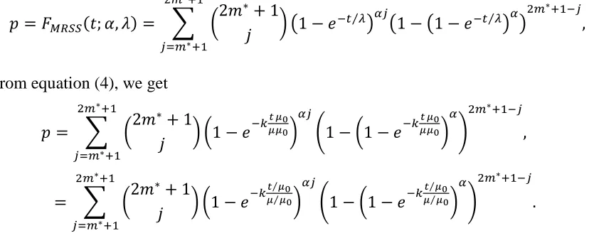
where 𝑝 = 𝐹(𝑡; 𝜆) considered as a function of λ0.

𝑝 = 𝐹𝑀𝑅𝑆𝑆(𝑡; 𝜆0) = ∑ (

2𝑚∗_{+ 1}

𝑗 ) (1 − 𝑒−𝑡 𝜆⁄ 0) 𝛼𝑗

(1 − (1 − 𝑒−𝑡 𝜆⁄ 0)𝛼)2𝑚 ∗_+1−𝑗

2𝑚∗₊₁

𝑗=𝑚∗₊₁

,

From equation (4), we get

𝑝 = ∑ (2𝑚

∗_{+ 1}

𝑗 ) (1 − 𝑒 −𝑘_𝜇0𝑡

) 𝛼𝑗

(1 − (1 − 𝑒−𝑘𝜇0𝑡 ₎

𝛼 )

2𝑚∗+1−𝑗 2𝑚∗₊₁

𝑗=𝑚∗₊₁

,

The minimum values of 𝑛 = 𝑟𝑚 satisfying inequality (5) are obtained for fixed set size 𝑚 = 3, 4, 5 and 6 and given in Table.1 and Table.2. Also, we set 𝑝∗ = 0.75, 0.9, 0.95, 0.99, and _𝜇𝑡

0 = 0.628, 0.942, 1.257, 1.571, 2.356, 3.141, 3.927, 4.712. This choice is

consistent with that of Baklizi et al. (2005), Al-Nasser and Al-Omari (2013); and Kantam and Rosaiah (1998, 2001). The operating characteristic values of the sampling plan (r,

𝑚∗_,c,𝑡

𝜇0) gives the probability of accepting the lot. This probability is given by

𝐿(𝑝) = ∑ (𝑟𝑚∗

𝑖 ) 𝑝𝑖(1 − 𝑝)𝑟𝑚

∗_−𝑖

𝑐

𝑖=0

where pF









𝑝 = 𝐹_{𝑀𝑅𝑆𝑆}(𝑡; 𝛼, 𝜆) = ∑ (2𝑚∗_𝑗+ 1) (1 − 𝑒−𝑡 𝜆⁄ ₎𝛼𝑗_{(1 − (1 − 𝑒}−𝑡 𝜆⁄ ₎𝛼₎2𝑚∗+1−𝑗 2𝑚∗₊₁

𝑗=𝑚∗₊₁

,

From equation (4), we get

𝑝 = ∑ (2𝑚∗+ 1

𝑗 ) (1 − 𝑒 −𝑘_𝜇𝑡𝜇0

𝜇0)

𝛼𝑗

(1 − (1 − 𝑒−𝑘𝜇𝑡𝜇0_𝜇0)

𝛼 )

2𝑚∗_+1−𝑗

2𝑚∗₊₁

𝑗=𝑚∗₊₁

,

= ∑ (2𝑚

∗_{+ 1}

𝑗 ) (1 − 𝑒 −𝑘_{𝜇 𝜇0}𝑡 𝜇0⁄_⁄

) 𝛼𝑗

(1 − (1 − 𝑒−𝑘𝜇 𝜇0𝑡 𝜇0⁄⁄ ₎

𝛼 )

2𝑚∗+1−𝑗 2𝑚∗₊₁

𝑗=𝑚∗₊₁

.

The producer’s risk is the probability of rejecting the lot when ₀. Under the sampling plan under consideration, and given a value for the producer’s risk, say 0.05, one may be interested in knowing what value of 𝜇 𝜇⁄ ₀will ensure the producer’s risk less than or equal to 0.05. This value of 𝜇 𝜇⁄ ₀is the smallest number 𝜇 𝜇⁄ ₀for which 𝐹((𝑡 𝜇⁄ )/(𝜇 𝜇0 ⁄ ))0 satisfies the inequality

∑ (𝑟𝑚∗

𝑖 ) 𝑝𝑖(1 − 𝑝)𝑟𝑚

∗_−𝑖

𝑐

𝑖=0

≥ 0.95 (7)

For a given sampling plan (r, 𝑚∗,c,_𝜇𝑡

0) at specified confidence level 𝑝

∗ _{the minimum}

values of 𝜇 𝜇⁄ ₀ satisfying inequality (7) are computed and presented in Table.5 and Table.6.

5. Illustrative Examples

For example, assume that an experimenter wants to establish the true mean life to be at least 𝜇₀ = 1000 hours with confidence level 𝑝∗ = 0.95, and the experiment will be stopped at 𝑡 = 942 hours. when the acceptance number 𝑐 = 2, then by using MRSS scheme there are several acceptance sampling plans obtained, hence, the required sample size 𝑛 from Table.1 and Table.2 depends on number of cycles:

Table 7: Minimum sample size for median ranked acceptance sampling plan

ASPmed(r, 𝑚∗ ,c) Minimum sample size

ASPmed(4, 3, 2) 12

ASPmed(3, 4, 2) 12

ASPmed(3, 5, 2) 15

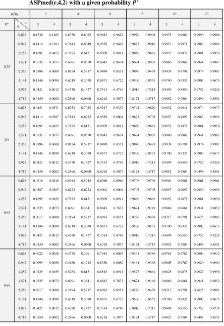
Now, for any of the above sampling plans; the minimum number of items have to be inspected during 1000 hours, if the producer couldn’t observe 2 defective items out of the sample, then the experimenter can assert with confidence 0.95 that the mean life is at least 1000 hours. For the suggested sampling plans given in Table.1 and Table.2, when the specified mean life is 0.942; the operating characteristic values from Table.3 and Table.4 are:

Table 8: Selected operating characteristic values for median ranked acceptance sampling plan

𝜇 𝜇⁄ 0 2 4 6 8 10 12

ASPmed(4, 3, 2) 0.0387 0.6222 0.9004 0.9705 0.9897 0.9959

ASPmed(3, 4, 2) 0.0387 0.6222 0.9004 0.9705 0.9897 0.9959

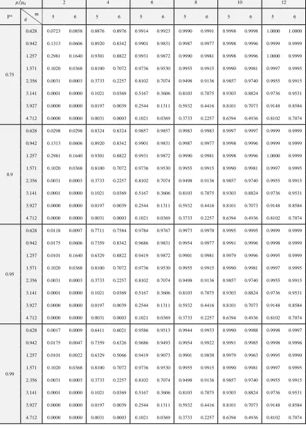
ASPmed(3, 5, 2) 0.0175 0.7359 0.9686 0.9954 0.9991 0.9998

ASPmed(2, 6, 2) 0.0606 0.8342 0.9831 0.9977 0.9996 0.9999

This means that; for ASPmed(4,3,2); if the true mean life is twice the specified mean life (𝜇 𝜇⁄ ₀ = 2) then the producer's risk is about 1 − 0.0387 = 0.9613.

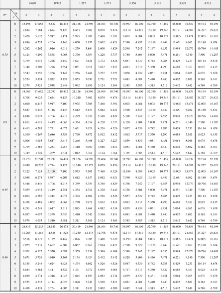
From Table 3, we can get the value of𝜇 𝜇⁄ ₀ for several values of the other sampling plan parameters such that the producer risk less than 0.05. Under the above example; ASPmed(4, 3, 2) and 𝑝∗ = 0.95; the value of 𝜇 𝜇⁄ ₀ = 7.100. This means that the product can have an average life of 7.100 times the specified average lifetime of 1000 hours in order that the product be accepted with probability at least 0.95.

6. Comparison Between ASPmed(r, m, c) and ASP(n, c)

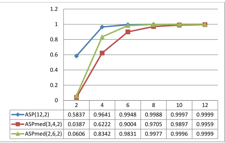
Figure 3: Operating Characteristic Values Comparisons between SRS and MRSS Sampling Plans

7. Concluding Remarks

In this paper, we have proposed a ranked data single sampling plan. Tables have been constructed for the easy selection of the optimal plan parameters when the lifetime of the product follows the generalized distribution. The proposed plan performs better than the reference plan in terms of sample size. The proposed plan can be extended by using different sampling scheme such as ranked set sampling. extreme ranked set sampling as future research.

Acknowledgements

The authors would like to thank the Journal editorial board and the referees for several valuable comments.

References

1. Al-Nasser, A.D. and Al-Omari, A.I. (2013). Acceptance sampling plan based on truncated life tests for exponentiated Frechet distribution. Journal of Statistics and Management Systems, 16(1): 13-24.

2. Al-Nasser, A.D. and Al-Omari, A. (2015). Information Theoretic Weighted Mean Based on Truncated Ranked Set Sampling. Journal of Statistical Theory and Practice. 9(2): 313- 329.

3. Al-Nasser, A.D. (2007). L ranked set sampling: a generalization procedure for robust visual sampling. Communication in Statistics-Simulation and Computation, 36, 33–44.

2 4 6 8 10 12

ASP(12,2) 0.5837 0.9641 0.9948 0.9988 0.9997 0.9999

ASPmed(3,4,2) 0.0387 0.6222 0.9004 0.9705 0.9897 0.9959

ASPmed(2,6,2) 0.0606 0.8342 0.9831 0.9977 0.9996 0.9999

4. Al-Nasser, A.D. and Bani-Mustafa, A. (2009). Robust extreme ranked set sampling. Journal of Statistical Computation and Simulation 79, 859–867.

5. Al-Omari, A.I. (2014). Acceptance sampling plan based on truncated life tests for three parameter kappa distribution. Economic Quality Control, 29(1): 53-62. 6. Al-Omari, A.I. (2015). Time truncated acceptance sampling plans for generalized

inverted exponential distribution. Electronic Journal of Applied Statistical Analysis, 8(1): 1-12.

7. Aslam M., Kundu D., and Ahmad M. (2010). Time truncated acceptance sampling plans for generalized exponential distribution. Journal of Applied Statistics, 37(4): 555–566.

8. Aslam, M., Azam, M., Lio, Y.L., Jun, C.-H. (2013). Two-stage group acceptance sampling plan for Burr Type X percentiles. J. Test. Eval. 41 (4): 525–533.

9. Aslam, M., and Shahbaz M. (2007). Economic Reliability Test Plans using the Generalized Exponential Distribution. Journal of Statistics, 14, 53-60.

10. Baklizi, A. (2003). Acceptance sampling based on truncated life tests in the Pareto distribution of the second kind. Advances and Applications in Statistics, 3(1): 33-48.

11. Baklizi, A. and El Masri, A. (2004) Acceptance sampling based on truncated life tests in the Birnbaum–Saunders model. Risk Analysis. Vol. 24, 2004, pp. 1453– 1457.

12. Baklizi, A., El Masri, A. and Al-Nasser, A.D. (2005). Acceptance sampling plans in the Rayleigh model. The Korean Communications in Statistics, 12(1): 11-18. 13. Balakrishnan, N, Leiva, V. and López, J. (2007). Acceptance sampling plans from

truncated life tests based on the Generalized Birnbaum–Saunders distribution. Communications in Statistics-Simulation and Computation, 36: 643–656.

14. Chen, Z., Bai, Z.D. and Sinha, B.K. (2004). Ranked set sampling: Theory and applications. Springer-Verlag New York, Inc.

15. David, H., and Nagaraja H. (2003). Order Statistics, 3rd ed., John Wiley & Sons, Inc., New Jersey.

16. Epstein, B. (1954). Truncated life tests in the exponential case. The Annals of Mathematical Statistics, 25:555-564.

17. Gulati, S. (2004). Smooth non-parametric estimation of the distribution function from balanced ranked set samples. Environmetrics, 15, 529–539.

18. Gupta, R.D. and Kundu, D. (1999). Generalized exponential distribution. Austral and New Zealand Journal of statistics., 41(2): 173-188.

19. Jemain A., and Al-Omari A. (2006). Double quartile ranked set samples. Pakistan Journal of Statistics 22 (2006), 217–228.

21. Kantam, R.R.L. and Rosaiah, K. (1998). Half logistic distribution in acceptance sampling based on life tests. Indian Association for Productivity, Quality and Reliability (IAPQR) Transactions, 23(2): 117-125.

22. Kantam, R.R.L., Rosaiah, K., and Rao, G.S. (2001). Acceptance sampling based on life tests: log-logistic models, Journal of applied statistics., 28 (1): pp 121 – 128.

23. McIntyre, G. A. (1952). A method of unbiased selective sampling using ranked sets. Australian J. Agricultural Research. 3, 385-390.

24. Muttlak, H. (1997). Median ranked set sampling. J. Appl. Statist. Sci. 6. 245-255. 25. Muttlak, H. (2003). Modified Ranked set Sampling. Pak. J. Statistics 19. 3(4):

315-323.

26. Rao, S. (2009). A group acceptance sampling plans for lifetimes following a generalized exponential distribution. Economic Quality Control, 24(1), 75–85. 27. Raqab, M., Ahsanullah, M. (2001). Estimation of the location and scale

parameters of eneralized exponential distribution based on order statistics. J. Statist. Comp. Simul. 69:109–123.

28. Samawi, H. Abu-Dayyeh, W and Ahmed, M. S. (1996). Estimating the population mean using extreme ranked set sampling. Biometrical Journal. 38. 577-586. 29. Samuh, Monjed H. and Qtait, Areen (2015) "Estimation for the Parameters of the

Exponentiated Exponential Distribution Using a Median Ranked Set Sampling," Journal of Modern Applied Statistical Methods, 14: 1, 215-237.

30. Sinha, B. K., Sinha, B. K., and Purkayastha, S. (1996).On some aspects of ranked set sampling for estimation of normal and exponential parameters. Statist. Decisions 14 223–240.

31. Sobel, M., and Tischendrof, J.A. (1959). Acceptance sampling with new life test objectives. Proceedings of the fifth national symposium on reliability and quality control, Philadelphia, Pennsylvania, 108 – 118.

32. Stokes, S. L. and Sager, T.W. (1988). Characterization of a ranked-set sample with application to estimating distribution function. Journal of the American Statistical Association, 83, 374–381.

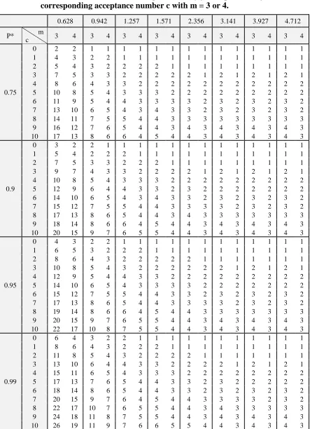
Table 1: Necessary number of cycles ( r ) in MRSS sampling scheme need to ensure the mean life exceeds a given value 𝝁_𝟎 with probability 𝑷∗ and the corresponding acceptance number c with m = 3 or 4.

0.628 0.942 1.257 1.571 2.356 3.141 3.927 4.712

P* m

c 3 4 3 4 3 4 3 4 3 4 3 4 3 4 3 4

0.75

0 2 2 1 1 1 1 1 1 1 1 1 1 1 1 1 1

1 4 3 2 2 1 1 1 1 1 1 1 1 1 1 1 1

2 5 4 3 2 2 2 2 1 1 1 1 1 1 1 1 1

3 7 5 3 3 2 2 2 2 2 1 2 1 2 1 2 1

4 8 6 4 3 3 2 2 2 2 2 2 2 2 2 2 2

5 10 8 5 4 3 3 3 2 2 2 2 2 2 2 2 2

6 11 9 5 4 4 3 3 3 3 2 3 2 3 2 3 2

7 13 10 6 5 4 3 4 3 3 2 3 2 3 2 3 2

8 14 11 7 5 5 4 4 3 3 3 3 3 3 3 3 3

9 16 12 7 6 5 4 4 3 4 3 4 3 4 3 4 3

10 17 13 8 6 6 4 5 4 4 3 4 3 4 3 4 3

0.9

0 3 2 2 1 1 1 1 1 1 1 1 1 1 1 1 1

1 5 4 2 2 2 1 1 1 1 1 1 1 1 1 1 1

2 7 5 3 3 2 2 2 1 1 1 1 1 1 1 1 1

3 9 7 4 3 3 2 2 2 2 1 2 1 2 1 2 1

4 10 8 5 4 3 3 3 2 2 2 2 2 2 2 2 2

5 12 9 6 4 4 3 3 2 3 2 2 2 2 2 2 2

6 14 10 6 5 4 3 4 3 3 2 3 2 3 2 3 2

7 15 12 7 5 5 4 4 3 3 3 3 2 3 2 3 2

8 17 13 8 6 5 4 4 3 4 3 3 3 3 3 3 3

9 18 14 8 6 6 4 5 4 4 3 4 3 4 3 4 3

10 20 15 9 7 6 5 5 4 4 3 4 3 4 3 4 3

0.95

0 4 3 2 2 1 1 1 1 1 1 1 1 1 1 1 1

1 6 5 3 2 2 2 1 1 1 1 1 1 1 1 1 1

2 8 6 4 3 2 2 2 2 2 1 1 1 1 1 1 1

3 10 8 5 4 3 2 2 2 2 2 2 1 2 1 2 1

4 12 9 5 4 4 3 3 2 2 2 2 2 2 2 2 2

5 14 10 6 5 4 3 3 3 3 2 2 2 2 2 2 2

6 15 12 7 5 5 4 4 3 3 2 3 2 3 2 3 2

7 17 13 8 6 5 4 4 3 3 3 3 2 3 2 3 2

8 19 14 8 6 6 4 5 4 4 3 3 3 3 3 3 3

9 20 15 9 7 6 5 5 4 4 3 4 3 4 3 4 3

10 22 17 10 8 7 5 5 4 4 3 4 3 4 3 4 3

0.99

0 6 4 3 2 2 1 1 1 1 1 1 1 1 1 1 1

1 8 6 4 3 2 2 2 1 1 1 1 1 1 1 1 1

2 11 8 5 4 3 2 2 2 2 1 1 1 1 1 1 1

3 13 10 6 4 4 3 3 2 2 2 2 1 2 1 2 1

4 15 11 6 5 4 3 3 3 2 2 2 2 2 2 2 2

5 17 13 7 6 5 4 4 3 3 2 3 2 2 2 2 2

6 18 14 8 6 5 4 4 3 3 2 3 2 3 2 3 2

7 20 15 9 7 6 4 5 4 4 3 3 3 3 2 3 2

8 22 17 10 7 6 5 5 4 4 3 4 3 3 3 3 3

9 24 18 11 8 7 5 5 4 4 3 4 3 4 3 4 3

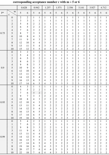
Table 2: Necessary number of cycles ( r ) in MRSS sampling scheme need to ensure the mean life exceeds a given value 𝝁_𝟎 with probability 𝑷∗ and the corresponding acceptance number c with m = 5 or 6

0.628 0.942 1.257 1.571 2.356 3.141 3.927 4.712

P* m

c 5 6 5 6 5 6 5 6 5 6 5 6 5 6 5 6

0.75

0 2 2 1 1 1 1 1 1 1 1 1 1 1 1 1 1

1 3 3 1 1 1 1 1 1 1 1 1 1 1 1 1 1

2 5 4 2 2 1 1 1 1 1 1 1 1 1 1 1 1

3 6 5 2 2 2 1 1 1 1 1 1 1 1 1 1 1

4 7 6 3 2 2 2 2 1 1 1 1 1 1 1 1 1

5 8 7 3 3 2 2 2 2 2 1 2 1 2 1 2 1

6 10 8 4 3 2 2 2 2 2 2 2 2 2 2 2 2

7 11 9 4 3 3 2 2 2 2 2 2 2 2 2 2 2

8 12 10 4 4 3 3 2 2 2 2 2 2 2 2 2 2

9 13 11 5 4 3 3 3 2 2 2 2 2 2 2 2 2

10 15 12 5 5 4 3 3 3 3 2 3 2 3 2 3 2

0.9

0 3 2 1 1 1 1 1 1 1 1 1 1 1 1 1 1

1 5 4 2 2 1 1 1 1 1 1 1 1 1 1 1 1

2 6 5 2 2 1 1 1 1 1 1 1 1 1 1 1 1

3 8 6 3 2 2 2 1 1 1 1 1 1 1 1 1 1

4 9 8 3 3 2 2 2 2 1 1 1 1 1 1 1 1

5 10 9 4 3 2 2 2 2 2 1 2 1 2 1 2 1

6 12 10 4 4 3 2 2 2 2 2 2 2 2 2 2 2

7 13 11 5 4 3 3 2 2 2 2 2 2 2 2 2 2

8 14 12 5 4 3 3 3 2 2 2 2 2 2 2 2 2

9 16 13 6 5 4 3 3 2 2 2 2 2 2 2 2 2

10 17 14 6 5 4 3 3 3 3 2 3 2 3 2 3 2

0.95

0 4 3 1 1 1 1 1 1 1 1 1 1 1 1 1 1

1 5 5 2 2 1 1 1 1 1 1 1 1 1 1 1 1

2 7 6 3 2 2 1 1 1 1 1 1 1 1 1 1 1

3 9 7 3 3 2 2 2 1 1 1 1 1 1 1 1 1

4 10 8 4 3 2 2 2 2 1 1 1 1 1 1 1 1

5 12 10 4 3 3 2 2 2 2 1 2 1 2 1 2 1

6 13 11 5 4 3 2 2 2 2 2 2 2 2 2 2 2

7 14 12 5 4 3 3 3 2 2 2 2 2 2 2 2 2

8 16 13 6 5 3 3 3 2 2 2 2 2 2 2 2 2

9 17 14 6 5 4 3 3 3 3 2 2 2 2 2 2 2

10 19 16 6 5 4 3 3 3 3 2 3 2 3 2 3 2

0.99

0 5 4 2 2 1 1 1 1 1 1 1 1 1 1 1 1

1 7 6 3 2 2 1 1 1 1 1 1 1 1 1 1 1

2 9 8 3 3 2 2 1 1 1 1 1 1 1 1 1 1

3 11 9 4 3 2 2 2 2 1 1 1 1 1 1 1 1

4 13 11 4 4 3 2 2 2 2 1 1 1 1 1 1 1

5 14 12 5 4 3 3 2 2 2 2 2 1 2 1 2 1

6 16 13 5 5 3 3 3 2 2 2 2 2 2 2 2 2

7 17 14 6 5 4 3 3 2 2 2 2 2 2 2 2 2

8 19 16 6 5 4 3 3 3 2 2 2 2 2 2 2 2

9 20 17 7 6 4 4 3 3 3 2 2 2 2 2 2 2

Table 3: Operating characteristic values for the ASPmed (r, 3, 2) and ASPmed(r,4,2) with a given probability 𝑷∗

𝜇 𝜇⁄ 0 2 4 6 8 10 12

P* m

d 3 4 3 4 3 4 3 4 3 4 3 4

0.75

0.628 0.1738 0.1405 0.8330 0.8082 0.9682 0.9622 0.9920 0.9904 0.9975 0.9969 0.9990 0.9988

0.942 0.1414 0.2103 0.7843 0.8349 0.9529 0.9662 0.9872 0.9910 0.9957 0.9971 0.9983 0.9989

1.257 0.1695 0.0455 0.7875 0.6131 0.9509 0.8911 0.9860 0.9661 0.9952 0.9878 0.9981 0.9950

1.571 0.0535 0.3075 0.6091 0.8550 0.8843 0.9674 0.9624 0.9907 0.9860 0.9968 0.9941 0.9987

2.356 0.2896 0.0600 0.8124 0.5717 0.9499 0.8551 0.9840 0.9479 0.9939 0.9791 0.9974 0.9907

3.141 0.1146 0.0090 0.6219 0.3078 0.8673 0.6722 0.9500 0.8551 0.9790 0.9335 0.9903 0.9675

3.927 0.0421 0.0012 0.4370 0.1427 0.7514 0.4746 0.8916 0.7215 0.9499 0.8550 0.9752 0.9226

4.712 0.0150 0.0002 0.2896 0.0600 0.6218 0.3077 0.8124 0.5717 0.9052 0.7504 0.9499 0.8551

0.9

0.628 0.0451 0.0571 0.6753 0.7025 0.9247 0.9332 0.9794 0.9820 0.9932 0.9941 0.9974 0.9977

0.942 0.1414 0.0387 0.7843 0.6222 0.9529 0.9004 0.9872 0.9705 0.9957 0.9897 0.9983 0.9959

1.257 0.1695 0.0455 0.7875 0.6131 0.9509 0.8911 0.9860 0.9661 0.9952 0.9878 0.9981 0.9950

1.571 0.0535 0.3075 0.6091 0.8550 0.8843 0.9674 0.9624 0.9907 0.9860 0.9968 0.9941 0.9987

2.356 0.2896 0.0600 0.8124 0.5717 0.9499 0.8551 0.9840 0.9479 0.9939 0.9791 0.9974 0.9907

3.141 0.1146 0.0090 0.6219 0.3078 0.8673 0.6722 0.9500 0.8551 0.9790 0.9335 0.9903 0.9675

3.927 0.0421 0.0012 0.4370 0.1427 0.7514 0.4746 0.8916 0.7215 0.9499 0.8550 0.9752 0.9226

4.712 0.0150 0.0002 0.2896 0.0600 0.6218 0.3077 0.8124 0.5717 0.9052 0.7504 0.9499 0.8551

0.95

0.628 0.0218 0.0218 0.5944 0.5944 0.8966 0.8966 0.9706 0.9706 0.9901 0.9901 0.9961 0.9961

0.942 0.0387 0.0387 0.6222 0.6222 0.9004 0.9004 0.9705 0.9705 0.9897 0.9897 0.9959 0.9959

1.257 0.1695 0.0455 0.7875 0.6131 0.9509 0.8911 0.9860 0.9661 0.9952 0.9878 0.9981 0.9950

1.571 0.0535 0.0073 0.6091 0.3841 0.8843 0.7672 0.9624 0.9149 0.9860 0.9661 0.9941 0.9852

2.356 0.0017 0.0600 0.2194 0.5717 0.6093 0.8551 0.8270 0.9479 0.9217 0.9791 0.9625 0.9907

3.141 0.1146 0.0090 0.6219 0.3078 0.8673 0.6722 0.9500 0.8551 0.9790 0.9335 0.9903 0.9675

3.927 0.0421 0.0012 0.4370 0.1427 0.7514 0.4746 0.8916 0.7215 0.9499 0.8550 0.9752 0.9226

4.712 0.0150 0.0002 0.2896 0.0600 0.6218 0.3077 0.8124 0.5717 0.9052 0.7504 0.9499 0.8551

0.99

0.628 0.0022 0.0028 0.3778 0.3991 0.7944 0.8067 0.9341 0.9389 0.9763 0.9782 0.9904 0.9912

0.942 0.0095 0.0058 0.4680 0.4215 0.8330 0.8082 0.9464 0.9368 0.9805 0.9767 0.9920 0.9904

1.257 0.0225 0.0455 0.5283 0.6131 0.8545 0.8911 0.9527 0.9661 0.9825 0.9878 0.9927 0.9950

1.571 0.0535 0.0073 0.6091 0.3841 0.8843 0.7672 0.9624 0.9149 0.9860 0.9661 0.9941 0.9852

2.356 0.0017 0.0600 0.2194 0.5717 0.6093 0.8551 0.8270 0.9479 0.9217 0.9791 0.9625 0.9907

3.141 0.1146 0.0090 0.6219 0.3078 0.8673 0.6722 0.9500 0.8551 0.9790 0.9335 0.9903 0.9675

3.927 0.0421 0.0012 0.4370 0.1427 0.7514 0.4746 0.8916 0.7215 0.9499 0.8550 0.9752 0.9226

Table 4: Operating characteristic values for the ASPmed (r,5, 2) and ASPmed(r,6,2) with a given probability 𝑷∗

𝜇 𝜇⁄0 2 4 6 8 10 12

P* m

d 5 6 5 6 5 6 5 6 5 6 5 6

0.75

0.628 0.0723 0.0858 0.8876 0.8976 0.9914 0.9923 0.9990 0.9991 0.9998 0.9998 1.0000 1.0000

0.942 0.1313 0.0606 0.8920 0.8342 0.9901 0.9831 0.9987 0.9977 0.9998 0.9996 0.9999 0.9999

1.257 0.2981 0.1640 0.9301 0.8822 0.9931 0.9872 0.9990 0.9981 0.9998 0.9996 1.0000 0.9999

1.571 0.1020 0.0368 0.8100 0.7072 0.9736 0.9530 0.9955 0.9915 0.9990 0.9981 0.9997 0.9995

2.356 0.0031 0.0003 0.3733 0.2257 0.8102 0.7074 0.9498 0.9136 0.9857 0.9740 0.9955 0.9915

3.141 0.0001 0.0000 0.1021 0.0369 0.5167 0.3606 0.8103 0.7075 0.9303 0.8824 0.9736 0.9531

3.927 0.0000 0.0000 0.0197 0.0039 0.2544 0.1311 0.5932 0.4416 0.8101 0.7073 0.9148 0.8584

4.712 0.0000 0.0000 0.0031 0.0003 0.1021 0.0369 0.3733 0.2257 0.6394 0.4936 0.8102 0.7074

0.9

0.628 0.0298 0.0298 0.8324 0.8324 0.9857 0.9857 0.9983 0.9983 0.9997 0.9997 0.9999 0.9999

0.942 0.1313 0.0606 0.8920 0.8342 0.9901 0.9831 0.9987 0.9977 0.9998 0.9996 0.9999 0.9999

1.257 0.2981 0.1640 0.9301 0.8822 0.9931 0.9872 0.9990 0.9981 0.9998 0.9996 1.0000 0.9999

1.571 0.1020 0.0368 0.8100 0.7072 0.9736 0.9530 0.9955 0.9915 0.9990 0.9981 0.9997 0.9995

2.356 0.0031 0.0003 0.3733 0.2257 0.8102 0.7074 0.9498 0.9136 0.9857 0.9740 0.9955 0.9915

3.141 0.0001 0.0000 0.1021 0.0369 0.5167 0.3606 0.8103 0.7075 0.9303 0.8824 0.9736 0.9531

3.927 0.0000 0.0000 0.0197 0.0039 0.2544 0.1311 0.5932 0.4416 0.8101 0.7073 0.9148 0.8584

4.712 0.0000 0.0000 0.0031 0.0003 0.1021 0.0369 0.3733 0.2257 0.6394 0.4936 0.8102 0.7074

0.95

0.628 0.0118 0.0097 0.7711 0.7584 0.9784 0.9767 0.9973 0.9970 0.9995 0.9995 0.9999 0.9999

0.942 0.0175 0.0606 0.7359 0.8342 0.9686 0.9831 0.9954 0.9977 0.9991 0.9996 0.9998 0.9999

1.257 0.0101 0.1640 0.6329 0.8822 0.9419 0.9872 0.9901 0.9981 0.9979 0.9996 0.9995 0.9999

1.571 0.1020 0.0368 0.8100 0.7072 0.9736 0.9530 0.9955 0.9915 0.9990 0.9981 0.9997 0.9995

2.356 0.0031 0.0003 0.3733 0.2257 0.8102 0.7074 0.9498 0.9136 0.9857 0.9740 0.9955 0.9915

3.141 0.0001 0.0000 0.1021 0.0369 0.5167 0.3606 0.8103 0.7075 0.9303 0.8824 0.9736 0.9531

3.927 0.0000 0.0000 0.0197 0.0039 0.2544 0.1311 0.5932 0.4416 0.8101 0.7073 0.9148 0.8584

4.712 0.0000 0.0000 0.0031 0.0003 0.1021 0.0369 0.3733 0.2257 0.6394 0.4936 0.8102 0.7074

0.99

0.628 0.0017 0.0009 0.6411 0.6021 0.9586 0.9513 0.9944 0.9933 0.9990 0.9988 0.9998 0.9997

0.942 0.0175 0.0047 0.7359 0.6326 0.9686 0.9493 0.9954 0.9922 0.9991 0.9985 0.9998 0.9996

1.257 0.0101 0.0022 0.6329 0.5066 0.9419 0.9073 0.9901 0.9830 0.9979 0.9963 0.9995 0.9990

1.571 0.1020 0.0368 0.8100 0.7072 0.9736 0.9530 0.9955 0.9915 0.9990 0.9981 0.9997 0.9995

2.356 0.0031 0.0003 0.3733 0.2257 0.8102 0.7074 0.9498 0.9136 0.9857 0.9740 0.9955 0.9915

3.141 0.0001 0.0000 0.1021 0.0369 0.5167 0.3606 0.8103 0.7075 0.9303 0.8824 0.9736 0.9531

3.927 0.0000 0.0000 0.0197 0.0039 0.2544 0.1311 0.5932 0.4416 0.8101 0.7073 0.9148 0.8584

Table 5: Minimum value of the true mean life to specified mean life 𝛍 𝛍⁄ 𝟎for the

acceptability of a lot with producer's risk of 0.05 for ASPmed(r, 3, c) and ASPmed(r, 4, c).

0.628 0.942 1.257 1.571 2.356 3.141 3.927 4.712

P* m

c 3 4 3 4 3 4 3 4 3 4 3 4 3 4 3 4

0.75

0 15.198 17.652 15.832 18.432 21.126 24.596 26.404 30.740 39.597 46.100 52.790 61.459 66.000 76.839 79.194 92.199 1 7.684 7.684 7.674 9.123 6.463 7.902 8.078 9.876 12.114 14.811 16.150 19.746 20.191 24.687 24.227 29.621 2 5.420 5.632 5.917 5.474 5.975 7.305 7.468 5.391 6.003 8.084 8.003 10.777 10.005 13.474 12.005 16.167 3 4.896 4.753 4.206 5.146 4.050 5.137 5.062 6.421 7.590 4.837 10.119 6.449 12.651 8.062 15.180 9.674 4 4.262 4.262 4.016 4.016 4.279 3.864 3.600 4.829 5.398 7.242 7.197 9.655 8.998 12.070 10.796 14.483 5 4.121 4.290 3.878 4.065 3.376 4.354 4.220 3.737 3.750 5.604 5.000 7.471 6.251 9.340 7.500 11.207 6 3.799 4.013 3.278 3.449 3.621 3.621 3.372 4.526 5.057 4.339 6.742 5.785 8.429 7.233 10.114 8.678 7 3.748 3.809 3.276 3.554 3.051 3.051 3.812 3.812 4.013 3.218 5.350 4.290 6.688 5.363 8.025 6.435 8 3.543 3.650 3.266 3.142 3.266 3.468 3.227 3.227 3.038 4.839 4.051 6.451 5.064 8.065 6.076 9.678 9 3.524 3.524 2.922 3.253 2.855 3.050 2.721 2.721 4.081 4.081 5.440 5.440 6.802 6.802 8.161 8.161 10 3.379 3.421 2.948 2.948 3.042 2.692 3.124 3.364 3.385 3.385 4.513 4.513 5.642 5.642 6.769 6.769

0.9

0 18.763 17.652 22.797 18.432 21.126 24.596 26.404 30.740 39.597 46.100 52.790 61.459 66.000 76.839 79.194 92.199 1 8.708 9.025 7.674 9.123 10.240 7.902 8.078 9.876 12.114 14.811 16.150 19.746 20.191 24.687 24.227 29.621 2 6.600 6.417 5.917 7.100 5.975 7.305 7.468 5.391 6.003 8.084 8.003 10.777 10.005 13.474 12.005 16.167 3 5.687 5.810 5.146 5.146 5.612 5.137 5.062 6.421 7.590 4.837 10.119 6.449 12.651 8.062 15.180 9.674 4 4.886 5.079 4.706 4.918 4.279 5.359 5.348 4.829 5.398 7.242 7.197 9.655 8.998 12.070 10.796 14.483 5 4.611 4.611 4.419 4.065 4.354 4.354 4.220 3.737 6.328 5.604 5.000 7.471 6.251 9.340 7.500 11.207 6 4.415 4.285 3.771 4.072 3.621 3.621 4.526 4.526 5.057 4.339 6.742 5.785 8.429 7.233 10.114 8.678 7 4.100 4.267 3.686 3.554 3.760 3.972 3.812 3.812 4.013 5.717 5.350 4.290 6.688 5.363 8.025 6.435 8 4.006 4.055 3.617 3.617 3.266 3.468 3.227 3.227 4.839 4.839 4.051 6.451 5.064 8.065 6.076 9.678 9 3.799 3.886 3.253 3.253 3.410 3.050 3.568 3.811 4.081 4.081 5.440 5.440 6.802 6.802 8.161 8.161 10 3.749 3.749 3.239 3.331 3.042 3.361 3.124 3.364 3.385 3.385 4.513 4.513 5.642 5.642 6.769 6.769

0.95

0 21.770 21.770 22.797 26.478 21.126 24.596 26.404 30.740 39.597 46.100 52.790 61.459 66.000 76.839 79.194 92.199 1 9.630 10.202 9.774 9.123 10.240 12.173 8.078 9.876 12.114 14.811 16.150 19.746 20.191 24.687 24.227 29.621 2 7.123 7.123 7.100 7.100 5.975 7.305 7.468 9.129 11.199 8.084 8.003 10.777 10.005 13.474 12.005 16.167 3 6.048 6.278 5.957 6.207 5.612 5.137 5.062 6.421 7.590 9.629 10.119 6.449 12.651 8.062 15.180 9.674 4 5.446 5.446 4.706 4.918 5.359 5.359 5.348 4.829 5.398 7.242 7.197 9.655 8.998 12.070 10.796 14.483 5 5.059 4.913 4.419 4.751 4.354 4.354 4.220 5.442 6.328 5.604 5.000 7.471 6.251 9.340 7.500 11.207 6 4.604 4.787 4.215 4.072 4.374 4.602 4.526 4.526 5.057 4.339 6.742 5.785 8.429 7.233 10.114 8.678 7 4.428 4.481 4.062 4.062 3.760 3.972 3.812 3.812 4.013 5.717 5.350 4.290 6.688 5.363 8.025 6.435 8 4.291 4.245 3.617 3.617 3.845 3.468 4.082 4.334 4.839 4.839 4.051 6.451 5.064 8.065 6.076 9.678 9 4.057 4.057 3.559 3.656 3.410 3.742 3.568 3.811 4.081 4.081 5.440 5.440 6.802 6.802 8.161 8.161 10 3.979 4.053 3.510 3.681 3.511 3.361 3.124 3.364 3.385 3.385 4.513 4.513 5.642 5.642 6.769 6.769

0.99

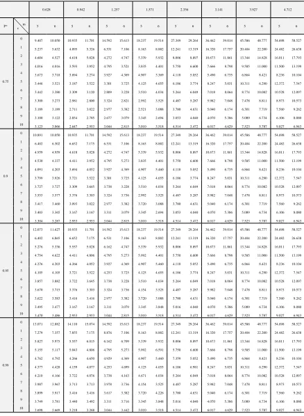
Table 6: Minimum value of the true mean life to specified mean life 𝛍 𝛍⁄ _𝟎for the acceptability of a lot with producer's risk of 0.05 for ASPmed(r, 5, c) and ASPmed(r, 6, c).

0.628 0.942 1.257 1.571 2.356 3.141 3.927 4.712

P* _c m 5 6 5 6 5 6 5 6 5 6 5 6 5 6 5 6

0.75

0 _{9.407 10.050 10.935 11.701 14.592 15.613 18.237 19.514 27.349 29.264 36.462 39.014 45.586 48.777 54.698 58.527} 1 _{5.237 5.632 4.895 5.326 6.531 7.106 8.163 8.882 12.241 13.319 16.320 17.757 20.404 22.200 24.482 26.638} 2 _{4.604 4.527 4.618 5.028 4.272 4.747 5.339 5.932 8.006 8.897 10.673 11.861 13.344 14.828 16.011 17.793} 3 _{4.016 4.016 3.593 3.952 4.795 3.521 3.835 4.401 5.750 6.600 7.666 8.798 9.585 11.000 11.500 13.199} 4 _{3.673 3.718 3.694 3.274 3.927 4.369 4.907 3.369 4.118 5.052 5.490 6.735 6.864 8.421 8.236 10.104} 5 _{3.446 3.521 3.187 3.522 3.301 3.725 4.125 4.655 6.186 3.774 8.247 5.031 10.311 6.290 12.372 7.547} 6 _{3.442 3.380 3.309 3.120 2.809 3.228 3.510 4.034 5.264 6.049 7.018 8.064 8.774 10.082 10.528 12.097} 7

3.300 3.273 2.981 2.800 3.324 2.821 2.992 3.525 4.487 5.287 5.982 7.048 7.478 8.811 8.973 10.573 8 _{3.189 3.189 2.711 3.022 2.977 3.382 2.521 3.088 3.780 4.631 5.040 6.174 6.301 7.719 7.560 9.262} 9 _{3.100 3.122 2.854 2.785 2.677 3.079 3.345 2.694 3.053 4.040 4.070 5.386 5.089 6.734 6.106 8.080} 10 _{3.123 3.066 2.647 2.953 3.044 2.815 3.010 3.518 4.514 3.472 6.017 4.629 7.523 5.787 9.027 6.943}

0.9 0

10.891 10.050 10.935 11.701 14.592 15.613 18.237 19.514 27.349 29.264 36.462 39.014 45.586 48.777 54.698 58.527 1 _{6.402 6.302 6.652 7.175 6.531 7.106 8.163 8.882 12.241 13.319 16.320 17.757 20.404 22.200 24.482 26.638} 2

4.959 4.959 4.618 5.028 4.272 4.747 5.339 5.932 8.006 8.897 10.673 11.861 13.344 14.828 16.011 17.793 3 _{4.530 4.337 4.411 3.952 4.795 5.273 3.835 4.401 5.750 6.600 7.666 8.798 9.585 11.000 11.500 13.199} 4 _{4.091 4.203 3.694 4.052 3.927 4.369 4.907 5.460 4.118 5.052 5.490 6.735 6.864 8.421 8.236 10.104} 5 _{3.799 3.926 3.721 3.522 3.301 3.725 4.125 4.655 6.186 3.774 8.247 5.031 10.311 6.290 12.372 7.547} 6

3.727 3.727 3.309 3.645 3.738 3.228 3.510 4.034 5.264 6.049 7.018 8.064 8.774 10.082 10.528 12.097 7 _{3.553 3.577 3.376 3.303 3.324 3.736 2.992 3.525 4.487 5.287 5.982 7.048 7.478 8.811 8.973 10.573} 8 _{3.417 3.460 3.093 3.022 2.977 3.382 3.720 3.088 3.780 4.631 5.040 6.174 6.301 7.719 7.560 9.262} 9 _{3.403 3.365 3.167 3.167 3.311 3.079 3.345 2.694 3.053 4.040 4.070 5.386 5.089 6.734 6.106 8.080} 10 _{3.304 3.287 2.953 2.953 3.044 2.815 3.010 3.518 4.514 3.472 6.017 4.629 7.523 5.787 9.027 6.943}

0.95

0 _{12.073 11.627 10.935 11.701 14.592 15.613 18.237 19.514 27.349 29.264 36.462 39.014 45.586 48.777 54.698 58.527} 1 _{6.402 6.865 6.652 7.175 6.531 7.106 8.163 8.882 12.241 13.319 16.320 17.757 20.404 22.200 24.482 26.638} 2 _{5.276 5.336 5.557 5.028 6.162 4.747 5.339 5.932 8.006 8.897 10.673 11.861 13.344 14.828 16.011 17.793} 3 _{4.754 4.622 4.411 4.806 4.795 5.273 5.992 4.401 5.750 6.600 7.666 8.798 9.585 11.000 11.500 13.199} 4

4.276 4.203 4.266 4.052 3.927 4.369 4.907 5.460 4.118 5.052 5.490 6.735 6.864 8.421 8.236 10.104 5 _{4.105 4.105 3.721 3.522 4.253 3.725 4.125 4.655 6.186 3.774 8.247 5.031 10.311 6.290 12.372 7.547} 6

3.857 3.882 3.722 3.645 3.738 3.228 3.510 4.034 5.264 6.049 7.018 8.064 8.774 10.082 10.528 12.097 7 _{3.670 3.715 3.376 3.303 3.324 3.736 4.154 3.525 4.487 5.287 5.982 7.048 7.478 8.811 8.973 10.573} 8

3.622 3.583 3.416 3.416 2.977 3.382 3.720 3.088 3.780 4.631 5.040 6.174 6.301 7.719 7.560 9.262 9 _{3.495 3.477 3.167 3.167 3.311 3.079 3.345 3.848 5.016 4.040 4.070 5.386 5.089 6.734 6.106 8.080} 10

3.470 3.486 2.953 2.953 3.044 2.815 3.010 3.518 4.514 3.472 6.017 4.629 7.523 5.787 9.027 6.943

0.99

0 _{13.071 12.882 14.110 15.074 14.592 15.613 18.237 19.514 27.349 29.264 36.462 39.014 45.586 48.777 54.698 58.527} 1 _{7.279 7.357 7.855 7.175 8.876 7.106 8.163 8.882 12.241 13.319 16.320 17.757 20.404 22.200 24.482 26.638} 2 _{5.827 5.975 5.557 6.015 6.162 6.709 5.339 5.932 8.006 8.897 10.673 11.861 13.344 14.828 16.011 17.793} 3 _{5.155 5.117 5.043 4.806 4.795 5.273 5.992 6.591 5.750 6.600 7.666 8.798 9.585 11.000 11.500 13.199} 4 _{4.762 4.792 4.266 4.650 4.929 4.369 4.907 5.460 7.359 5.052 5.490 6.735 6.864 8.421 8.236 10.104} 5 _{4.377 4.428 4.159 4.077 4.253 4.699 4.125 4.655 6.186 6.981 8.247 5.031 10.311 6.290 12.372 7.547} 6 _{4.210 4.166 3.722 4.076 3.738 4.163 4.671 4.034 5.264 6.049 7.018 8.064 8.774 10.082 10.528 12.097} 7 _{3.987 3.967 3.713 3.713 3.978 3.736 4.154 3.525 4.487 5.287 5.982 7.048 7.478 8.811 8.973 10.573} 8 _{3.899 3.917 3.416 3.416 3.617 3.382 3.720 4.226 3.780 4.631 5.040 6.174 6.301 7.719 7.560 9.262} 9 _{3.749 3.781 3.440 3.492 3.311 3.716 3.345 3.848 5.016 4.040 4.070 5.386 5.089 6.734 6.106 8.080} 10