Solving Polynomial Equations using Modified Super Ostrowski Homotopy Continuation Method

(1)

9

Solving Polynomial Equations using

Modified Super Ostrowski Homotopy

Continuation Method

Hafizudin Mohamad Nor*, Amirah Rahman, Ahmad Izani Md. Ismail, Ahmad Abd. Majid

School of Mathematical Sciences, Universiti Sains Malaysia, 11800 Gelugor, Penang, Malaysia.

*Corresponding email: [email protected]

Abstract

Homotopy continuation methods (HCMs) are now widely used to find the roots of polynomial equations as well as transcendental equations. HCM can be used to solve the divergence problem as well as starting value problem. Obviously, the divergence problem of traditional methods occurs when a method cannot be operated at the beginning of iteration for some points, known as bad initial guesses. Meanwhile, the starting value problem occurs when the initial guess is far away from the exact solutions. The starting value problem has been solved using Super Ostrowski homotopy continuation method for the initial guesses between 1000x₀ 1000 . Nevertheless, Super Ostrowski homotopy continuation method was only used to find out real roots of nonlinear equations. In this paper, we employ the Modified Super Ostrowski-HCM to solve several real life applications which involves polynomial equations by expanding the range of starting values. The results indicate that the Modified Super HCM performs better than the standard Super Ostrowski-HCM. In other words, the complex roots of polynomial equations can be found even the starting value is real with this proposed scheme.

(2)

10

1. INTRODUCTION

Consider a polynomial equation ( ) 0.

f x  (1)

There are four classes of methods to solve such equations - graphical methods, bracketing methods, open methods and global methods. According to Chapra [1], the graphical method can be utilized to obtain rough estimates of roots to use as starting value for other numerical methods. Chapra [1] also stated that the bracketing method (interval method) refers to a method that uses two initial guesses that “bracket” the root, while open methods (local method) do not require the initial guesses bracket the root. Global method, as in Gritton et al. [2], was defined as finding a solution from an arbitrary starting guess. Bisection method and false position method are classified as bracketing methods. Secant method, fixed point method, Newton’s method and Ostrowski’s method are categorized as open methods. An example of a global method is the homotopy continuation method (HCM).

There are two types of mathematical problem when using classical methods in solving polynomial equations - divergence and starting value problems. Newton’s and secant methods contain the derivatives f'( )x or its estimates f b( )f a( ) in the denominator of their respective formulae. According to Chapra and Canale [3], the divergence of classical methods occurs when there is division by zero at initial iterations. The divergence problem associated with Ancient Chinese Algorithms, Newton’s method, Adomian method, Secant method and Ostrowski’s method were successfully solved in Wu’s works [4 – 7] and Nor et al. [8] respectively. Ku et al. [9] stated that Newton’s method can often converge remarkably quickly (quadratic convergence) if the starting value is sufficiently close to the roots. In other words, Newton’s method will face the starting value problem when the starting value is far away from the exact solutions. There are only a few works in solving the starting value problem, which include Gritton et al. [2] dan Nor et al. [10]. In this paper, we improve the method of Nor et al. [10] by introducing a better scheme known as Modified Super Ostrowski-HCM.

2. SUPER OSTROWSKI-HCM AND ITS STARTING VALUE PROBLEM

The method of Super Ostrowski-HCM was developed as in Nor et al. [10]. Super Ostrowski-HCM was developed by combining Ostrowski-HCM with a new homotopy and a new auxiliary homotopy functions that were introduced by Nor et al. [11, 12] respectively. To illustrate the issues associated with the method, we consider the following example.

Example 2.1. Consider the following quadratic equations in Rahimian et al. [13] 2

( ) 4 13 0

f x x  x  (2)

The number of roots for (2) is no more than d 2. The exact solutions are located in the complex domain that is x₁ 2 3i and x₂  2 3i. The familiar way to find the location of roots is by computing 2

4

(3)

11

that there are no real solutions to be found. In other words, all roots are in the complex domain. The results are shown as in Table 1.

Table 1: The Problem of Super Ostrowski-HCM for (2)

Starting Value x₀ Approximate Solution x_k Number of Iteration

0 Indeterminate Indeterminate

100

 Indeterminate Indeterminate

100 Indeterminate Indeterminate

100 i

  x₁ 2 3i 4

100i x2  2 3i 7

Table 1 shows that the approximate solution cannot be found using Super Ostrowski-HCM when the starting values are real. However, the approximate solution can be found when the starting values are complex numbers.

The question arises, how to determine the proper starting values when the user does not know the types of roots especially when there is increment in the order of polynomial function. The difficulty in determining the location of roots can cause the difficulty to determine the starting values. Therefore, we investigate the problem and we provide the solution to the problem.

3.0 DEVELOPMENT OF MODIFIED SUPER OSTROWSKI-HCM

The disadvantage of Super Ostrowski-HCM was shown in the previous section. We now modify the scheme in [10] by modifying Quadratic Bezier homotopy function (QBHF) and linear fixed point function (LFPF). We modify QBHF and LFPF to the Quadratic Parameter homotopy function (QPHF) and Quadratic Parameter Fixed Point (QPFP) function. However, we still use Ostrowski-HCM as our basis method.

3.1 Ostrowski-HCM

Ostrowski’s method was pioneered by Alexander Markowich Ostrowski [14,15]. Then, Ostrowski’s method was widely used for the development of other formulae such as the formula introduced by Kou et al. [16], Grau and Diaz-Barrero [17], Sharma and Guha [18] and Chun and Ham [19]. The formula for Ostrowski’s method is as follows:

1

( ) , '( )

( ) ( )

, ( ) 2 ( ) '( )

i

i i

i

i i

i i i

f x

y x

f x

f x f y

x y

f x f y f x



 



i0,1, 2,...,k1. (3)

(4)

12 1 ( , ) , ( , ) ( , ) ( , ) , ( , ) 2 ( , ) ( , )

i

i i

x i

i i

i i x i

H x t

y x

D H x t

H x t H y t

x y

H x t H y t D H x t



 



0,1, 2,..., 1,

i k (4)

where H x t( , ) is homotopy function and D H x t_x ( , ) is the derivative of the homotopy function with respect to x. The convergence of Ostrowski-HCM was stated in Nor et

al. [10] as linear.

3.2 Quadratic Parameter Homotopy Function

Verschelde et al. [20] used the following homotopy function

( , ) (1 )k ( ) k ( ),

H x t  t G x t F x   (5)

where x{ ,x x1 2,...,xn}, ( ) ( 1( ), 2( ),..., ( ))

T n

G x  g x g x g x and F x( )( ( ),f x₁ f₂( ),...,x f_n( ))x T to solve a sparse polynomial system. Since we are now dealing the solution of single equation and second degree of parameter t, therefore the homotopy function (5) can be

reduced to

2 2

( , ) (1 ) ( ) ( ),

H x t  t g x t f x  , (6)

when k2 and n1. Nor et al. [21] introduced a new homotopy function and then named this function as Quadratic Bezier homotopy function in Nor et al. [11]. Quadratic Bezier homotopy function was developed from a widely used homotopy function. The standard homotopy function H x t( , ) as in Gritton et al. [2], Rahimian et

al. [13], Jalali-Farahani and Seader [22] and a collection of Wu’s works [4 – 7] can be written as follows

( , ) (1 ) ( ) ( ),

H x t  t g x tf x t[0,1], (7)

where g x( ) is an auxiliary homotopy function (starting function) and f x( ) is the target

function. Both homotopy functions (5) and (7) will be equal when the value of  1

and k1. The standard homotopy function (7) satisfies two boundary conditions at two endpoints which implies

( , 0) ( ), ( ,1) ( ).

H x g x

H x f x



 (8)

Since we are now dealing with the solution of polynomial equations f x( )0, so that ( , ) 0,

H x t  t[0,1]. (9)

We now modify the Quadratic Bezier homotopy function

2 2

2( , ) (1 ) ( ) 2 (1 ) ( , ) ( ),

H x t  t g x  t t H x t t f x (10)

and homotopy function (6) to

* 2 2

2( , ) (1 ) ( ) (2 ) ( ), !

H x t t g x t t f x

d



    (11)

where  is a complex constant and d is the highest degree of polynomial equations. Function (11) is obtained from

* 2 2

2( , ) (1 ) ( ) (1 (1 ) ) ( )

! .

H x t t g x t f x

d



(5)

13

The complement of parameter (1t)2 is 1 (1 t)2. Therefore, we make (2tt2) as the coefficient of the target function f x( ). By eliminating the middle term of QBHF, the

function obtained (11) looks simpler than the function before. Mathematically, the equation (10) and (11) can be expressed respectively using matrix representation



2



2

1 2 1 ( ) ( , ) 1 2 2 0 ( , ) ,

1 0 0 ( )

g x

H x t t t H x t

f x                (13) to





* 2 2

0 1 ( ) ( , ) 1 2 0 2 ( , ) ,

0 0 ( )

g x

H x t t t H x t

f x                   (14) where ! d 

  . All of eq. (6), (10) and (11) fulfill the following two boundary

conditions at two endpoints which implies *

2 2

( , 0) ( , 0) ( , 0) ( ) 0,

H x H x H x g x  (15)

*

2 2

( ,1) ( ,1) ( ,1) ( ) 0,

H x H x H x  f x  (16)

when t0 and t 1 respectively.

3.3 Quadratic Parameter Fixed Point Function

A factor which contributes to accuracy improvement is the auxiliary homotopy function

( )

g x or the starting function when t0 at the point xx₀ [10]. The auxiliary homotopy functions that are in common use are Newton function, fixed-point function and affine function are discussed in [2, 13, 22]. The best auxiliary homotopy function is the following fixed point function as stated in Nor et al. [12]:

0

( ) .

g x  x x (17)

Nor et al. [12] improved upon the fixed point function (17) by introducing the following function

0

( , ) (1 )( ) ( ).

g x t  t xx tf x (18)

named as Linear Fixed Point (LFP) function. Nor et al. [10] stated that the advantage LFP has over the standard fixed point function is that g x t( , ) always moves for every

increment in parameter t

0

( , 0) ( ),

( , 0 1) (1 )( ) ( ), ( ,1) ( ).

g x x x

g x t t x x tf x

g x f x

 

     



(19)

We are now improving the order of LFP to second order such that

* 2

2 0

2 ( , ) (1 ) ( ) (2 ) ( ),

!

g x t t x x t t f x

d



     (20)

where  is a complex constant, d is the highest degree of polynomial equationsand t

is a loading parameter t[0,1]. We believe that the increase in order will increase the

(6)

14 3.4 Modified Super Ostrowski-HCM

As the Super Ostrowski-HCM was developed by combining Ostrowski-HCM with Quadratic Bezier homotopy function and Linear Fixed Point Function, the Modified Super Ostrowski-HCM also is developed with the same technique. The Super Ostrowski-HCM is then improved to Modified Super Ostrowski-HCM by combining Ostrowski-HCM with Quadratic Parameter homotopy function and Quadratic Parameter Fixed Point Function. The method put forward is

*

2 1

*

2 1

* *

2 1 2 1

1 * * *

2 1 2 1 2 1

( , ) , ( , )

( , ) ( , ) , ( , ) 2 ( , ) ( , )

i i

x i i

i i i i

i i

i i i i x i i

H x t

y x

D H x t

H x t H y t

x y

H x t H y t D H x t

             (21)

where the homotopy function H*₂( , )x t in (11) is improved to

* 2 * 2

2( , ) (1 ) 2( , ) (2 ) ( )

H x t  t g x t  tt f x where

!

d



  and the starting function g*₂( , )x t is as

per (20). To limit the scope of complex constant , we set   [ 1 i,1i]. We solve *

2( ,i i 1) 0

H x t_  by iterating model (21) twice for every t_i_₁ to find x_i_₁.We re-solve Example 2.1 using the Modified Super Ostrowski-HCM. The results are shown as follows

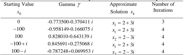
Table 2: The Solution for Super Ostrowski-HCM for Eq. (2)

Starting Value

0

x

Gamma  Approximate Solution x_k

Number of Iterations

0 -0.773500-0.370411 i

1 2 3

x   i 3

100

 -0.958149-0.166075 i

1 2 3

x   i 4

100 0.828010-0.643139 i

2 2 3

x   i 4

100 i

  0.845691+0.275068 i

1 2 3

x   i 4

100i -0.787248+0.069953 i

2 2 3

x   i 4

Table 2 provides results that show a marked improvement over those reported in Table 1. Our proposed method can converge quickly to the any solution of polynomial equations. In other words, the proposed method can track the complex roots even when the starting values are real with the fewer iterations.

4. NUMERICAL EXPERIMENTS AND DISCUSSION

We test four examples of applications involving polynomial equations. The Modified Super Ostrowski-HCM is demonstrated using several starting values which are automatically generated within a specified interval. The value of  is also randomly generated in the interval of     1 i  1 i and the stopping criterion used is

( ) ,

f x  (22)

(7)

15

Example 4.1. Consider the following azeotropic-point calculation discussed in Gritton et al. [2]

2

( ) 6.5886408 4.0777367 0,

f x x  x  (23)

where the exact solutions are x10.691473843274813 and x25.89716695672519. The results are shown in Table 3 by varying the values of starting value which are randomly selected from the interval 6 6

0

10 x 10

   .

Table 3: Demonstration of Modified Super Ostrowski-HCM for Eq. (23)

Starting

Value x₀ Gamma 

Number of

iterations x f x( )

89636

 -0.029444+0.656554 i 6 0.69147384326713523528 4.00×10-11

321381 -0.894890+0.793899 i 12 5.8971669567278777180 1.40×10-11

Table 3 shows that:

i. The Modified Super Ostrowski-HCM perform efficiently even though the starting value is very large.

ii. The Modified Super Ostrowski-HCM can track all isolated solutions even when it is located in the complex domain.

iii. The number of iterations is less than 20 even though the starting value is very far from the exact solutions.

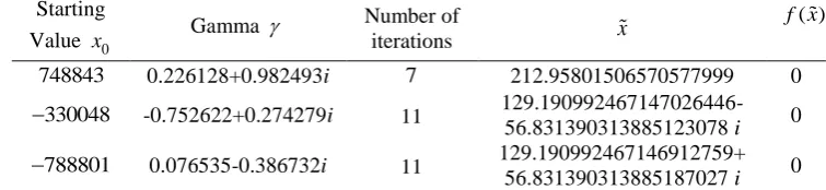
Example 4.2. Consider the following scalar of polynomial equations in Gritton et al. [2] which relates to the calculation of the specific volume of a gas using virial equation of state:

3 2

( ) 471.34 74944.6341 4242149.1 0,

f x x  x  x  (24)

where the exact solutions are x₁212.95801506571 and one pair of complex roots

2, 3 129.190992467147 56.831390313885 i.

x x   The results are shown in Table 4 by

varying the values of starting value which are randomly selected from the interval

6 6

0

10 x 10

   .

Starting

Number of

iterations x

( )

f x

748843 0.226128+0.982493i 7 212.95801506570577999 0

330048

 -0.752622+0.274279i 11 129.190992467147026446-56.831390313885123078 i 0

788801

 0.076535-0.386732i 11 129.190992467146912759+ _{56.831390313885187027}_i 0

Table 4 shows that:

(8)

16

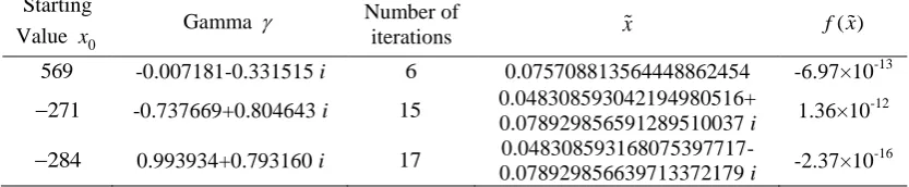
Example 4.3. Consider the following scalar of polynomial equations in Gritton et al. [2] which relates to the calculation of a gas using Redlich-Kwong equation of state:

3 2

( ) 0.172326 0.015878415 0.00064834321 0,

f x x  x  x  (25)

where the exact solutions are x₁0.0757088136642496 and one pair of complex conjugates x₂,x₃0.0483085931678752 0.0789298566391914 i. The results are shown in Table 5 by varying the values of starting value which are randomly chosen from the interval 1000x₀ 1000.

Starting

Number of

iterations x f x( )

569 -0.007181-0.331515 i 6 0.075708813564448862454 -6.97×10-13

271

 -0.737669+0.804643 i 15 0.048308593042194980516+

0.078929856591289510037 i 1.36×10

-12

284

 0.993934+0.793160 i 17

0.048308593168075397717-0.078929856639713372179 i -2.37×10

-16

Table 5 shows that:

iii. The numbers of iteration is less than 20 even though the starting value very far from the exact solutions.

Example 4.4. Consider the following fourth-order of polynomial equations in Gritton et al. [2] associated with a chemical equilibrium problem:

4 3 2

( ) 1.3 0.699096 0.1816915 0.00850239 0.

f x x  x  x  x  (26)

The number solutions of Eq. (26) should be no more than d4. The exact solutions are x₁ 0.0586545664906674, x₂ 0.600323276889981and one pair of complex conjugates

3, 4 0.320511078309676 0.372474896861919 i

x x   . The results are shown in Table 6 by

varying the values of starting value which are randomly chosen from the interval

6 6

0 10 x 10 .

  

Starting

Value x₀

Gamma Number of

iterations

x f x( )

950853

 0.223712+0.534741i 14 0.058654566499061970564 -9.43×10-13

314443 -0.807889-0.546452i 14 0.60032327753233616363 7.55×10-11

515748

 0.879757-0.111409i 26 0.32051107830967612289+

0.37247489686191936897 i -1.39×10

(9)

17

529268 -0.076049+0.831413i 18

0.32051107864183076002-0.37247489729603061592 i 7.02×10

-11

Table 6 shows that:

5. CONCLUSION

Table 1 indicates the drawback of Super Ostrowski-HCM when solving a quadratic equation with no real roots. Table 2 provides the solution for Super Ostrowski-HCM by upgrading its formula. The results from Tables 3 – 6 indicate the effectiveness and efficiencies of Super Ostrowski-HCM after modifications are made to it. The effectiveness and efficiencies of proposed method are measured with the ability of method to track the complex roots and the ability of method to converge to the exact solution with fewer iterations. The Modified Super Ostrowski-HCM performs well even when the user does not have the sufficient knowledge about the characteristics of roots.

ACKNOWLEDGMENTS

Part of this research has been supported by a grant of USM RUI grant 1001/PMATHS/811252 and a scholarship MyBrain15-MyPhD from Kementerian Pengajian Tinggi Malaysia. The authors would like to thank the anonymous reviewers whose constructive comments were helpful in improving the quality of this paper.

REFERENCES

[1] Chapra, S. C. (2012). Applied Numerical Methods with MATLAB for Engineers and Scientist, 3rd Edition, McGraw-Hill, New York, USA.

[2] Gritton, K. S., Seader, J. D. and Lin, W. (2001) “Global homotopy

continuation procedures for seeking all roots of a nonlinear equation”,

Computers and Chemical Engineering, Vol. 25, pp 1003 – 1019.

(10)

18

[4] Wu, T. M. (2005). “A modified formula of ancient Chinese algorithm by the homotopy continuation technique”, Applied Mathematics and Computation, Vol. 165, pp 31-35.

[5] Wu, T.M. (2005), “A study of convergence on the Newton-Homotopy continuation method”, Applied Mathematics and Computation 168 , pp. 1169-1174.

[6] Wu, T.M. (2006), “A new formula of solving nonlinear equations by Adomian and homotopy methods”, Applied Mathematics and Computation 172 , pp. 903-907.

[7] Wu, T.M. (2007), “The secant-homotopy continuation method”, Chaos Solitons and Fractals 32, pp. 888-892.

[8] Nor, H. M., Rahman, A., Md. Ismail, A. I., and Majid, A. A. (2014), “Numerical solution of polynomial equations using Ostrowski homotopy continuation method”, MATEMATIKA, Vol.30 (1), pp. 47 – 57.

[9] Ku, C., Yeih W. and Liu C. (2010). “Solving non-linear algebraic equations by a scalar Newton-homotopy continuation method” International Journal of Nonlinear Sciences & Numerical Simulation. Vol. 11(6), pp. 435 – 450.

[10] Nor, H. M, Rahman, A., Md Ismail, A. I. & Majid, A. A. (2014). “Superior accuracy of Ostrowski homotopy continuation method with quadratic Bezier homotopy and linear fixed point functions for nonlinear equations” in International Conference on Quantitative Sciences and Its Applications 2014, AIP Conference Proceedings 1635, American Institute of Physics, Melville, NY, pp. 174-181.

[11] Nor, H. M., Md. Ismail, A. I., and Majid, A. A. (2014). “Quadratic Bezier homotopy function for solving system of polynomial equations,

MATEMATIKA, Vol.29 (2), pp. 159 – 171.

[12] Nor, H. M, Md Ismail, A. I. & Majid, A. A. (2014) “Linear fixed point function for solving system of polynomial equations” in The 3rd International Conference on Mathematical Sciences, AIP Conference Proceedings 1602, American Institute of Physics, Melville, NY, pp. 105 – 112.

[13] Rahimian, S. K., Jalali, F., Seader, J. D. and White, R. E. (2010). “A new homotopy for seeking all real roots of a nonlinear equation”, Computers and Chemical Engineering. Vol. 35, pp. 403 - 411.

(11)

19

[15] M. Ostrowski (1973). Solution of Equations in Euclidean and Banach Space, 3rd Edition. Academic Press, New York.

[16] Kou, J., Li, Y. and Wang, X. (2007). “Some variants of Ostrowski’s method with seventh-order convergence”, Journal of Computational and Applied Mathematics. Vol. 209, pp. 153 – 159.

[17] Grau, M. and Diaz-Barrero, J. L. (2006). “An improvement to Ostrowski root-finding method”, Applied Mathematics and Computation, Vol. 173, pp. 450 – 456.

[18] Sharma, J. R. and Guha, R. K. (2007). “A family of Modified Ostrowski methods with accelerated sixth order convergence”, Applied Mathematics and Computation. Vol. 190, pp. 111 – 115.

[19] Chun, C. and Ham, Y. (2007). “Some sixth-order variants of Ostrowski root-finding methods”. Applied Mathematics and Computation, Vol. 193, pp. 389 – 394.

[20] Verschelde, J. (1996), Homotopy continuation methods for solving polynomial systems, PhD Thesis, Katholieke Universiteit Leuven, Belgium.

[21] Nor, H. M, Md Ismail, A. I. & Majid, A. A. (2013), “A new homotopy function for solving nonlinear equations” in International Conference on Mathematical Sciences and Statistics 2013, AIP Conference Proceedings 1557, American Institute of Physics, Melville, NY, pp. 21-25.

(12)