67
This open access article is distributed under a Creative Commons Attribution (CC-BY SA) 3.0 license
SERIES SOLUTION OF TYPHOID FEVER MODEL USING
DIFFERENTIAL TRANSFORM METHOD
O. J. Peter1*, O. B. Akinduko2, C. Y. Ishola 3, O. A. Afolabi 4, A. B. Ganiyu5
1,4,5 Department of Mathematics, University of Ilorin, Ilorin, Kwara State, Nigeria. 2Department of Mathematical Sciences, Adekunle Ajasin University Akungba,Ondo State.
4Department of Mathematics, National Open University of Nigeria Jabi, Abuja Nigeria 1[email protected], 2[email protected], 3[email protected], 4
[email protected] , [email protected] *Corresponding author: [email protected] +2348033560280
ABSTRACT
This paper presents an analysis of PSIuIeTR type model, which are used to study the transmission dynamics of typhoid fever diseases in a population. Basic idea of typhoid fever disease transmission using compartmental modeling is discussed. Differential Transformation Method (DTM) is discussed in detail, which is used to compute the series solution of the non-linear system of differential equation governing the model equations. The validity of the (DTM) in solving the proposed model is established by classical fourth-order Runge-Kutta method which is implemented in Maple 18. Graphical results confirm that (DTM) is in good agreement with RK-4 and this produced correctly same behaviour of the model, thus validating the efficiency and accuracy of (DTM) in finding the series solution of an epidemic model.
Keywords: Typhoid Fever , Differential Transform Method, Runge-Kutta Method.
1. Introduction
Typhoid fever, a communicable disease which infects human only and occurs due to systemic infection mainly by salmonella typhi organism that causes symptoms. It is an acute generalized infectious disease of the intestinal lymphoid tissue and the gall bladder. Incubation period of typhoid fever, usually 10-14 days but it may be as short as 3 days or as long as 21 days. The disease is transmitted from person-to-person as a result of improper hygiene and unsafe food and water handling practices. Recent report, however, suggests that individuals may be indirectly infected with typhoid through contact with fecal and urine contamination in their immediate environment. (Shanahan, 1998).
The disease is endemic in many developing countries where water supply sanitation and waste treatment is inadequate. The disease remains a substantial public health problem. Globally, the disease burden was estimated to be over 16 million cases of illness each year, resulting in over 600,000 mortality rates Mushayabasa (2011).
68
This work focused on the application of differential transform method to the proposed model and to verify the validity of the method in solving the model equations using computer in-built Maple 18 classical fourth-order Runge-Kutta method as a base. In recent years, the differential transform method (DTM) is mostly used for solving non-linear ordinary and partial differential equations. It is a semi-analytic technique that formalizes the Taylor series in a totally different approach. The concept of (DTM) was first introduced by Zhou, (1986) in a study to solve nonlinear problems of electrical circuits. The DTM obtains an analytical solution in form of polynomial. DTM has been successfully applied to solve many nonlinear problems arising in engineering, mathematics, physics and mechanics. Abazari et al, (2010). The main advantage of DTM is that it can be applied directly to solve linear and nonlinear Ordinary Differential Equations without requiring linearization, discretization or perturbation. (Hassan, 2008; Peter & Ibrahim, 2017; Akinboro, et al 2014).
We employ the (DTM) to the system of differential equations which describe the proposed model and approximate the solutions in a sequence of time intervals. In other to verify the accuracy and validity of the (DTM), we compared the obtained results with fourth-order Runge-Kutta Method.
2. Methodology
This section describes the formulation of the model. The human populations N(t) is divided into six sub-populations namely; protected class, P(t), susceptible class, S(t), uneducated infectious class, Iu(t), educated infectious class Ie(t), treated class T(t) and recovered individuals class,
) (t
R . Individuals are recruited into the susceptible class by either immigration or birth at the rate
. Susceptible individuals acquire typhoid infection at per capita rate
. We assume that proportion
progress to educated infectious class, while the compliment1
progress to uneducated infectious compartment class. Susceptible individuals received vaccination to protect themselves against the disease at the rate
. Since vaccine wanes with time, then after its expiry, the protected individuals return back to susceptible class at the rate
. We assume that individuals in each compartment undergo a natural death at the rate . Let
1,
2, and
3 be transmission69
Figure 1. Pictorial Representation of Model
2.1 Model Assumptions
1. Recovered individuals may become susceptible again at the rate
, this is due to the fact that typhoid does not confer permanent immunity on recovery.2. Susceptible individuals receive vaccination to protect themselves against infection at the rate
.3. Susceptible individual can be infected through a direct contact with educated infected or uneducated infected.
4. All parameters are non-negative.
5. No treatment failure. All treated individuals recoverd.
R T dt
dR
T I
I dt
dT
Iu I S
dt dIe
I S
dt dIu
S P
S dt
dS
P S
dt dP
e u
e
u
=
) (
=
) (
=
) (
) (1 =
) ( =
) ( =
3 2
1
2 2
1 1
(1)
70
T
I
I
u 2 e 3 1=
(2)Substituting the value of force of infection
R T dt dR T I I dt dT I I T I I S dt dIe I S T I I dt dIu S P S T I I dt dS S P S dt dP e u u e e u u e u e u
= ) ( = ) ( ) ( = ) ( ) )( (1 = ) ( ) ( = ) ( = 3 2 1 2 2 3 2 1 1 1 3 2 1 3 2 1 (3)Table 1. Description of Variables and Parameters for the Model
Variables Description
) (t
P protected individuals at time t
) (t
S susceptible individuals at time t
Iu
uneducated infectious individuals at time tIe
educated infectious individuals at time t tT treated individuals at time t t
) (t
R recovered individuals at time t
Parameters Interpretation
recruitment rate of susceptible individuals
natural death rate
1
disease induced death rate for Iu class2
disease induced death rate forIe3
disease induced death rate for T1
treatment rate for Iu2
treatment rate for Ie
wanning rate of vaccine
rate of recovery from treatment rate of educating or counseling uneducated infectives
rate of vaccinating individual in the susceptible class1
transmission rate betweenS
and Iu class2
transmission rate betweenS
and Ie class3
71 2.2 Existence and Uniqueness of Solution
The implementation of any mathematical model largely based on whether the given system of equations has a solution, and if the solution is unique, we shall use the Lipchitz condition to verify the existence and uniqueness of solution for the system of the model equation 3.
Let the system of equations of the model be as follows:
R
T
A
I
I
A
I
I
T
I
I
S
A
I
S
T
I
I
A
S
P
S
T
I
I
A
P
S
A
e u u e e u u e u e u
=
)
(
=
)
(
)
(
=
)
(
)
)(
(1
=
)
(
)
(
=
)
(
=
6 3 2 1 5 2 2 3 2 1 4 1 1 3 2 1 3 3 2 1 2 1Theorem 1. (Derrick and Groosman,1976)
Let B denote the region
) ,... , ( = ), ..., , ( = 1,
, 0 1 2 10 20
0 b x x x x x xn xo x x xno t
t
And suppose that a(t,x) satisfies the Lipchitz condition
2 1 2
1) ( , )
,
(t x a t x k x x
a
whenever the pairs (t,x1) and (t,x2) belong to B where
k
is a positive constant. Then, there is aconstant
0
such that there exists a unique continuous vector solution of x(t) of the system in the intervalt
t
o
. It is important to note that the condition is satisfied by the requirement that, 1,2,3 = ,
,i j
x a j i
be continuous and bounded in B Considering the model equation 3 , we are
interested in the region
0
R
.
. We look for the bounded solution in the region and whose partialderivatives satisfy a
0. where
and
are positive constants.Theorem 2
Let B denote the region
0
R
, then equation 3 have a unique solution. We show that6
,
1,2,3,4,5
=
,
,
i
j
x
a
j i
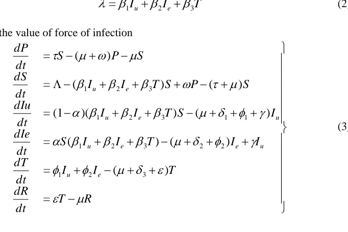
Are continuous and bounded in B For A1 < ) ( =
1
72
For A2
< = 2
P a < ) ( ) (= 1 2 3
2
T e
u I I
I S a
<
=
1 2S
I
a
u
,
<
=
2 2S
I
a
e
, < = 3 2 S T a
< 0 = 2 R a ,For
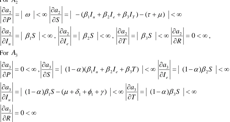
A
3 < 0 = 3 P a , < ) )( (1
= 1 2 3
3 T I I S a e
u
<
)
(1
=
2 3S
I
a
e
<
)
(
)
(1
=
1 1 13
S
I
a
u < ) (1 = 3 3 S Ta
< 0 = 3 R a
These partial derivative exist, continuous and are bounded, similarly for A4 through to
A
6 . Hence, by theorem 2, the model has a unique solution3. Result and Analysis
The processes involved in DTM is given as follows: Given an arbitrary function of
x
, suppose )(x
e is a non-linear funtion of
x
, then e(x) can be expanded in a Taylor series about a pointx
=0
as0 = 0 = ) ( ! 1 = ) ( x k k k k x e dx d k x x e
Thus,the differential Transform of y(x) is given as:
0 = ) ( ! 1 = ) ( x k k x e dx d k k E
and the inverse differential Transform is given as
k k
x
k
E
x
e
(
)
=
(
)
0 =
73
Table 2. Basic operation properties of the DTM
S/No Original Function Transformed Function
1 e(x)=m(x)n(x) E(k)=M(k)N(k)
2 e(x)=m(x) E(k)=M(k),
is a constant3
dx
x
dm
x
e
(
)
=
(
)
E(k)=(k1)M(k1)4 2 2
)
(
=
)
(
dx
x
c
d
x
e
2) ( 2) 1)( ( = )(k k k C k
E
5
a adx
x
m
d
x
e
(
)
=
(
)
E(k)=(k1)(k2) (k n)C(kn)6
e(x)=1 E(k)=(k)7
e(x)=x E(k)=(k 1),
is the Kronecker delta8
( )=
)
(
x
e
xe
!
=
)
(
k
k
E
k
9
e(x)=c(x)d(x) ( )= ( ) ( )0
=D a C k a
k
E k
n
10
ax
x
e
(
)
=
(1
)
!
1)
(
2)
1)(
(
=
)
(
k
k
a
a
a
a
k
E
3.1 Solution of the Model
In this section, we apply the steps involved in differential transform method as follows: Using the operational properties (1), (2), (6) and (7) in Table 2 and applying them to the systyem of differential equations in (1) we obtain the following system of transformed equations below,
where
1
3 3
4 3
1
2 5 3
1
2
=
,
K
=
,
K
=
,
K
=
,
K
=
K
]
[
1
1
=
1)
(
S
k
K
1P
k
k
k
P
,0
][ 1 1 = 1)
( 1 2 3 2
0 = k S K l k T l k I l k I l S k P k b k k
S u e
k l
1
][ 1 1 = 1)
( 1 2 3 3
0 = k I K l k T l k I l k I l S k k
I u e u
k
l
u
] [ 1 1 = 1)( 1 2 3 4
0 = k I K k I l k T l k I l k I l S k k
I u e u e
k
l
e
74
]
[
1
1
=
1)
(
1I
k
2I
k
K
5T
k
k
k
T
u
e
]
[
1
1
=
1)
(
T
k
R
k
k
k
R
Subject to the following initial conditions P(0)=100, S(0)=200,
I
u(0)
=
140
,I
e(0)
=
120
,80 = (0)
T , R(0)=60. Using the initial conditions and the parameter values in the table we have the following series solutions.
when
k
=
5
the solution to the system (3) in closed form is obtained as3 2 0 = 3 56687.7415 0 2175.73180 44.200 100 = ) ( = )
(t P k t t t t
P k k n
7 4 9 5
10 * 3 1.46744524 10 * 8
2.27893997 t t
3 8 2 6 0 = 10 * 0 9.11212056 10 * 4 1.71460044 43798.400 200 = ) ( = )
(t S k t t t t
S k k n
10 4 13 5
10 * 8 2.18028835 10 * 8
7.35185700 t t
3 8 2 6 0 = 10 * 7 9.04955022 10 * 4 1.69046847 43573.7200 140 = ) ( = )
(t Iu k t t t t
Iu k k n
10 4 13 5
10 * 0 2.16537688 10 *
7.2867056 t t
3 6 2 0 = 10 * 3 6.22601159 4 25367.7473 338.7600 120 = ) ( = )
(t I k t t t t
Ie k k n
8 4 5 5
10 * 5 1.48279838 10 * 0
6.64669221 t t
3 2 0 = 5 24886.1780 0 924.682360 7.760 80 = ) ( = )
(t T k t t t t
T k k n
6 4 8 5
10 * 0 6.21641792 10 * 0
9.52033979 t t
3 2 0 = 1 123.443351 1. 23.480 60 = ) ( = )
(t R k t t t t
R k k n
5 5
4 10 * 4 7.61697735 6
2484.23556 t t
4. Numerical Simulation and Graphical Illustration of the Model.
75
Table 3. Parameters values for the model
Parameter Initial Value Source
200
Assumed
0.142
Mushayabasa, (2011)
0.4
Kariuki, C. (2011)
0.6
Assumed
0.5
Assumed
0.1
Estimated
0.0072
Assumed1
1.5
Kalajdzievska, D. (2011),2
0.05
Assumed3
0.05
Assumed
0.075
Lawi, (2011)1
0.04
Estimated2
0.3
Estimated76
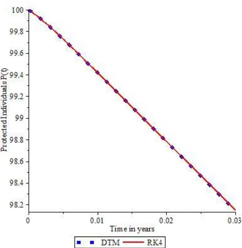
Figure 3. Solution of Susceptible Population by DTM and RK4
77
Figure 5. Solution of Educated Infected Population by DTM and RK4
78
Figure 7. Solution of Recovered Population by DTM and RK4
4.1 Discussion of Results
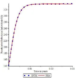
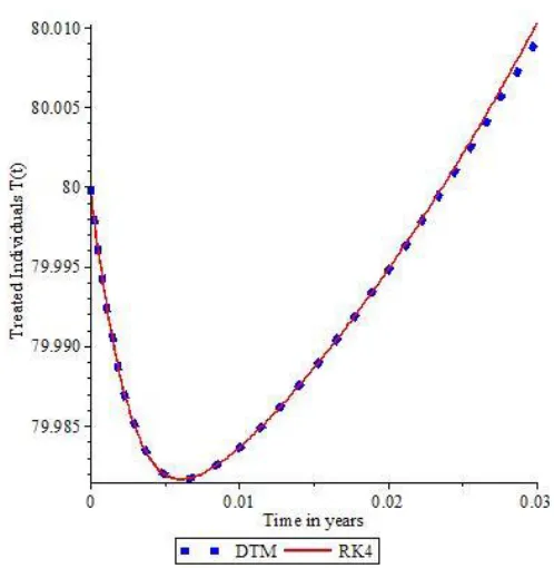
The solutions obtained by using Differential Transform Method with given initial conditions compared favourably with the solution obtained by using classical fouth-other Runge-Kuta method. The solutions of the two methods follows the same pattern and behaviour. This shows that Differential Transform Method is suitable and efficient to conduct the analysis of epidemic models.
5. Conclusion
79 References
Abazari, R., & Borhanifar, A. (2010). Numerical study of the solution of Burgers’ and coupled Burgers’ equations by differential transformation method. Comput. Math Appl.59, 2711– 2722.
Adetunde, I. A. (2008). Mathematical models for the dynamics of typhoid fever in kassena-nankana district of upper east region of Ghana. J. Modern Math Stat, 2, 45-49.
Akinboro, F. S., Alao, S., & Akinpelu, F. O. (2014). Numerical solution of SIR model using differential transformation method and variational iteration method. General Mathematics Notes, 22 (2), 82-92.
Chamuchi, M. N., Johanna K. S, Jeconiah, A. O & James, M.O (2014). SIIcR model and simulation of effects of carriers on transmission dynamics of Typhoid fever in KI’isii Town Kenya, SIJ (CSEA), 2(3), 109 - 116 .
Cvjetanovic, B., Grab, B., Uemura, K. (2014). Epidemiological model of typhoid fever and its use in the planning and evaluation of antityphoid immunization and sanitation programmes,
Bull. Org. Mond. Sante (45),53-75.
Derrick, N. R & Grossman, S. L (1976). Differential Equation with application. Addision Wesley Publishing Company, Inc. Philippines.
Hassan, I. H.(2008).Application of Differential Transform Method for solving systems of Differential Equations. Applied Math Modeling. 32, 2552-255.
Hyman, J. M. (2006). Differential Susceptibility and Infectivity Epidemic Models", Math.Biosci. Eng., 3, 88-100.
Joshua, E.. (2011). Mathematical model of the spread of Typhoid fever. World Journal of Applied Science and Technology, 3(2), 10-12.
Kalajdzievska, D. “Modeling the Effects of Carriers on the Transmission Dynamics of Infectious Diseases”. Math Biosci Eng, 8(3), 711–722
Kariuki, C. (2011). Characterization of Multidrug-Resistant Typhoid Outbreaks in Kenya.
J.C.Micbol, 42(4), 1477-1482.
Lauria, D. T., Maskery, T., Poulos, C.,Whittington, D. (2009). An optimization model for reducing typhoid cases in developing countries without increasing public spending, Vaccine, JVAC-8805 http://dx.doi.org/10.1016/j.vaccine.2008.12.032
Moatlhodl, K.& Gosaamang, K. R. (2017). Mathematical Analysis of Typhoid Infection with Treatment. Journal of Mathematical Sciences: Advances and Applications, 40, 75-91. Muhammad, A. K., Muhammad, P. I., Saeed, K.. Ilyas, S. Sharidan, G. & Taza, M.(2015).
Mathematical Analysis of Typhoid Model with Saturated Incidence Rate. Advanced Studies in Biology, 7( 2), 65 - 78.
80 and Statistics, 5(2), 54-59.
Nthiiri, J. K.., Lawi, G. O., Akinyi, C. O., Oganga, D. O., Muriuki,W .C Musyoka,M. J Otieno, P. O. & Koech, L. (2016). Mathematical modelling of typhoid fever disease incorporating protection against infection. British Journal of mathematics and computer science, 14(1), 1-10.
Peter , O. J., Ibrahim , M. O., Akinduko, O. B., & Rabiu, M. (2017). Mathematical model for the control oftyphoid fever. IOSRJournal of Mathematics (IOSR-JM) ,13(4), 60–66.
Peter, O. J & Ibrahim, M. O. (2017). Application of Differential Transform Method in Solving a Typhoid Fever Model. International Journal of Mathematical analysis and Optimization. 1(1), 250-260.
Shanahan, F. M. (1998).Molecular analysis of and identification of antibiotic resistance- genes in clinical isolates of Salmonella typhi from India, J. C. Micbio. 36, 1595-1600.
Virginia, E. Pitzer, Cayley C. Bowles, Stephen Baker , Gagandeep Kang, VeeraraghavanBalaji, Jeremy, J., Farrar, T., Bryan, T., Grenfell, G. (2014). Predicting the Impact of Vaccination on the Transmission Dynamics of Typhoid in South Asia: .A Mathematical Modeling Study. PLoSNeglTrop Dis 8(1), 26-42. doi:10.1371/journal.pntd.0002642
Watson, C. H., & Edmunds, W. (2015). Review of typhoid fever transmission dynamic models and
economic evaluations of vaccination, Vaccine 33, 42-54.
http://dx.doi.org/10.1016/j.vaccine.2015.04.013