A 3D Geometry-based Stochastic Model
for 5G Massive MIMO Channels
(Invited Paper)
Yi Xie, Bo Li, Xiaoya Zuo, Mao Yang and Zhongjiang Yan
School of Electronics and Information,Northwestern Polytechnical University Email:[email protected]
{libo.npu, zuoxy, yangmao, zhjyan}@nwpu.edu.cn
Abstract—Massive MIMO is one of the most promising tech-nologies for the fifth generation (5G) mobile communication systems. In order to better assess the system performance, it is essential to build a corresponding channel model accurately. In this paper, a three-dimension (3D) two-cylinder regular-shaped geometry-based stochastic model (GBSM) for non-isotropic scat-tering massive MIMO channels is proposed. Based on geometric method, all the scatters are distributed on the surface of a cylinder as equivalent scatters. Non-stationary property is that one antenna has its own visible area of scatters by using a virtual sphere. The proposed channel model is evaluated by comparing with the 3GPP 3D channel model [1]. The statistical properties are investigated. Simulation results show that close agreements are achieved between the characteristics of the proposed channel model and those of the 3GPP channel model, which justify the correctness of the proposed model. The model has advantages such as good applicability.
Index Terms—5G, Massive MIMO, 3D GBSM, two-cylinder channel model, Non-stationary.
I. INTRODUCTION
With the proliferation of wireless services, 5G system puts higher requirements on its capacity and link rates. Multiple-input multiple-output (MIMO) [2] technologies significantly enhance the network throughput, which provides a technical guarantee for mobile communications [3], [4]. Recent studies show that massive MIMO system equipped with hundreds of antennas has significant advantages over the traditional MIMO technology [5], [6], and has become one of the most competitive technologies for 5G.
A feasible 5G channel model should be established to prac-tically evaluate the system performance. 5G massive MIMO channel model is different from the conventional channel model [7]. Firstly, the non-stationary property is found in the multi-antenna array [8], which means different antenna element can see different scatters, and the closer the two antennas sit, the more common scatters they share. Secondly, it’s more practical to establish 5G channel models in a three-dimension (3D) space [9]. Thirdly, spherical wave effect must be considered in massive MIMO array [5].
Most of the available studies model the MIMO channels in a two-dimensional space [10]–[12]. A two-dimensional model with single-ring or dual-ring is proposed in [11]. However it cannot accurately describe the real scene of the three-dimensional space. The channel model WINNER adds the
influence of elevation angle [12]. Moreover, The geometry-based stochastic models are widely used in mobile-to-mobile communication systems with equivalent scatters spreading on the surface. The GBSM is often applied in sphere models, but it is seldom used in infrastructure-based cellular networks. The indoor channel model in [13] describes a scene where the two spheres surrounding the antennas at the transmitter and receiver respectively are different in height. In [8], a theoretical non-stationary 3D twin-cluster channel model for massive MIMO communication systems is proposed. It uses a birth-death process to model non-stationary properties of clusters, such as clusters appear and disappear on both the array and time axes. The channel model in [8] is valuable and effective. But many parameters in the model are difficult to match with values from actual measurements, and the geometric meanings of the model are not clear, which affects its applicabilities in 5G. Furthermore, because of the non-stationary property, the traditional MIMO channel model cannot be extended to massive MIMO, and a model which can be consistent with the general standards is needed. Based on these above considerations, a 3D GBSM method is adopted to model the massive MIMO channel in this paper, which is easy to implement.
In this paper, we propose a non-stationary 5G massive MIMO channel model based on GBSM. To the best of the authors’ knowledge, this is the first work to use a two-cylinder GBSM model in a 3D space to characterize the non-stationary property in multi-antenna array. The contributions of this paper are summarized as follows:
• A two-cylinder GBSM method is established for 5G channel. In the proposed model,it is assumed that the az-imuth angles cover 360 degrees in the horizontal direction when signal travels in space, while the elevation angles only cover a certain range in the vertical direction [14], which is more reasonable to use a two-cylinder model.
• The impacts of the non-stationary property are verified by using geometric method. The visible range of each antenna is denoted by a sphere, and equivalent scatters can be seen by a specific antenna element only if they are separated less than the radius of the sphere. Each antenna has its own sphere to establish its own set of scatters.
QSHINE 2015, August 19-20, Taipei, Taiwan Copyright © 2015 ICST
• The approximate value of radius of the visible sphere is calculated. It describes the correlation between the chan-nels of antenna elements. The correlation is determined by the number of the scatters they share. The concept of equivalent scatters is introduced at both the transmitter and the receiver. The antenna array is surrounded by a cylinder at each side. It’s assumed that the local scatters in the vicinity are distributed on the column surface of the cylinder.
The rest of this paper is organized as follows. The properties of 5G massive MIMO channel and the geometric method to achieve non-stationary property are introduced in section II. In Section III, a 3D GBSM channel model for massive MIMO is proposed. Section IV studies the statistical properties of the proposed model. Simulation results and analysis are presented in Section V, and the advantages of the proposed channel model are listed at last. Finally, conclusions are summarized in Section VI.
II. NEW PROPERTIES IN MASSIVE MIMO CHANNEL MODELS
It is very important and meaningful to choose an appropriate 5G channel model for the optimization and evaluation of the system performance. MIMO channel modeling methods are mainly based on their statistical properties. The observed fad-ing phenomenons in MIMO channel are depicted by statistical averaging method. One of the typical methods is GBSM, which is widely used due to its convenience for theoretical analysis of channel statistics. In GBSMs, the propagation paths of the electromagnetic waves are modeled through randomly distributed local scatters rather than the specific channel envi-ronment. In consideration of the novelty and uniqueness of the 5G channel, we propose a 3D GBSM massive MIMO channel model, which includes three new properties: 3D, spherical wave effect and non-stationary property.
A. 3D MIMO
Most of the traditional MIMO channels are modeled in 2D, but massive MIMO arrays in 5G are going to be equipped with numerous antennas in more than one plane. There are different kinds of the antenna array configurations in 5G massive MIMO system, such as the rectangular, spherical and cylindrical antenna array deployments. Because of these MIMO antenna array deployments, signals travel in both azimuth and elevation angles, which makes the signal radiation more practical. So it is essential to model it in 3D.
B. Spherical Wave Effect
When large antenna arrays are employed at massive MIMO system, plane wavefront assumptions in traditional channel models are inappropriate for the massive MIMO channel [5]. Spherical wave effect can accurately reflect the realistic chan-nel properties and is more rational for massive MIMO chanchan-nel modeling even with the higher computation complexity.
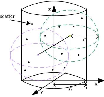
Fig. 1. Non-stationary property.
C. Non-stationary Property
Employing large antenna arrays, the non-stationary property have been observed through real world measurements [15], [16]. The non-stationary property refers to the fact that as an antenna array goes large, each antenna at different physical location has different perspective. GBSMs are often used to evaluate the performance of practical wireless communication systems in channel model standards, which accurately reflect the channel properties.
1) Cylinder Model and Spherical Visible Area Model
It’s assumed that all the scatters existing in the vicinity can be replaced by the equivalent scatters on the column surface of a cylinder. For a large-scale antenna array in both the transmitter and the receiver, not all the scatters can be seen by each antenna element, and different antenna element can see different scatters. The closer the two antennas are, the more common scatters they share. In order to characterize the non-stationary property and determine the scatters which can be seen by a particular antenna, a geometric method is proposed based on a cylinder model and a spherical model, as it shows in Fig. 1.
In the proposed geometric model, the visible range of each antenna is denoted by a virtual sphere, where the radius isr
and the center is the antenna itself. In this model, scatters on the surface of the cylinder can be seen by an antenna only if the distance between them is less than r. Therefore, each antenna element has a different set of visible scatters. In this paper the sphere radii of the antennas in the transmitter and the receiver are denoted asrtandrr, respectively.
2) Radius of the Spherical Visible Area
From the measurement results shown in [15], [16], we know that for a particular distance between two antenna elements, the correlation of their channel impulse responses can be seen as a constant value. The value reflects the grade of their sharing scatters. According to the distance and the correlation value, the radius of the sphere can be calculated.
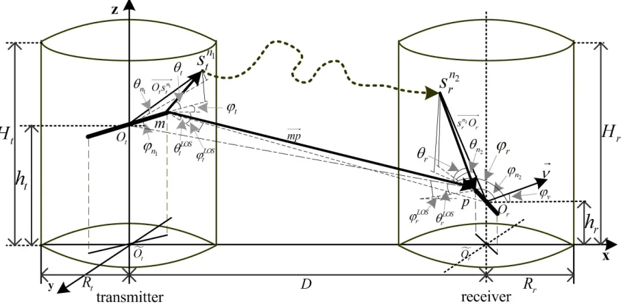
Fig. 2. A 3D GBSM channel model for massive MIMO channels.
(λis wavelength). The channel impulse correlation coefficient is assumed to be 0.9. Scatters are supposed uniformly distribut-ed on the side surface of the cylinder, whose radius isR. The radius of the visible sphere isr. To simplify the calculations, the three-dimensional graphics can be expanded into a two-dimensional image. An approximate value can be got
r > R×2.7856. (1)
III. 3D GBSM CHANNELMODELFORMASSIVEMIMO CHANNELS
A 3D GBSM channel model for 5G massive MIMO chan-nels is proposed in this section. To the best of our knowledge, it is the first geometrical model for describing the non-stationary property in massive MIMO channel models. As illustrated in Fig. 2, the 3D two-cylinder scattering model contains Mt transmitting antenna elements and Mr receiver
antenna elements. All antennas are omnidirectional and are numbered asm= 1,2. . . , Mt, p= 1,2. . . , Mr,respectively.
Scatters are randomly distributed in space without considering the length of the path traveled. Each scatter can be determined by two parameters: azimuth angle and elevation angle. Path length is compensated by a time delay. As can be seen from the propagation scenario in Fig. 2, there are two sorts of propagation path: line-of-sight (LOS) and double-bounced propagation. The double-bounced propagations are achieved by the equivalent scatters distributed on the cylindrical surfaces of both the transmitter and the receiver. Different from the physical scatters, an equivalent scatter may include several physical scatters whose delays and angle domains are irresolv-able. The first bounces occur when the waves propagate from the transmitting antenna elements to the equivalent scatters at the source side. Similarly, the waves propagate from the equivalent scatters at the destination side to the receiving
antenna elements are the last bounces. The propagations from the equivalent scatters at the source side to those at the destina-tion side are abstracted as virtual links. The disappearing and restructuring processes are not considered in the virtual link, because each received path at the destination comes from the source. The scatters on the two cylinders are randomly paired to simulate the uncertain real environment. Equivalent scatters are characterized by amplitude, delay, random phase and so on. With the time goes by, the values of all the parameters update. It is worth noting that in order to significantly reduce the complexity in the 3D theoretical GBSM, other bounced paths are neglected because they show similar channel statistics. Only the geometry of LOS components and the double-bounced two-cylinder model is illustrated in Fig. 2.
In order to simplify the analysis, a uniform linear antenna array with Mt = Mr = 2 is adopted as an example. The
antennas in proposed model can be extended to arbitrary numbers and the two antenna arrays can be constructed by any shapes. The two cylinders are located on a XoY plane in a 3D coordinating system, and the antenna arrays are parallel to the XoY plane. It is assumed that there areNtequivalent scatters
lie on the surface of cylinder at the source side, the radius of the cylinder is denoted by Rt and then1th (n1= 1, . . . , Nt)
equivalent scatter is denoted by sn1
t . Similarly, there are
Nr equivalent scatters lie on the surface of cylinder at the
destination side, where the radius of the cylinder is Rr and
n2th (n2 = 1, . . . , Nr ) equivalent scatter is denoted by snr2.
Note that the reasonable assumptionsD≫max(Rt, Rr), and
min(Rt, Rr) ≫ max(δt, δr) are applied in this theoretical
model, where D is the distance between the transmitter and the receiver on the XoY plane and δt, δr are the minimum
on the two cylinders is determined by the azimuth angle and the elevation angle. The azimuth and elevation angles of the scatters in the source side are donated by φn1 and θn1,
respectively, and those in the destination side are denoted by
φn2, andθn2.HtandHrare the heights of the cylinders in the
source and destination side, ht andhr are the heights of the
antenna array in the source and destination side. It’s obvious thatHt≫ht,Hr≫hr,Rt≫
√
Mtδt,Rr≫
√
Mrδr.fmax
is the maximum Doppler frequency. It is assumed that the number of the signal propagation paths is N and each path has a power Pn ( n = 1,2, . . . , N), and
∑N n=1
√
Pn = 1.
The initial phaseψ0is independent and identically distributed
(i.i.d.) random variable with uniform distribution over[0,2π), and the LOS Rician factor is K. The geometrical parameters are list in Table I.
The 3D massive MIMO channel model is described by an Mt×Mr matrix with complex fading envelopes, Ht =
[hmp(t)]Mt×Mr. The received complex fading envelope
be-tween themth and thepth antenna at the frequency offc is a
superposition of the LoS and the double-bounced components, which can be expressed as
hmp(t) =hLOSmp(t) + N
∑
n=1
hnmp(t), (2) where
hLOSmp(t) = √
K K+ 1exp
{ j
( ψ0+
2π λ|−→mp|
+ 2πfmaxt⟨−→ mp·⃗ν⟩
|−→mp| · |⃗ν| )}
, (3)
where−→·donates vector,⟨·⟩donates inner product,|·|donates module and
hnmp(t) = √
Pn
K+ 1exp {
j [
ψ0+ 2πfmaxt⟨
−−→
sn2
r p·⃗ν⟩
|−−→sn2
r p| · |⃗ν|
+2π λ (|
−−−→
msn1
t |+|
−−→
sn2
r p|+|sg n1
t s n2
r |)
]}
. (4)
IV. CHANNELMODELING ANDSIMULATIONPROCEDURE
A. Channel Modeling Process
The channel modeling process is described as Alg. 1. The procedure in line 7 is used to achieve the non-stationary prop-erty. The purpose of line 8 is to simulate signal propagation path. Finally, the channel matrix can be calculated in the final step.
B. Evaluation of Statistical Properties of the Massive MIMO Channel Mode
Based on our 3D two-cylinder GBSM channel model, it is possible to derive the corresponding statistical properties, including spatial cross-correlation function (CCF), temporal autocorrelation function (ACF), Doppler power frequency density (DSP) and condition number. With these statistical properties, the performance of the proposed channel model can be evaluated.
Algorithm 1 channel modeling process
1: Set the parameters for cellular scene, double-cylinder model and antenna model, respectively;
2: forNumber of simulation timesi∈[1, Ntimes] do
3: Substitute scatters into equivalent scatters on the surface of the cylinder at the initial time at both source and destination side, respectively;
4: Apply the parameters such as the angle distribution, delay spread in 3GPP 3D MIMO channel model for easy comparison and analysis;
5: Place these scatters on the surface of the two cylin-ders, the joint angular distribution consists of azimuth and elevation angles, which are modelled as wrapped Gaussian and Laplacian distribution respectively [1]; 6: forThe time course t∈[1, T] do
7: Compute every set of the scatters that can be seen by each antenna at both transmitter and receiv-er, respectively. The scatters can be expressed as
sn1
t , s n2
t ,(n1= 1, . . . , Nt, n2= 1, . . . , Nr);
8: Pair each path from transmitter to receiver with respect to the scatters on the two cylinders;
9: Apply the parameters such asφ, θ, ψ0 to each path;
10: Calculate the channel matrix for LOS hLOS
mp(t) and
NLOS hnmp(t) independently, and get the channel
matrixhmp(t)andHt instantly.
11: end for
12: end for
1) Spatial Cross-Correlation Function
Spatial correlation characteristics and time-related charac-teristics simultaneously exist in any fading channels. Spatial correlation is used to evaluate correlation between different antennas, and time-related correlation reflects the autocorrela-tion characteristics of a single receiving antenna at different time. The correlations in fading channels affect each other. In order to analyze the spatial correlation or the time-related correlation easily, when analyzing the spatial correlation, we do not take the time-related correlation into consideration. By settingτ = 0, the spatial-temporal correlation function reduces to the spatial cross-correlation (CCF) function
Rhmp,hm′p′(t) =
E[hmp(t)h∗m′p′(t)]
√
E[|hmp(t)|2]E[|hm′p′(t)|2]
=RhLOS
mp,hLOSm′p′
(t) +RhNLOS
mp ,hNLOSm′p′
(t), (5)
where(·)∗ denotes the complex conjugate operation andE[·]
represents the expectation value,
RhLOS
mp,hLOSm′p′(t) =
K K+ 1exp
{ j2π
λ (
|−→mp| − |−−→m′p′|)}
×exp {
2πfmaxt
(⟨−→mp·⃗ν⟩
|−→mp| · |⃗ν|−
⟨−−→m′p′·⃗ν⟩
|−−→m′p′| · |⃗ν| )}
TABLE I
DEFINITION OF THE PARAMETERS USED IN THE PROPOSED MODEL
Parameters Meaning
Ot, Or,Oet,Oer The center of the antenna array and their projection on XoY plane of transmitter and receiver, respectively.
Ht, Hr, Rt, Rr The heights and radii of cylinders at transmitter and receiver, respectively.
D The distance between transmitter and receiver on XoY plane.
ht, hr, δt, δr The heights of the antenna array and the inter-element distances at the transmitter and receiver, respectively.
Mt, Mr, m, p The numbers of the antennas at transmitter and receiver, respectively.
m= 1, . . . , Mt, p= 1, . . . , Mr
Nt, Nr The numbers of the scatters at transmitter and receiver, respectively.
sn1
t , s n2
t The specific scatter at transmitter and receiver, respectively.
n1= 1, . . . , Nt, n2= 1, . . . , Nr
φn1, θn1, φn2, θn2 The azimuth angle and elevation angle with respect toOt, Or at transmitter and receiver, respectively.
−−−−→
Otsnt1= [Rtcosφn1, Rtsinφn1, Rtcosθn1],
−−−−→ sn2
t Or= [Rrcosφn2+D, Rrsinφn2, Rrcosθn2].
⃗
ν, ν, φν The velocity vector for the receiver, the size and direction with respect toOr areνandφν,
⃗
ν= [νcosφν, νsinφν,0].
fmax The maximum Doppler frequency shift.
−−−→ msn1
t , φt, θt The direction vector from antennamto scattersnt1, including azimuth angle and elevation angle.
−−→ sn2
r p, φr, θr The direction vector from scattersnr2 to antennap, including azimuth angle and elevation angle.
−→
mp, φLOSt , θLOSt , φrLOS, θLOSr The LOS direction vector from antennamto antennap,
including azimuth angles and elevation angles at the transmitter and receiver, respectively.
K Rice factor for LOS.
ψ0 The initial phase of the path.
Pn(n= 1,2, . . . , N) The power of each path.
rt, rr Radii for the non-stationary property at the transmitter and receiver, respectively.
and
RhNLOS
mp ,hNLOSm′p′ (t) =
√ P K × N ∑ n=1 M ∑ m=1 exp {
j2π λ∆s
+2πfmaxt (⟨−−→sn2
r p·⃗ν⟩
|−−→sn2
r p| · |⃗ν|
− ⟨ −−−→
sm2
r p′·⃗ν⟩
|−−−→sm2
r p′| · |⃗ν|
)}
. (7)
2) Temporal Autocorrelation Function
Autocorrelation function expresses the dependencies of each other in the same process between different moments. Here, by setting m′ =m,p′=p, we can get temporal autocorrelation function
Rhmp(τ) =
E[hmp(t)h∗mp(t−τ)]
√
E[|hmp(t)|2]E[|h∗mp(t−τ)|2]
=RhLOS
mp(τ) +RhNLOSmp (τ), (8)
where LOS component is
RhLOS
mp(τ) =
K K+ 1exp
{
2πfmaxτ ⟨−→ mp·⃗ν⟩
|−→mp| · |⃗ν| }
, (9)
and NLOS component is
RhNLOS
mp (τ) =
N ∑ n=1 M ∑ m=1 √ P Kexp {
−2πfmaxτ
⟨−−−→sm2
r p·⃗ν⟩
|−−−→sm2
r p| · |⃗ν|
+j2π
λ ∆s+ 2πfmaxt (
⟨−−→sn2
r p·⃗ν⟩
|−−→sn2
r p| · |⃗ν|
− ⟨ −−−→
sm2
r p·⃗ν⟩
|−−−→sm2
r p| · |⃗ν|
)} . (10)
3) Doppler Power Frequency Density
Channel characteristics change as the signal propagating, resulting in selective fading. A time-selective fading channel is caused by the relative motion between the mobile station and the base station, or caused by the moving of objects in
the path. Different antennas on the same array will experience different Doppler shifts because of the spherical propagation of the signal. Therefore, Doppler frequencies may vary on the antenna array. Applying the Fourier transform to the spatial-temporal correlation function, we can obtain the corresponding Doppler PSD
Shmp,hm′p′(fD) =F{Rhmp,hm′p′(τ)} =
∫ +∞
−∞
Rhmp,hm′p′(τ)e
−j2πfDτdτ, (11)
wherefDis the Doppler frequency,F donates Fourier
trans-form, and
Shmp,hm′p′(fD) =F{RhLOSmp,hLOSm′p′
(τ)}+F{RhNLOS
mp ,hNLOSm′p′ (τ)}
=F{RhLOS
mp,hLOSm′p′(τ)}+F{R
T
mm′(τ)} ⊙F{RRpp′(τ)}, (12)
where⊙donates the convolution.
4) Condition Number
Condition number is a key measurement of the correlation of the channel matrix [3]. If it has higher correlation, there will be larger condition number. The condition number is related to the eigenvalue of the channel matrix.
c(dB) = 20 log10λmax(H) λmin(H)
, (13)
where λmax represents the maximum eigenvalue and λmin
represents the minimum eigenvalue.
V. RESULTS ANDDISCUSSIONS
Fig. 3. The absolute value of the ACF.
frequencies of 2GHz and 28GHz are included in the simulation separately. The distance between the base station and the mobile station is D= 200m. The minimum spacing between two antennas is δ =λ/2. The radii of the cylinders on both sides are R = 25m, and the radii of the spheres used for the non-stationary properties are r = 70m. The heights of antenna arrays at the base and mobile station are hT = 32m
andhR= 1.5m, respectively. The values and distributions of
parameters used in this paper come from the 3GPP standard [1].
The absolute values of the temporal ACF are analyzed in Fig. 3. The figure shows that the temporal ACF decreases lower as the time pass. From the figure we observe that the proposed model has similar change trend with the 3GPP model both in 2GHz and 28GHz. It is because scatters in proposed model and 3GPP model update every moment along the time axis, part of the scatters remained while part of the scatters be replaced by new scatters, the difference between the two models is the number of scatters can be seen, it costs a slight difference.
By setting time to zero, the impacts of the absolute value spatial correlation function are depicted in Fig. 4. Decreasing trends can be observed while the normalized antenna spacing increasing at the receiver side. Spatial correlation with insta-bility caused by the massive antenna elements, the larger the distance between two antennas, the lower the spatial correla-tion they have. There are not big difference between 2GHz and 28GHz because they have the same antenna positions.
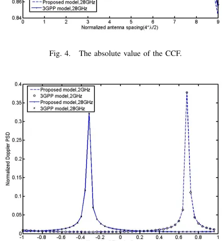
As the Doppler PSD is derived from the Fourier transform of corresponding temporal ACF, Fig. 5 shows the Doppler PSDs of the proposed 3D model in both 2GHz and 28GHz. Because of the non-stationary massive MIMO channel model on the time axis, the PDFs of Doppler frequency at a time instant vary instead of symmetrical with respect to 0. The physical reason is that the relative movements of the receiving side receives the signal from different directions, and the larger components of the received signal power are from LOS components and the
Fig. 4. The absolute value of the CCF.
Fig. 5. The normalized Doppler PSD.
static components in the real scattering environment. Doppler PSDs depend on the wavelength and time domain, so they are different in 2GHz and 28GHz.
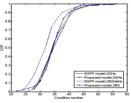
A comparison of condition numbers between the 2GHz and 28GHz models is shown in Fig. 6. Stronger correlations are observed in 3GPP model than the proposed model due to the fact that clusters have higher probabilities to be correlated in 3GPP model. And stronger correlations are observed in the 28GHz model than the 2GHz model, antenna spacing with 2GHz is larger than 28GHz, so it has higher probabilities to see new scatters than 28GHz. But the difference is small because scatters’ locations are randomly distributed in space.
Fig. 6. Conditional number.
For example, the heights of the cylinders can be got from the elevation range of the signal in vertical plane. Thirdly, the proposed model has good applicability, and it is easy to fit kinds of experimental data. Finally, the proposed model has good compatibility with the general channel model standards.
VI. CONCLUSIONS
For the large antenna array employed in 5G, there will be three important properties in the massive MIMO model: 3D MIMO, spherical wave effect, and especially the non-stationary property. Considering these three properties, a 3D geometry-based stochastic model for 5G massive MIMO chan-nels is proposed in this paper. Using the equivalent scatters which lie on the side surface of the cylinder, it’s convenient to simulate the practical scatters. Most importantly, a geometry method is used to achieve non-stationary property. The visible range of each antenna is denoted by a sphere with itself in the center. In order to evaluate the validity of the proposed model, the statistical properties have been derived and inves-tigated. Compared with the 3GPP 3D MIMO channel model, the proposed model have close agreements in the statistical properties with 3GPP channel model. The proposed 3D GBSM massive MIMO channel model is effective to evaluate the 5G communication systems. The proposed model is easy to implement, and provides another effective solution for the modeling of 5G massive MIMO channels.
ACKNOWLEDGMENT
This work is supported in part by the National Natu-ral Science Foundations of CHINA (Grant No. 61271279, and 61201157), the National 863 plans project (Grant No. 2014AA01A707, and 2015AA011307), the National Science and Technology Major Project (Grant No. 2015ZX03002006), and the Fundamental Research Funds for the Central Univer-sities (Grant No. 3102015ZY038, 3102015ZY039).
REFERENCES
[1] “Technical specification group radio access networkstudy on 3D channel model for LTE (Rel 12),” 3GPP TR-36.873, Tech. Rep., Sep. 2014. [2] S. Alamouti, “A simple transmit diversity technique for wireless
commu-nications,”IEEE J. Sel. Areas Commun., vol. 16, no. 8, pp. 1451–1458, Oct. 1998.
[3] E. Larsson, O. Edfors, F. Tufvesson, and T. Marzetta, “Massive MIMO for next generation wireless systems,” IEEE Commun. Mag., vol. 52, no. 2, pp. 186–195, Feb. 2014.
[4] C.-X. Wang, F. Haider, X. Gao, X.-H. You, Y. Yang, D. Yuan, H. Ag-goune, H. Haas, S. Fletcher, and E. Hepsaydir, “Cellular architecture and key technologies for 5G wireless communication networks,”IEEE Commun. Mag., vol. 52, no. 2, pp. 122–130, Feb. 2014.
[5] K. Zheng, S. Ou, and X. Yin, “Massive MIMO channel models: A survey,”International Journal of Antennas and Propagation, 2014. [6] J. Hoydis, S. ten Brink, and M. Debbah, “Massive MIMO in the UL/DL
of cellular networks: How many antennas do we need?”IEEE J. Sel. Areas Commun., vol. 31, no. 2, pp. 160–171, Feb. 2013.
[7] L. Lu, G. Li, A. Swindlehurst, A. Ashikhmin, and R. Zhang, “An overview of massive MIMO: Benefits and challenges,”IEEE J. Sel. Top. Sign. Proces., vol. 8, no. 5, pp. 742–758, Oct. 2014.
[8] S. Wu, C.-X. Wang, E.-H. Aggoune, M. Alwakeel, and Y. He, “A non-stationary 3-D wideband twin-cluster model for 5G massive MIMO channels,”IEEE J. Sel. Areas Commun., vol. 32, no. 6, pp. 1207–1218, June 2014.
[9] A. Kammoun, H. Khanfir, Z. Altman, M. Debbah, and M. Kamoun, “Survey on 3D channel modeling: From theory to standardization,”
ArXiv Preprint, 2013.
[10] K. Yu and B. Ottersten, “Models for MIMO propagation channels: a review,”Wireless Communications and Mobile Computing, vol. 2, no. 7, pp. 653–666, 2002.
[11] “Spatial channel model for multiple input multipleoutput (MIMO) simulations,” G. T. S. ,25.996, V11.0.0, Tech. Rep., 2012.
[12] WINNER II interim channel models, IST-WINNER Std., 2006. [13] F. Wang, X. Cheng, L. Yang, B. Yu, and B. Jiao, “On the achievable
capacity of dual-polarized antenna systems in 3D indoor scenarios,” pp. 605–610, Aug. 2013.
[14] J. Parsons and A. Turkmani, “Characterisation of mobile radio signals: model description,”IEE Proceedings I: Communications, Speech and Vision, vol. 138, no. 6, pp. 549–556, Dec. 1991.
[15] S. Payami and F. Tufvesson, “Channel measurements and analysis for very large array systems at 2.6 GHz,” pp. 433–437, Mar. 2012. [16] X. Gao, F. Tufvesson, O. Edfors, and F. Rusek, “Measured propagation