A process planning system for cold extrusion
SANTOSH KUMAR*
Department of Mechanical Engineering, Institute of Technology, B.H.U. Varanasi (INDIA) 221005 RAHUL KUMAR
Department of Mechanical Engineering, Institute of Technology, B.H.U. Varanasi (INDIA) 221005 J.P.DWIVEDI
Department of Mechanical Engineering, Institute of Technology, B.H.U. Varanasi (INDIA) 221005 Abstract
A Process Planning system ProEx-Cold is developed for extrusion shapes to eliminate the tedious and expensive procedure of trial and correction of a proper die and the process. The system has three modules as: feature recognition, upper bound analysis and 3D graphics generation & display using OpenGL application engine. The input parameters to the proposed CAPP system includes: die type, billet TYPE & material, geometrical details of the product, ram speed, reduction, friction condition and billet condition etc. to influence parameters like production rate, extrusion ram pressure etc. C-programming, OpenGL graphics and Visual C++ editor has been used to implement ProEx-Cold. Keywords: Extrusion, process planning, Upper bound technique, OpenGL graphics
.
1. Introduction
Planning has been traditionally carried out manually based on experience and in isolation from the actual manufacturing. Presently it is being performed with the help of computers leading to computer aided process planning (CAPP). There are numerous factors that affect process planning of cold extrusion such as extrudate shape & size, tolerance, surface finish, component type, material and quantity to manufacture, etc. The process planning contributes towards selection of dies, operative parameters, their manufacturing sequence and determination of the design and manufacturing parameters.
The process planning procedure in past has been dependent on the experience and judgment of the planner. It is the responsibility of manufacturing engineers to determine the optimal process parameters for each part design. However, individual engineers have their own opinions about what constitutes the best practice & routings. Accordingly, there have been differences among the operation sequence developed by different planners. Because of these problems encountered with manual process planning, an attempt has been made to capture the logic, judgment and best experience required for this important function and to incorporate them into suitable computer programs [1, 2, 3, 4, and 5]. Automation of process planning [6, 7, 8, 9, and 10] with computers has led to several advantages, such as reduced lead time, visualization, better efficiency, improved quality, and reduced cost associated with production and planning of Extrusion process.
The alternative approaches available to computer-aided process planning have been Variant-type CAPP systems, retrieval, semi-generative CAPP systems and generative CAPP systems. Retrieval-type CAPP systems use part classification and coding system in group technology as a foundation. In this approach, the parts being produced are grouped into part families and are distinguished according to their manufacturing characteristics. For each part family, a standard process plan is established. The standard process plan is stored in computer files and then retrieved for new work parts, which belong to the family. CAM-I CAPP [11] is one of the well-known examples of such CAPP systems. Semi-generative CAPP systems are advanced variant systems, incorporating quasi-generative features. After the part family has been identified, as in the basic variant system, these systems offer the user several options like: (i) make suitable changes to the standard process plan for each part family, (ii) begin with an incomplete process plan and complete it for a specific part, and (iii) start from the beginning and completely create a new process plan by using various standard process descriptions stored in the computer.
without human assistance. The computer would employ a set of algorithms to progress through the various technical and logical and graphical decisions towards a final plan. Input to the systems would include a comprehensive description of the work part and process details. Wyask [14] and Kotler [15] are some of the systems of this kind. The review work on CAPP application by Santosh et al. [16] shows that there are several areas of CAPP applications as: machining, Sheet metals, Unconventional manufacturing processes, Grinding, forging etc.
The available literature on CAPP application in metal forming shows that no full effort has been made to develop a user friendly CAPP system for cold extrusion die design with graphical visualization of the extrusion process. The aim of the present work is to develop a menu-driven interactive CAPP system ProEx-Cold through single-hole die for cold extrusion process (Gunasekhera [17], Kumar et .al. [16, 18] and Kumar [19]). The present CAPP system is capable of predicting optimal process conditions for cold extrusion of re-entry and non re-entry shapes. A suitable process plan sheet is the main output. The system also generates 3D drawings and views of complete extrusion die set to help the designer in choosing the best design.
2. Design and development of the CAPP system
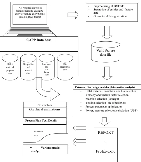
The aim of the proposed CAPP system ProEx-cold is to generate most economical process plan for solid extrudable components of simple or complex nature using single stage cold extrusion through a single-hole die. Fig. 1 shows the proposed CAPP system schematically, comprising of the following three major modules as (a) Feature recognition (b) upper bound analysis and (c) 3D graphics generation and display.
2.1. Feature Recognition,
The feature recognition deals with 2D based data pre-processing and data generation process using geometry recognition methodology based on product feature, billet feature and pocket feature as proposed by Kumar [1]. The data processing require geometrical data of the component (wire frame model) derived from a neutral AutoCAD file format such as DXF. The geometrical data from the DXF file is separated and collected in some file (data.p/data1.p/data2.p….). This file is further processed to generate various data files. Each vertex of the previously generated geometrical data file (data.p/data1.p/data2.p…) is zoomed and divided to acquire the required extruded profile dimensions. The final data is collected in “arbitrary.p” file. This data is further processed to have profile geometrical data (EPGD). The co-ordinates of the each vertex are calculated with respect to C.G. of EPGD data as in equation (1).
x
x
x
i
i
andy
i
y
i
y
(1)
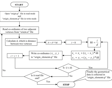
Finally the geometrical data is collected in “origin.p” file and is referred as extruded profile geometrical data with respect to C.G. (EPGDwrtCG). Dividing EPGDwrtCG into a number of small elements helps in creating accurate drawing of required profile die. Also as the upper bound analysis is to be used for extrusion process, finer the elements better is the results. The process of element generation is shown in flow chart Fig. 2. The non re-entry data so obtained is written to “origin_elements.p” and referred as EPGDwrtCGe.
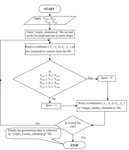
For generation of data for re-entry shape the above process of non re-entry shape data generation is adopted with some strategy. The geometry of the re-entry component shape is broken into minimum number of sub components such that each of them represents a non re-entry shape (Fig. 3). Each of the sub-components so divided is again drawn using AutoCAD and saved as separate DXF files. Extra entities required for the proposed non re-entry shapes are recorded carefully. The extra entities need not require frictional power calculation. Care is taken so that the frictional power is calculated only once only along the entities of the re-entry shape. The procedure for generating elements corresponding to non re-entry shape is shown with a flowchart Fig. 4.
---
---
Fig. 1: Schematic diagram of proposed CAPP system ProEx-Cold
- Preprocessing of DXF file - Separation of entities and feature
data
- Geometrical data generation
Valid feature
data file
All required drawingscorresponding to given Re-entry or Non re-Re-entry Shape
saved in DXF format
Extrusion dies design modules (deformation analysis)
-
Billet material, condition, and Die selection-
Velocity and friction factor selection-
Machine selection (tonnage)-
Tooling selection (die accessories)-
Process parameter optimization-
Power, pressure selection/calculation (UBT)CAPP Data base
Billet material property data
Die profile and material
data
Lubricant and cost factor data
Die accessories
data
REPORT
–
ProEx-Cold
Graphical
animations
Various graphs Process Plan Text Details
Yes No
No
Yes
Fig. 2: Flow chart for generation elements corresponding to EPGDwrtCG. (1/M is the distance between two adjacent vertexes of ‘origin_elements.p’ file
All elements of the proposed non re-entry shape is inside the rectangle, and it is termed as extra elements to form extra entities. The final geometrical data is written to the “origin_reentry_elements.p” file and referred as (EPGDwrtCG)R
,
where ‘R’ stands for re-entry shape. The data generated from the DXF file require further processing for higher-level recognition (whether given shape is re-entry or non re-entry). The (EPGDwrtCG)e is used for higher level recognition
using a gradient test.
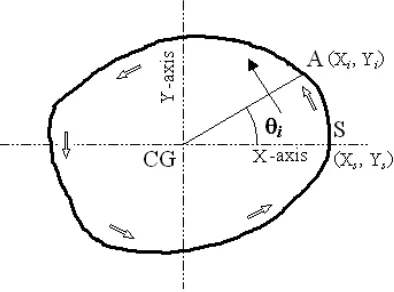
Fig. 5 shows a solid extrudable shape. The vertex (Xs, Ys) is first vertex of EPGDwrtCG. The starting vertex for the
gradient test is (Xs, Ys) and the gradient of this vertex is taken as zero. This is done by selecting the axes in such a way
that x-axis passes through CG and starting point of the shape (Xs, Ys) and y-axis passes through the CG and is
perpendicular to x- axis. To select axes in such a way, it requires rotation of the axes at some angle with respect to previous axes. If (xi, yi), where i= 1 to 3, corresponds to the co-ordinates of some vertex of the feature shape with
respect to previous axes then co-ordinates of that vertex with respect to new transformed axes are calculated as eqn. (2).
sin
cos
sin
cos
i i i i i ix
y
Y
y
x
X
(2)Where is the gradient of the vertex (Xs, Ys). The gradient of any point A (Xi, Yi) along the geometry of the
shape with respect to X-axis is obtained as eqn. (3). START
Open “origin.p” file in read mode and
“origin_elements.p” file in write mode
Read co-ordinates of two adjacent vertexes from “origin.p” file
Is it read file end? Calculate d, which is distance
between two vertexes
STOP
Finally the geometrical data is collected in “origin_elements.p” file d = d * M
d
i
kk
kk
y
y
y
y
kk
x
x
x
x
s e s s s e s s*
)
(
*
)
(
Write co-ordinates (
x
s,y
s) to “origin_elements.p” fileIs (i≤ d) i= 0
Proposed re-entry shape Proposed segments of the re-entry shape Proposed non re-entry shapes
Yes
No
No
Yes
Fig. 4: Flow chart for generating elements corresponding to non re-entry shape of a given re-entry shape Open “origin_elements.p” file in read
mode for proposed non re-entry shape
Is it read file end? Finally the geometrical data is collected
in “origin_reentry_elements.p” file.
Write co-ordinates (
x
s,y
s),(x
e,y
e) to “origin_reentry_elements.p” file Input: Xmax, XminYmax, Ymin
Is Xmin Xs Xmax
Ymin Ys Ymax
Xmin Xe Xmax
Ymin Ye Ymax
fpow = 0
fpow = 1
Read co-ordinates (
x
s,y
s),(x
e,y
e) of two consecutive vertices from the file
i i i
X
Y
1tan
(3)Thus by moving in anti-clockwise direction from the start vertex (Xs, Ys), the gradients of other vertices may be
found. If the gradients are in increasing order, the component shape layout is recognized as a non re-entry shape otherwise it is re-entry.
Inputs to the system
The module is used to select DXF file or files (in case of re-entry case), number of occurrence of the geometry in the final extruded shape (re-entry case), type of extrusion die, reduction required, velocity of ram, nature of component, billet condition, billet material, type of production etc. Fig. 1 shows structure of the proposed system ProEx-Cold. For further details on the inputs, one may refer Kumar et al. [18].
Fig. 5: Higher level recognition of a shape.
Outputs of the System
Fig. 6: Layout of process plan chart developed by proposed CAPP system.
2.2. Upper bound formulation
(Constitutive Equations)
Neglecting the elastic deformation, the strain rate tensor is given by
i j j i ijx
v
x
v
2
1
(4)Where viand vj represent the velocity components along xiand xjare the variables in the Cartesian coordinate system.
The constitutive law for rigid plastic/ viscoplastic material relating the deviatoric stress tensor
'ij and the strain rate tensor
ij is expressed asij ij
'2
(5)where µ is the Mises coefficient. For a material yielding according to Von-Mises criterion, the Levy-Mises coefficient is given by
3
(6)where the generalized yield stress
and the generalized strain rate
are defined as ' '2
3
ij ij
(7)and
ij
ij3
2
(8)
The generalized strain
is therefore, defined as
=
0 tdt
(9)where the integration is to be carried along the particle path. In general
depends on
,
and temperature T.)
,
,
(
T
F
(10)In case of cold extrusion, the effect of temperature is neglected on generalized stress
.The upper bound theorem states that among all possible kinematically admissible velocity fields, the one that minimizes the total power
T is the actual velocity field.i S t S ij ij
T
d
v
idS
i * * *
(11)In the above equation is the plastic deformation zone, is the shear stress on velocity discontinuity surfaces Si . The Upper bound solution is based on certain assumptions [20]. Since deformation is under certain assumptions and
streamlines are the basic flow path during the deformation process, it is necessary to build the proposed kinematically admissible velocity using streamlines concept. The geometry of die and the velocity field in terms of streamlines in the steady flow process of extrusion is shown in Fig. 7.
One power element O′E′1E1E2E′2O′ is chosen to demonstrate the analytical construction of the velocity and strain
rate fields. In Fig.7, billet with initial radius is given by (Ro) at entry, is extruded through a shaped die (continuous)
the exit. An arbitrary point E′1 on the die surface at the entrance of the die can be combined with the corresponding
point E1 on the die surface at the exit. The surface defined by the points O, E′1, E1, and E2 E′2O' becomes a
three-dimensional stream surface.
Assumptions (i) and (ix) state that the reduction ratio is kept constant while the subdivision of the domain into small elements. Analyzing one such power element O'E′
1E1E2 E′2O'(Fig. 7).
side
billet
on
area
section
cross
ABCD
rectangle
of
Area
side
product
on
area
section
cross
D'
C'
B'
'
rectengalA
of
Area
(12)If the coordinates of points E′1andE′2 and E2 are (x1, y1), (x2, y2), (x3, y3) and (x4, y4) respectively and Aa is the
cross-sectional area of the extruded product shape.
Then, O´ E′1= a1 =
x
12
y
12
O´E′2 = a2 =
x
22
y
22
. O´E1 = a3 =
x
32
y
32
O´E2 = a4 =
x
42
y
42
4 3 1 2 1
cos
a
a
b
a
a
b
Whereb
x
1x
2
y
1y
2
andb
1
x
3x
4
y
3y
4
from Eq. (11),
2 2
2 2 4 3 2 1
2
2
sin
2
1
sin
2
1
i o i oa
R
R
R
R
A
a
a
a
a
and
.
=
sin
4 3 2 1 aa
a
a
a
A
. (13)The streamlines on the stream surface is represented by a fourth order polynomial to satisfy the smooth entry and exit of the material flow. Any coordinate along the streamline EE´ is formulated in a Cartesian coordinate system as follows: z z c z c z c z c z c z f y b b z b z b z f x 5 4 2 3 3 2 4 1 = ) ( 2 5 b z 4 + 2 z 3 3 2 4 1 = ) ( 1 (14)
Where
b
iandc
i (for i = 1, 2, 3, 4 and 5) are constants, determined by the boundary conditions. Since the streamline does not produce any abrupt change in flow direction along the extrusion axis at entry and exit, the boundary conditions can be written as
cos ; = 0 at product side ( ) 0 = ; sin 2 2 L z z y R a n R y z x R a n R x o i o i
(16)where
R
ois the billet radius, and are the angles between the plane of symmetry and the stream surface at entry and exit of the die respectively and L is the die length, Ri is the mandrel radius at entry.Substituting these boundary conditions from Eq. (15) and (16) into Eq. (14) gives
z z z f R a n c n y z f R a n n x o e e o e e ) ( cos cos os ) ( sin sin sin 2 2
(17)L
z
z
f
z
z
f
at
1
)
(
and
0
at
0
)
(
where
(18)and
n
e=R
i
n
In the present analysis, function f is represented by the following fourth order curve.
4 3 3 4 ) ( L z L z z f
f (19)
Equation (19) describes the coordinate inside the plastically deforming region but the relationship between the Cartesian and n,, z coordinate systems also. Although the present analysis employs a fourth order curve represented by equation (14) for the description of die profile and the assumed streamlines of particles, it is to be noted that function f in equation (18) can be any general function of z provided the function satisfies the given boundary conditions.
The Jacobian of equation (17) can be found as
z
z
z
y
z
x
z
y
x
n
z
n
y
n
x
J
(20)Where
sin
A
; 2A
;
R
con
a
B
o
4 3 2 1a
a
a
a
A
con
;C
cos
andR
C
a
D
o
2cos
(22)Hence
1
'
'
0
'
'
'
'
0
Df
n
Bf
n
f
D
n
C
n
f
B
n
A
n
Df
C
Bf
A
J
e e e e ee (23)
Determinant of the Jacobian is therefore written as
det J = ne. g (, z), (24)
Where g(,z)
ABf
C'D'f
A'B'f
CDf
(25)Strain rate components
ijare represented by equation (4).
Where vi and vj represent the velocity components along xi and xj axes in Cartesian coordinate system
respectively. The partial derivatives of the above equations are obtained with the help of coordinate transformation as:
3 1 k j k k i j ix
u
u
v
x
v
(26)Assuming that the plastic zone is bounded by entry and exit shear surfaces, the velocity field components can be obtained. Because of volume continuity, the velocity component along z-direction in the Cartesian coordinate system (vz) should be vo at the entrance, and vpat the exit of die. voand vpare the speeds of the billet and the outgoing product
respectively. vpcan be described in terms of voas
oi o p
v
a
a
a
a
R
R
v
sin
2
1
2
4 3 2 1 2 2
(27)These requirements are satisfied using equation (21) and (22). Therefore, other velocity components for incompressible material are determined as
o z o e y o e x
v
z
g
v
v
z
g
Df
n
v
v
z
g
Bf
n
v
)
,
(
1
)
,
(
'
)
,
(
'
(28)i.e.
(
.xx +
.yy +
.zz) = 0.
hence, the proposed velocity field model fulfils the stringent requirement for the construction of a kinematically admissible condition.
The generalized yield stress
at any point in the deformation zone is calculated using the value of generalized strain
at that point using equation (9). Since the material enters the die as a rigid body, the generalized strain
is taken as zero on the entrance boundary of the die. Integration of
is performed using ten point Gauss Quadrature rule to find the cumulative generalized strain along each streamline. The total power consumed inside the die (Fig. 7) is the sum of total power consumed due to various power elements. Total power (T) consumed within the element is given asT = i + e + o + f + int (29)
where i is the power loss due to internal plastic deformation, eando are powers due to velocity discontinuities at
entry and outlet of the die, and f is the friction power loss along the interface between the material and the die. If o is
the yield stress of the material (neglecting strain hardening effects), the power components of eqn. (15) can be obtained as
i
ij ij
Ro
L
dn d dz
2
3
0
0
0
05
1
2
_
.
det J
(30)
e o V x V y
z Ro
n d n d
3 2 2 0 1 2 0
0 (31)
o o Vx Vy z L
R
nC a Ro dn d
3
2 2 12
0 0
12 2
o (32)
d
dz
z
z
x
L
o
R
n
z
V
y
V
x
V
m
f
(
,
)
)
,
(
cos
1
0 0
2
1
2
2
2
3
(33)
o
Δ
V
i
A
i
3
int
(34)Here,
i
A is area of the ith interface formed by the coordinate points (0,0,L), (x, y, L), ( sin
o
R ,Rocos
,0) and (0,0,0). The velocity discontinuity (i
ΔV ) developed at the ith interface due to relative velocity of ith and (i-1)th elements is
evaluated as
i
ΔV = (
1 fi V fi
V ), where
fi V and
1
fi
V are average tangential velocity of ith and (i-1)th elements. For
ith element,
fi
V is evaluated as [ ( ) ]/2
i f V o V fi
V .
Therefore, for n power elements, the total interface power (
inttot) is
n i itot o ΔViA
1 int
3
.The overall power (o) is the sum of powers (T1, T2, T2 etc.) consumed in various power elements of the shape.
From the overall power (o) consumed during extrusion, the upper limit of the average ram pressure (Pave ) and the
relative forming stress (Rs) for the extrusion are found as
Pave o / ( ); R o Vo2 R s Pave / o (35) The optimal die length for a non re-entry shape is selected corresponding to minimum extrusion power consumption. Die length for a re-entry shape has been found to be optimum when the sum of total power consumption for all proposed non re-entry shapes of the re-entry shape is minimum.
The procedure mentioned is used to find deformation power and die design is done on the basis of optimum conditions. The above procedure is used for re-entry as well as non re-entry shaped profiles.
Process Plan Output
The output of the proposed CAPP system is shown with the help of a process plan chart (Fig.6). 2.3. Generation of 3D Graphics for Extrusion
The first phase of production process starts from the design part and then to the production department. The 3D drawing of the die, billet and final product is created using OpenGL [21] to help die designer in understanding the extrusion process. The process plan includes graphical viewing and simulation of the process to minimizing the time taken to gather required information from it. The generations of graphs between various process parameters also help in revealing the hidden aspects of die design through parametric study.
The generation of 3D drawing of dies with required profile and final cross-section is done using openGL graphics & visual C++ editor. A flat die is generated with the help of well-defined OpenGL functions like disk and cylinder. The
tessellated function helps in creating the required imported cross-section from AutoCAD. Die Profile Generation for Non re-entry and Re-entry Component Shapes
For generating a non re-entry shape the points on the periphery of the die inlet are calculated corresponding to the gradient of the points on the extrudate profile. The points are then joined with each other corresponding to points on the extrudate profile in form of quadrilaterals to form the die profile. For a non re-entry shape, every point of the extrudate profile has unique co-ordinates so one calculate the points on the periphery of the die inlet corresponding the gradient of the points on the extrudate profile, and then the corresponding points are joined on the extrudate profile to form the die. But since in case of re-entry component shapes, two or more points can have same gradient so it becomes quite difficult or sometimes impossible to generate the die with required profile. Therefore, the periphery of the die inlet is divided into some number of points, with gradient of the points increasing in linear manner. The process required for die profile generation is illustrated with the help of a flowchart Fig. 8.
Billet Generation
The procedure for generating the billet profile corresponding to selected die is same as the case for generating a extrusion die without need of generating cylindrical and disk shapes, as used to form the die case.
Billet animation
The animation technique provides a better way to understand the phenomenon involving in the process of design. The procedure concept used in the present CAPP system to animate the billet is explained as below. It is assumed that billet enters from the left hand side and let, t1, t2 be the time variables.
1 1
V
A
t
,2
2
V
L
t
V1= Billet speed before entering the die or ram speed
V2 = Billet speed inside the die (though it changes at every position inside the die, here it is taken as a value
somewhat more than V1 for viewing purpose).
Now let V3 be the speed of the extrudate and B be the billet length, Time be a variable representing current state of
time. Initial value is taken as zero. The animation of the billet is divided into the following three stages: Stage I – Animation of the billet (that has to enter on the left of the die inlet).
Stage II – Animation of the billet (that is inside of the die). Stage III – Animation of the extrudate coming out of the die. Stage I
If Time < t1
D = A – V1*Time
If Time t1
D = B – V1*(Time – t1)
Stage II
If t1 Time t1 + t2
E = E + V2*(Time – t1)
Where E is a variable having zero initial value.
If Time > t1 + t2
E = die length. Stage III
If Time > t1 + t2
F = F + V3*(Time – t1 – t2)
Graphs Generation
The present CAPP system is capable of generating graphs between various extrusion parameters. The program is to be executed a number of times and each time different parameter is selected for increasing input parameters. The result is visually shown in graph form.
Process Plan Generation
The present CAPP system has been used to generate the output in form of a process plan for the particular extrusion case. The process plan layout looks like as shown in Fig. 7.
Render the round billet with left end of the billet at a
distance of (
B+ D
) and right end of the billet at a
distance of
B
from the die inlet.
Render the round billet with left end of the billet at a
distance of
D
from the die inlet and right end of the
billet at the die inlet.
Render the required profile billet with left end at die
inlet with radius = billet radius and right end at a
distance of (-
E
) from die inlet.
X Y
Z
X
1
R o
1
o
a2
s1
E
o
o
E
E E
E
E
E
1 2 3
4 5
7 8
s
x-
z
p l
a n
e
1
E n la rg ed
E E
E E
E
E
E8
7 5 4 3
2
E
, ,
, ,
,
, ,
Y
a
Fig. 7: Relationship between die surface and projected surface [Santosh et. al. 2003].
2.4. System Implementation
The present CAPP system ProEx-Cold has been designed and implemented using the procedure as proposed in the previous sections. The ProEx-Cold code has been developed with the help of OpenGL graphics API along with C++
language. While implementing the CAPP system, following thee assumptions are made. (i) DXF file consists of line or point entities only (ii) DXF file is generated in anticlockwise direction and geometrical data in it should start from a vertex, which has +ve x co-ordinate and y co-ordinate as zero and (iii) the database obtained generated from various reliable sources.
In the present CAPP system, inputs may be changed, either by clicking the mouse and moving it around or by keyboard click or by selecting the required input from the menu itself. Most of the things in the present CAPP system are self-explanatory. But user requires a sound knowledge of extrusion process. Operating with the keyboard provides sometimes a simple and better way to use ProEx-Cold. Following are some of the keyboard commands implemented.
g – Starts user bound analysis for selected parameters.
p – Displays process plan for selected parameters.
d- Displays die.
b – Displays billet.
m – Shows moving billet.
v – Decreases extrusion ram velocity by a step of 0.001.
V - Increases extrusion ram velocity by a step of 0.001.
f - Decreases friction factor by a step of 0.01.
F - Increases friction factor by a step of 0.01.
z - Decreases zoom factor by a step of 0.001.
Z - Increases zoom factor by a step of 0.001.
r - Decreases percentage reduction by a step of 0.1.
R - Increases percentage reduction by a step of 0.1.
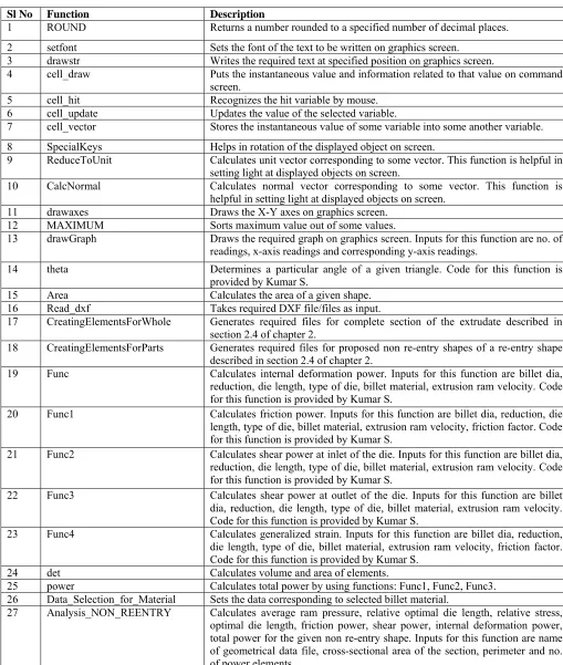
Table 1: Functions used to implement the CAPP system ProEx-Cold.
Sl No Function Description
1 ROUND Returns a number rounded to a specified number of decimal places. 2 setfont Sets the font of the text to be written on graphics screen.
3 drawstr Writes the required text at specified position on graphics screen.
4 cell_draw Puts the instantaneous value and information related to that value on command screen.
5 cell_hit Recognizes the hit variable by mouse.
6 cell_update Updates the value of the selected variable.
7 cell_vector Stores the instantaneous value of some variable into some another variable. 8 SpecialKeys Helps in rotation of the displayed object on screen.
9 ReduceToUnit Calculates unit vector corresponding to some vector. This function is helpful in setting light at displayed objects on screen.
10 CalcNormal Calculates normal vector corresponding to some vector. This function is helpful in setting light at displayed objects on screen.
11 drawaxes Draws the X-Y axes on graphics screen.
12 MAXIMUM Sorts maximum value out of some values.
13 drawGraph Draws the required graph on graphics screen. Inputs for this function are no. of readings, x-axis readings and corresponding y-axis readings.
14 theta Determines a particular angle of a given triangle. Code for this function is provided by Kumar S.
15 Area Calculates the area of a given shape.
16 Read_dxf Takes required DXF file/files as input.
17 CreatingElementsForWhole Generates required files for complete section of the extrudate described in section 2.4 of chapter 2.
18 CreatingElementsForParts Generates required files for proposed non re-entry shapes of a re-entry shape described in section 2.4 of chapter 2.
19 Func Calculates internal deformation power. Inputs for this function are billet dia, reduction, die length, type of die, billet material, extrusion ram velocity. Code for this function is provided by Kumar S.
20 Func1 Calculates friction power. Inputs for this function are billet dia, reduction, die length, type of die, billet material, extrusion ram velocity, friction factor. Code for this function is provided by Kumar S.
21 Func2 Calculates shear power at inlet of the die. Inputs for this function are billet dia, reduction, die length, type of die, billet material, extrusion ram velocity. Code for this function is provided by Kumar S.
22 Func3 Calculates shear power at outlet of the die. Inputs for this function are billet dia, reduction, die length, type of die, billet material, extrusion ram velocity. Code for this function is provided by Kumar S.
23 Func4 Calculates generalized strain. Inputs for this function are billet dia, reduction, die length, type of die, billet material, extrusion ram velocity, friction factor. Code for this function is provided by Kumar S.
24 det Calculates volume and area of elements.
25 power Calculates total power by using functions: Func1, Func2, Func3. 26 Data_Selection_for_Material Sets the data corresponding to selected billet material.
28 Analysis_REENTRY Calculates average ram pressure, relative optimal die length, relative stress, optimal die length, friction power, shear power, internal deformation power, total power for the proposed non re-entry shapes of given re-entry shape. Inputs for this function are names of all geometrical data files corresponding to proposed non re-entry shapes, cross-sectional area of the section, perimeter and no. of power elements.
29 Complete_Analysis Calls the functions: Analysis_NON_REENTRY or Analysis_REENTRY with required inputs.
30 Results_display Displays average ram pressure, relative optimal die length, relative stress, optimal die length, friction power, shear power, internal deformation power, total power on graphics screen.
31 Important_Parameters_display Displays billet radius, pseudo product radius, perimeter, radius of minimum enclosing circle, cross-sectional area, no. of power elements.
32 Binding Helps in creating 3D graphics formed with points/lines/quadrilaterals etc. 33 SideCover Creates hollow disk shape of required inside and outside dia.
34 OuterCover Creates cylindrical shape of required dia.
35 RenderTesselatorBearing Creates the bearing of specified length with required shape in it.
36 RenderFlatDie Creates flat die of required die length, die inlet inside radius, die outlet inside radius, die outside radius.
37 Non_Re_Entry Generates points on the periphery of the die inlet for non re-entry component shape.
38 Re_Entry Generates points on the periphery of the die inlet for re-entry component shape. 39 RenderConicalAutocadDie
RenderStreamlinedPolynomialAu tocadDie
RenderStreamlinedCosineAutoca dDie
Creates specified die corresponding to the cross-section made with the help of AutoCAD. Inputs are: billet dia, die outside radius and geometrical data corresponding to the given cross-section.
40 RenderConicalAutocadBillet RenderStreamlinedPolynomialAu tocadBillet
RenderStreamlinedCosineAutoca dBillet
Creates specified billet corresponding to the cross-section made with the help of AutoCAD. Inputs are: billet radius and geometrical data corresponding to the given cross-section.
41 RenderTesselatorBillet Creates the billet of given length with required shape. 42 RenderFlatBillet Creates cylindrical billet of required radius.
43 Billet_Speed Calculates the speed of extrudate coming out of the die. 44 RenderBillet Renders the required profile billet on graphics screen. 45 drawBox Draws box of required width and height at specified location. 46 Draw_Extudate_Cross_Section Draws 2-D cross-section of the extrudate on process plan chart. 47 Cost_of_Product Calculates per kg cost of extrudate.
48 drawProcessPlan Draws the process plan with required extrusion parameters displayed in it. 49 drawmodel Renders dies, billet, graphs, and process plan on graphics screen.
50 TimerFunction Helps in animating the billet movement.
51 Reshape functions Change the view port of the graphics screen according to the size of main window.
52 Command display functions Display the required text and values on graphics screen.
53 Mouse functions Help in changing the values of extrusion parameters and rotating the objects. 54 Menu functions Help in creating menu for selecting die, billet material, etc.
55 Keyboard functions Help in changing the values of extrusion parameters, selecting menu. 56 redisplay_all Refreshes all graphics screens according changed values.
No
Yes
No Yes
Yes
No
Fig. 8: Flow Charts for generating required die profile START
Open “origin_elements.p” file in read mode
I = 1
Read co-ordinates of Ith and (I+1)th vertex as (X
P1,YP1), (XP2,YP2) respectively
Is shape Re-entry?
2 2 1 2 1 1 1
1
tan
,
tan
P P P
P
X
Y
X
Y
XB1 = Ro Cos 1, YB1 = Ro Sin 1
XB2 = Ro Cos 2, YB2 = Ro Sin 2
file
ements.p”
“origin_el
in
elements
of
No.
*
2
XB1 = Ro Cos (I*), YB1 = Ro Sin (I*)
XB2 = Ro Cos (I + 1)*, YB2 = Ro Sin (I + 1)*
Z = 0
glBegin (GL_QUADS)
X1 = XP1 + (XB1 - XP1)* F(Z) , Y1 = YP1 + (YB1 - YP1)* F(Z)
X2 = XP1 + (XB1 - XP1)* F(Z + 0.1) ,Y2 = YP1 + (YB1 - YP1)* F(Z + 0.1)
X3 = XP2 + (XB2 - XP2)* F(Z + 0.1) , Y3 = YP2 + (YB2 - YP2)* F(Z + 0.1)
X4 = XP2 + (XB2 - XP2)* F(Z) ,Y4 = YP2 + (YB2 - YP2)* F(Z)
glEnd( ) Z = Z + 0.1
Is ( Z <= die length) I = I + 1
Is
( I <= No. of elements in
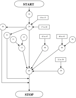
Fig. 9: Flowchart showing interaction of various functions used in the program.
3. An interactive session with ProEx-Cold
To show the functionality of ProEx-cold, few case studies are taken to illustrate process. 3.1.Interactive session for Non re-entry component shape
A square non re-entry shape as shown in Fig. 10 (zoom factor as 1.0) is taken to demonstrate the interactive session with the ProEx-Cold. Based on the input data provided by a user, ProEx-Cold executes the process program and first screen appears like a DOS command prompt as shown in Fig. 11.
Based on the user input, following geometrical data files are also generated as: ‘data.p’, ‘arbitrary.p’, ‘origin.p’, and ‘origin_elements’. The files are further used in generating the die, the billet and analyzing the upper bound analysis. If the die selected for extrusion is 3rd order-streamlined and the billet material is Aluminum alloy (Al 2024)
and for 70% reduction, the generated die, the billet and the final product are all displayed as shown in Fig. 12 and Fig. 13 respectively. The corresponding process plan sheet is generated as shown in the Fig. 14.
START
16
29
31 30
49
STOP
17 to 28
44 13
12 11
14 to 15
48
45 to 47 40 to 43
39 32 to 38
.
Fig. 10: Non re-entry cross-section geometry drew using AutoCAD
3.2.Interactive session for Re-entry component shape
A re-entry shape as shown in Fig. 15 (zoom factor as 1.0) is taken to demonstrate the interactive session with ProEx-Cold. On executing the program, the first screen looks like a DOS command prompt as shown in Fig. 16, based on the input data as provided by a user. Based on the input, the following geometrical data files are generated for the given re-entry shape as: ‘data.p’, ‘arbitrary.p’, ‘origin.p’, and ‘origin_elements’.
Fig. 15: I-section (re-entry) 2D geometry drew using AutoCAD.
The process of conversion from a re-entry shape to non re-entry shapes is carried by the following data files. - “data.p” file
- “arbitrary.p” file corresponding to whole geometry - “origin.p” file
- “origin_elements” file - “data1.p” file
- “arbitrary_elements_for_data1.p” file corresponding - “origin_elements_for_data1.p” file to first proposed - “origin_reentry_elements_for_data1.p” file non re-entry shape - “data2.p” file
- “arbitrary_elements_for_data2.p” file corresponding - “origin_elements_for_data2.p” file to second proposed - “origin_reentry_elements_for_data2.p” file non re-entry shape
The files corresponding to the geometry is used for generating the die, the billet. The files corresponding to proposed non re-entry shapes are used in analyzing the upper bound analysis. If the die selected for extrusion is 3rd
order-streamlined and the billet material is Aluminum alloy (Al 2024) then for a 60% reduction, the generated die, the billet and the final product are all displayed as shown in Fig. 17 and Fig. 18 respectively. The corresponding process plan sheet is generated as shown in the Fig. 19.
4. Conclusions
The user-friendly CAPP system ProEx-Cold is developed for cold extrusion of solid extrudable components capable of optimizing the die length and its display for non re-entry as well as re-entry component shapes. The CAPP system generates 3D colored drawing simulating the extrusion process. Animation helps to check the movements of billet before entering the die and to the final extrudate out of the die. The present CAPP system is capable of generating the optimal process plans and can also be used as a tool for parametric study.
The parametric study shows that the average ram pressure increases almost linearly with friction factor. It increases up to 60% reduction & increases sharply above 60% reduction. It is minimum corresponding to optimal die length that decreases with increase in the fiction factor. On basis of power minimization criterion, the 3rd order streamlined die is
found to be the best amongst various extrusion dies. It is interesting to note that the ProEx-cold work can be extended for hollow extrusion and multi-hole extrusion as well as for hot extrusion cases.
x-Cold (non re-entry shape).
Acknowledgements
The financial support of Department of Science & Technology (India) [Grant nos. III .5(109) /2001- SERC (Engg) dated 19.02.2002 and SR/S3/MERC-07/2005 dated 12.05.06] is gratefully acknowledged.
References
[1] Kumar, S.;( 1999). A generative Interactive and Feature based Computer Aided Process Planning System for Cold Extrusion, Ph. D. Thesis, Indian Institute of Technology, Kanpur.
[2] Altan,T; Gunasekera , J.S.; Gegel , H.L.;. Malas,J.C; Morgan, J.T. (1982).ComputerAided Process Modelling of Hot Forging and Extrusion of Aluminum Alloys, CIRP Annals, 31,pp. 131-152.
[3] Dong, X; Devries,W.R; M. J. Wozny,M.J.;(1991). Feature based reasoning in Fixture Design, Annals of CIRP,(40-1), pp.111-114.
[4] Lanka, K.;(1998). Some a roaches to Automatic Recognition of Machining Features from 2D CAD Models, Ph.D. Thesis, Mechanical Engineering Dept., REC-Warangal (AP) India.
[5] Yeo, Swee-hock.;(1994). Knowledge-based feature recognition for machining, Computer Integrated Manufacturing Systems.(7-1), pp.29-37.
[6] Liu, Chia Hwa.; Perng, D.B.; Chen,Z.;(1995). Automatic form feature recognition and part reconstruction from 2D CAD drawing, Computers in Engineering, (25-4), pp.689-671.
[7] Ganter,M.A.; Skoglund, P.A.;(1993). Feature Extraction for Casting and Core Development, Trans. ASME, Journal of Pattern Recognition 115, pp.744-757.
[8] Milacic, R.V.; SAPT-expert system for manufacturing process planning, Computer Aided Intelligent Process Planning, edited by Liv, C. R.; Chang. T. S.; Konduri, R.;(1985). (ASME Winter Annual meeting .
[9] Raggenbass, A.; Reissener,J.; Automatic generation of NC Production plans in stamping and laser cutting, Annals of CIRP (1991),(40-1), pp.247-250.
[10]The Official Guide to Learning OpenGL, Version 1.1, OpenGL Programming Guide (1997). Addison-Wesley Publishing Company-Second Edition.
[11] Link, C.H.; CAPP - CAM-I Automated Process Planning System (1976). Proceedings of the 13th Numerical Control Society Annual Meeting
and Technical conference, Cincinnati, Ohio.
[12]Tulkoff, J.; Lockheed’s GENPLAN(1981)., 18th Numerical Control Society Annual Meeting and Technical conference, Dallas, Texas, pp.417.
[13]Chingping, Li. J. Han; Ham, I.;CORE–CAPP – A Company Oriented Semi-generative Computer Automated Process Planning System(1987), 19th International Conference on Manufacturing Laboratory Systems, Pennsylvania State University.
[14]Wyask, R. A.; An Automated Process Planning and Selection Program: APPAS(1977), Ph.D.Thesis, Purde University, West Lafayette, Indiana. [15]Kotler, R. A. ; Computerized Process Planning – Part 1 and 2(1980). Army Man Tech Journal, 4,(4- 5).
[16]Kumar, S.; Shanker, K.; Lal, G. K. A Feature Recognition Methodology for Extrudable Product Shapes(1999). International Journal of Prod. Res. (37- 11), pp.2519-2544.
[17] Gunasekhera, J. S.; CAD/CAM of dies(1989). Ellis Horwood Limited, U. K.
[18]Kumar, S.; Shanker, K.; Lal, G.K.; A Generative Process Planning System for cold Extrusion(2003). International Journal of Prod. Res. (41-2), pp.269-295.
[19]Kumar, Rahul.; 3D Generation of Extrusion processes and CAPP(2005), unpublished M.Tech. Thesis, Institute of Technology – Varanasi (India).
[20]Kumar, S.; Shanker , K.;. Lal, G.K.; Analysis of Cold Extrusion of Non Re-entry product Shapes(2002). Journal of Manufacturing Science and Engineering,124, pp.71-78.
![Fig. 3: Segmentation of re-entry shape into proposed non re-entry shapes [3].](https://thumb-us.123doks.com/thumbv2/123dok_us/9628800.1490901/5.612.109.464.96.228/fig-segmentation-entry-shape-proposed-non-entry-shapes.webp)
![Fig. 7: Relationship between die surface and projected surface [Santosh et. al. 2003]](https://thumb-us.123doks.com/thumbv2/123dok_us/9628800.1490901/15.612.157.481.84.299/fig-relationship-die-surface-projected-surface-santosh-et.webp)