IDENTIFYING STATIONARY PERIODS AND DISTRIBUTION SELECTION FOR QUEUEING PROCESS

(1)

ISSN 2320-9186

www.globalscientificjournal.com

GSJ: Volume 7, Issue 5, May 2019, Online: ISSN 2320-9186

www.globalscientificjournal.com

I

DENTIFYING

S

TATIONARY

P

ERIODS AND

D

ISTRIBUTION

S

ELECTION FOR

Q

UEUEING

P

ROCESS

Oke, J. A.

FEDERAL SCHOOL OF STATISTICS, IBADAN, OYO STATE, Nigeria. [email protected]

KeyWords

queueing process, test for stationarity, test for invariance, distribution selection.

ABSTRACT

The study adopted a systematic plan to observe and record the events of customer arrivals (C(t)), interarrival times (It) and

service times (St). The observations were recorded hourly at different periods (morning, afternoon and evening) daily in a

week at Nigerian National Petroleum Corporation (NNPC) Mega Station Port Harcourt Enugu Express, Emene, Enugu. Stationary periods were identified by considering two adjacent time intervals (0, t1) and (t1, t2), the invariance of It and St

were checked for the different periods. Test of stationarity and invariance were tested with non parametric tests of Mann-Whitney-Wilcoxon, and Friedman Two-way ANOVA respectively, which found stable for all periods. The It and St fitted

exponential distribution in all the periods through the Anderson Dalling test of goodness of fit. At the stationary periods, the most suitable fitted exponential distribution for It and St were selected respectively for the distribution of the queue

(2)

ISSN 2320-9186

INTRODUCTION

Queues are phenomena of everyday life. Human and non human wait in queues, students wait at bus stands to enter school bus; they wait at banks to pay school fees; vehicles wait at filling stations to buy fuel; customers wait at mall to obtain food items; they wait in front of point of sale terminals to pay for the items bought; etc. Queueing theory is the study of waiting in various guises (Frederick and Gerald, 2001). It uses queueing models to represent the various types of queueing systems (systems that involve traffic or queues of some kind) that arise in practice. Queueing theory is defined as the development of mathematical models to describe various types of queueing systems so that it may be possible to predict how the system will perform in a given demand situation Eze et al (2005). There are basic elements responsible for queueing, they are: input process; service mechanism; system capacity; and queueing discipline. According to Bhat (2008), the nomenclature for symbolical representation of the traffic system with ranges of system elements are recognized by these basics. Input/service/number of server is the three elements symbol mostly adopted for representations in queueing theory, although there are six symbols in the general specification of queueing which is known as Kendal’s notation (I/S/s/b/P/Sd). The I specifies inter-arrival time distribution, S specifies service time distribution, s specifies number of servers, b specifies number of buffer (the system capacity), P specifies population size and Sd specifies service discipline. The inter-arrival and service time distributions (i.e. I/S of the Kendal’s notation above) can be fitted any of exponential (M), Erlang with parameter k (Ek), hyperexponential with parameter k (Hk), deterministic (D), or general i.e. any distribution (G).

Consequently, if we have queueing system with infinite buffer capacity, infinite population size and service discipline is First Come First Serve (FCFS), the b/P/Sd is omitted in the Kendal’s notation above and thereby resulted to the three elements symbol I/S/s only. For example, we can have M/M/1 (the two Ms are exponential inter-arrival and service time distributions with 1 server) or M/G/1 (M exponential inter-arrival and G general service time distribution with 1 server) or M/M/s (Ms exponential inter-arrival and service time distribution with s servers).

In building a suitable probability model for queue system, we start with its elements. Of the four elements mentioned earlier, number of servers, system capacity and discipline are normally deterministic (unless, the number of available servers becomes a random variable). But there are uncertainty related to arrivals and service process which result in the underlying process being stochastic. The similarity of arrival and service processes can be brought out by identifying similar components, such as inter-arrival times and service times. Therefore, the possibilities of using certain probability distributions to represent the process of inter-arrival times and service times are main concern of any queueing study.

There are types of queue; Single Queue with Single Service Point; Single Queue with Multiple Service Points; Multiple Queues with Multiple Service Points; and Multiple Queues with Single Service Point. In this study, Single Queue with Multiple Service Points where one waiting line is formed but there are several servers was adopted, each server capable of meeting the demand of individual in the queue.

Ger and Avishai (2001) in their work raised issues with queueing models, they argued that most work on queueing lack practical solution. They discouraged comparison between analytical models and simulation model. The relevance of appropriate method of data collection and analysis for such system performance was pointed out. They warned that assumed stationarity could be problematic if the system does not relax fast enough. It was opined that system performance can only be tracked if system of queue is study over a short interval of time and study in peak period should be avoided for it is extremely sensitive to changes in its underlying parameters.

In order to contribute to the existing studies, this work focus on identification of stationary periods which were problem found in most queueing works which are deemed necessary before assuming M/M/S queueing. Fredrick and Gerald (2001), Ger and Avishai (2001), and Bhat (2008) emphasized that this is the only period where probability distribution can be assumed.

The crucial intention of the investigation of queueing systems as described by Bhat (2008) is to comprehend the manners of their fundamental processes and able to give conversant and sharp decisions in their administration. Among other concerned problems of studying queueing system which face most researchers were the steady state or stationary period and how can the period be identified? Let X(t) be a markov chain and number of customers at time t in a queueing system. If the system was observed for a very short interval of time h from time t, the probability X(t) in (t, t+h) is Pn(t+h).

According to Mitrofanova (2007), the probability that there will be an increase of size 1 when h is short and h → 0 is P(X(t + h) – X(t) = 1| X(t) = n) = λnh + o(h); P(X(t + h) – X(t) = -1| X(t) = n) = µnh + o(h) when the system decrease by size 1, and P(X(t + h) – X(t) =

0| X(t) = n) = 1 – (λn + µn)h + o(h) for the probability that more than one event will occur. The λn and µn are birth and death rate

(3)

ISSN 2320-9186

Using Kolmogorov forward equation for the birth and death processes;

(

)

3 (t) P μ (t) P λ (t) )P μ (λ (t) P h (t) P h) (t P Lim 2 h o(h) (t) P μ (t) P λ (t) )P μ (λ h (t) P h) (t P 1 o(h) (t) hP μ (t) hP λ (t) )hP μ (λ (t) P (h) (t)P P h t P 1 n 1 n 1 n 1 n n n n n n n 0 h 1 n 1 n 1 n 1 n n n n n n 1 n 1 n 1 n 1 n n n n n 0 k k n n + + − − → + + − − + + − − ∞ = − + + + − = ′ = − + ⇒ + + + + − = − + ⇒ + + + + − = = +

∑

k

Equation (3) is the differential equation for the birth and death process.

In the study of queue, we consider only stationary system (i.e. system of equilibrium). That is when Pn(t) = Pn

Equation (3) becomes;

(

λ μ

)

P λ P μ P 4 0=− n + n n + n−1 n−1 + n+1 n+1

For M/M/S











>

=













−

≤

=













=













=

∴

>

=

≤

=

− −

5 s

n

P

s

s!

γ

P

(s

μs

μ

s!

λ

P

μ

1)

μ)μ.sμ..

μ...(s

λ

s

n

P

n!

γ

P

μ

λ

n!

1 P

μ

n!

λ

P

μ.2μ....nμ

λ

P

s

n

s

μ

s

n

μ

λ

0 s n n 0 s n s n 0 n 0 n 0 n 0 n n 0 n n n n n

Consequently, the objective of this study is to identify the stationary periods, test the stationarity of the queueing process and fit theoretical probability distributions into interarrival time It and service time St at the stationary periods.

Material and Method

The data used for this study was a primary data collected from customers who bought Premium Motor Spirit (PMS) called petrol using direct observation method for three periods of the day i.e. morning, afternoon and evening for one week at NNPC Mega station Enugu-Port Harcourt express way, Emene, Enugu.

The NNPC Enugu Mega Station opens at 6 AM in the morning and closes at 6 PM in the evening. Therefore, a systematic collection of hourly observations was adopted. These hours were: 8.30 – 9.30 AM (morning); 12.30 – 1.30 PM (afternoon) and 4.30 – 5.30 PM (evening) With this, 21 periods’ observations were recorded in seven days. The station has two gates, one for entrance and the other for exit. The service capacity for PMS (petrol) in the station is 12 pumps (servers). These 12 pumps are arranged in parallel of three (3) lines. A line contains two (2) machines with two (2) pumps each. Customers form queue along the road leading to the entrance gate.

In order to get the system elements, a traffic form was designed to capture: C(t) = number of customers in one minute

At = customer arrival time

It= interarrival time (i.e. At – At-1)

Et = entry to service time

Dt = departure time

(4)

ISSN 2320-9186

The number of arrivals from two adjacent time intervals (0, t1) and (t1, t2) was observed for several time periods. Let X1, X2, …, Xn be

the number of arrivals during the first interval for n periods, and let Y1, Y2, …, Ym be the second interval for m periods (usually m =

n). In line with Conover (1971) and Randle and Wolfe (1979), the stationarity of the queueing process was tested with Mann-Whitney-Wilcoxon test on the observed arrivals from the two intervals. If F and G represent the distributions of the X’s and Y’s, respectively, then the hypothesis to be tested is F = G against the alternative F ≠ G, for which the Mann-Whitney-Wilcoxon statistic can be used. The Mann-Whitney-Wilcoxon statistic was defined by Hogg and Craig (1970) as

Zu =

12 1) n mn(m

2 mn U

+ + −

(for n or m > 20) 6

under the null hypothesis F(z) = G(z) and decision rule that: if the p value for the test statistic (Zu) is greater than 0.05 (level of

significance) accept H0 otherwise reject.

where

2 1)

n(n

T

U

=

−

+

If we pooled X1, X2, …, Xn and Y1, Y2 …, Ym together, we will get m + n items. T is the sum of the ranks of X1, X2, …, Xn among the

m + n items X1, X2, …, Xn, Y1, … , Ym-1, Ym, once the combined sample has been ordered.

To test the invariance of the system variables, we adopted the nonparametric technique of Friedman Two-Way Analysis of Variance by Ranks because of the skewed distributions of interarrival times and service times (Frederick and Gerald, 2001). Also there are two factors, the first is the periods and the other is the days.

For the Friedman test, the data were casted in a two-way table having 3 rows and 7 columns. The rows represent periods of the day (i.e. morning, afternoon and evening), and the columns represent the days of the week (i.e. Monday, Tuesday, …, Sunday). In as much as the columns contain equal number of cases, an equivalent statement would be that under H0 the mean ranks of various columns

would be about equal and decision is taken base on decision rule that: if the p value for the test statistic is greater than 0.05 (level of significance) accept H0 otherwise reject. The Friedman test determines whether the rank totals (Rj) differ significantly. To make this

test, we compute the value of a statistic which Friedman denotes as

χ

_r2. It can be shown that

χ

_r2 is distributed approximately as Chi square with df = k – 1 (Siegel, 1956), when

1)

3N(k

R

1)

Nk(k

12 χ

k

1 j

2 j 2

r

=

₊

∑

−

+

=

7

where N = number of rows; k = number of columns; Rj = sum of ranks in jth column.

In order to identify the distribution of a given data, Minitab (a statistical package) can be used to identify distribution any given data using the following procedure (Frost, 2012):

Stat>Quality Tools>Individual Distribution Identification (in Minitab)

This handy tool easily compares how well one data fit 16 different distributions. It produces a lot of output both in the Session window and graphs (Frost, 2012). It was explained further that there were measures to check in the output.

Anderson-Darling statistic (AD): lower AD values indicate a better fit. It is generally valid to compare AD values between distributions and go with the lowest

P-value: One needs a high p-value. A low p-value (e.g., < 0.05) indicates that the data do not follow that distribution.

The A-D statistic controls the hypothesis that the sample derives from a distribution which is described by the fitted density function, using the A2_statistic:

A2_{= N – S} ₈

where

∑

[

( )

(

)

]

= +−

−

+

−

=

N

1 i

i 1 N

i

In

1 F

x

InF

N

1 2i

S

and x1, …, xN are the sample values sorted in order of magnitude. Gavriil et al

(5)

ISSN 2320-9186

The presentations and computations in the next section will be facilitated using the following spreadsheet packages: Ms Excel, SPSS and Minitab.

ANALYSIS AND RESULT

The third-ten minutes of the 21 periods (morning, afternoon and evening for seven days of the week) were considered and data for the test were obtained within two adjacent time intervals (t0 = 0, t1 = 5mins] and (t1 = 5mins, t2 = 10mins]. Hence, number of arrivals in

between A(t0) and A(t1) is C(ti) (Xi for easy transcription) and number of arrivals in between A(t1) and A(t2) is C(tj) (Yj for easy

transcription).

We mean, A(t1) – A(t0) = C(ti) = Xi i = 1, 2, …, n

A(t2) – A(t1) = C(tj) = Yj j = 1, 2, …, m

n = m = 21 The observed values for X’s and Y’s are displayed in table 3.1 below.

Table 3.1: Observed Number of Arrivals at [t0, t1] and [t1, t2]

S/N X Y

1 5 18

2 12 8

3 6 4

4 6 5

5 16 6

6 8 11

7 17 13

8 8 13

9 13 6

10 9 3

11 15 17

12 9 6

13 10 10

14 16 12

15 11 7

16 9 9

17 6 13

18 4 6

19 2 12

20 12 7

21 9 13

Using Mann-Whitney-Wilcoxon test, the result of the test by SPSS is displayed in Table 3.2 below.

H0: F = G

H1: F ≠ G

Decision rule: reject H0 if p value for Mann-Whitney-Wilcoxon test statistics is less than α = 0.05, otherwise accept.

Table 3.2: Mann-Whitney-Wilcoxon Test Statistics

Statistics C(t)

Mann-Whitney U 215.500

Wilcoxon W 446.500

Z -.126

(6)

ISSN 2320-9186

Under the null hypothesis (H0) that F = G, we would accept the H0 and conclude that the process is stationary at the two adjacent time

intervals considered as p-value (0.899) is greater than

α

=

0 .

05

. It is at this interval of times that we will determine our distributions for It and St.

From above, it is evident that the system is at stationary at the third-ten minutes of the periods. We took equal sample of size 20 at these periods and computed mean for It and St.

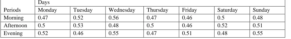
Putting the means of It in periods (rows) and days (columns), we have

Table 3.3: Means of It in periods and Days

Periods

Days

Monday Tuesday Wednesday Thursday Friday Saturday Sunday

Morning 0.47 0.52 0.56 0.47 0.46 0.5 0.48

Afternoon 0.5 0.53 0.48 0.5 0.46 0.52 0.51

Evening 0.52 0.46 0.55 0.47 0.51 0.48 0.55

H0: there is no significant difference in the means of It at the station during periods of days in a week

H1: there is significant difference in the means of It at the station during periods of days in a week

Decision rule: reject H0if p value for Friedman’s test statistics is less than α = 0.05, otherwise accept.

Table 3.4: Result of Friedman Test on Means of It

Test Statistics

N 3

Chi-Square 6.218

Df 6

p-value. .399

Putting the means of St in periods (rows) and days (columns), we have

Table 3.5: Means of St in periods and Days

Periods

Days

Monday Tuesday Wednesday Thursday Friday Saturday Sunday

Morning 2.53 2.56 2.65 2.45 2.45 2.46 2.52

Afternoon 2.53 2.47 2.47 2.42 2.53 2.53 2.47

Evening 2.44 2.53 2.50 2.59 2.52 2.55 2.45

Test of hypothesis

H0: there is no significant difference in the means of St at the station during periods of days in a week

H1: there is significant difference in the means of St at the station during periods of days in a week

Decision rule: reject H0if p value for Friedman’s test statistics is less than α = 0.05, otherwise accept.

Table 3.6: Result of Friedman Test on Means of St

Test Statistics

N 3

Chi-Square 2.226

Df 6

p-value .898

The two results show that the means of Yt and St are invariant over the days of the week and times of the day at the stationary periods.

It implies that the events Yt and St remain the same at some interval of times from Monday to Sunday and any period of the days (in

(7)

ISSN 2320-9186

The distributions of Yt and St at stationary periods were fitted exponential distribution and tested for goodness-of-fit.

Anderson-Darling goodness-of-fit was tested on the fitted distributions and the results are presented below. Table 3.7: Test of goodness of fit result

Day Period

It St

MLE Scale (mean)

AD

statistic P value

MLE Scale (mean)

AD

statistic P value

Mon

Morning 0.465 0.763 0.217 2.534 0.757 0.221

Afternoon 0.503 1.129 0.077 2.531 1.233 0.058

Evening 0.518 1.052 0.095 2.438 1.275 0.052

Tue

Morning 0.521 1.254 0.055 2.556 1.217 0.061

Afternoon 0.531 0.876 0.155 2.467 1.261 0.054

Evening 0.461 1.162 0.07 2.534 0.757 0.221

Wed

Morning 0.56 0.71 0.254 2.651 1.209 0.062

Afternoon 0.478 1.218 0.06 2.467 1.261 0.054

Evening 0.545 1.272 0.052 2.498 1.209 0.062

Thu

Morning 0.465 0.763 0.217 2.445 1.176 0.068

Afternoon 0.503 1.29 0.077 2.418 0.854 0.166

Evening 0.467 1.129 0.077 2.589 0.777 0.208

Fri

Morning 0.461 1.162 0.070 2.445 1.176 0.068

Afternoon 0.455 0.561* _0.400* _2.534 _0.757 _0.221

Evening 0.513 1.19 0.065 2.518 0.669* _0.288*

Sat

Morning 0.503 1.129 0.077 2.462 1.112 0.081

Afternoon 0.518 0.85 0.168 2.534 0.757 0.221

Evening 0.475 0.816 0.185 2.55 0.81 0.189

Sun

Morning 0.475 0.816 0.185 2.517 1.171 0.068

Afternoon 0.513 1.19 0.065 2.467 1.261 0.054

Evening 0.549 0.887 0.151 2.445 1.176 0.068 *lowest AD statistic with highest p value

In the above table, It and St fitted exponential distribution for all days and periods during the stationary periods since all p values are

greater than 0.05 for all AD statistic. The most fitted exponential distribution is the one with lowest AD value and highest p value (0.561 and 0.400 for It; 0.669 and 0.288 for St). Therefore, the distribution selection for It and St was exponential distribution with

parameter scale 0.455 and 2.518 respectively.

Conclusion

This work sought to find stationary periods for a queueing system as one of the assumption of m/m/s queueing model and fitted suitable distribution for the main stochastic elements (the interarrival (It) and service times (St)) of the model at the identified

stationary periods. Two adjacent times were observed for the periods and Mann-Whitney-Wilcoxon test was used to test the stationarity. The result shows that process is stationary with Mann-Whitney-Wilcoxon statistic, Z = -0.126 and p-value = 0.899. With the result, the hypothetical periods were confirmed stationary for the queueing model. Also, Friedman two-way ANOVA proved that the system variables were invariant with respect to days of the week and periods of the day. The results revealed that chi square statistics of Friedman with the p values for Yt and St were 6.218 (p = 0.399) and 2.226 (p = 0.898) repectively.

At the stationary periods, all Yt and St were fitted exponential distribution through Anderson-Darling (AD) goodness-of-fit for

continuous distributions. It was found that the most suitable exponential distribution for Yt and St was that with AD statistics 0.561,

(8)

ISSN 2320-9186

arrive for service in one minute with interarrival times averagely 0.5 minute and each customer’s service time is averagely 2.5 minutes.

It is recommended that strict adherence should be given to stationarity in the analysis of queueing study of m/m/s. This will give traceable and brilliant estimate of the system metrics.

References

Bhat, U. N. (2008). An Introduction to Queueing Theory, Springer Science Business Media, LLC, New York. Conover, W. J. (1971). Practical Nonparametric Statistics, John Wiley and Sons, New York.

Eze, J. I., Obiegbu, M. E. and Jude-Eze, E. N. (2005). Statistics and Quantitative Methods for Construction and Business Manager,YUM-SEG Enterprises, Lagos. Fredrick, H. S. and Gerald, L. J. (2001). Introduction to Operations Research, McGraw-Hill Higher Education, 7th_{edition, New York.}

Frost, J. (2012). “How to identify the Distribution of your Data using Minitab”, The Minitab Blog: Adventures in Statistics. :http://blog.minitab.com/blog/adventures-in-statistics/how-to-identify

Gavriil, I., Grivas, G., Kassomenos, P. and A. and Spyrellis, N. (2006). “An Application of Theoretical Probability Distributions to the Study of PM10 and PM2.5 Time

Series in Athens, Greece”, Global Nest Journal, vol. 8, No. 3.

Ger, K. and Avishai, M. (2001). Queueing Models of Call Centres, An Introduction, available at www.cs.vu.nl/obp/callcentres

Hogg, R. V. and Craig, A. T. (1970). Introduction to Mathematical Statistics, Macmillan Publishing Co, Inc, New York.