A novel method for 2D-to-3D video conversion based on boundary information

R E S E A R C H

Open Access

A novel method for 2D-to-3D video

conversion based on boundary information

Tsung-Han Tsai

, Tai-Wei Huang and Rui-Zhi Wang

Abstract

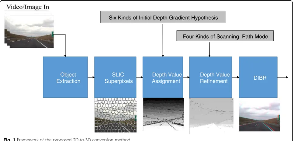
This paper proposes a novel method for 2D-to-3D video conversion, based on boundary information to automatically generate the depth map. First, we use the Gaussian model to detect foreground objects and then separate the foreground and background. Second, we employ the superpixel algorithm to find the edge information. According to the superpixels, we will assign corresponding hierarchical depth value to initial depth map. From the result of depth value assignment, we detect the edges by Sobel edge detection with two thresholds to strengthen edge information. To identify the boundary pixels, we use a thinning algorithm to modify edge detection. Following these results, we assign the depth value of foreground to refine it. We use four kinds of scanning path for the entire image to create a more accurate depth map. After that, we have the final depth map. Finally, we utilize depth image-based rendering (DIBR) to synthesize left and right view images. After combining the depth map and the original 2D video, a vivid 3D video is produced.

Keywords:3D video, 2D to 3D conversion, Depth map, Foreground segmentation, Superpixel, DIBR

1 Introduction

In the field of visual processing, 3D image processing has become very popular in recent years. To produce a better display than the traditional 2D visual experience, 3D displays offer a number of new applications, includ-ing education, games, movies, cameras, etc., with 3D video generations still growing. The user only watches 3D animation or 3D movies made by a special camera on a computer. The lack of 3D videos makes 2D-to-3D image conversion quite practical.

Synthesis technology from a 2D image to a 3D image is performed in two steps: an estimation of the original 2D image depth map and then taking advantage of this depth map to synthesize a 3D stereoscopic image. Thus, the quality of the depth map largely affects the quality of the 3D image. According to whether human interven-tion, we can divide 2D to 3D image synthesis in two ways: automatic and semi-automatic [1]. In automatic methods, human-computer interactions are not in-volved. The process has different visual cues, ranging from motion information to perspective structures. In [2] they proposed a geometric and material-based

algorithm, but the major issue of a fully automatic method is creating a robust and stable solution for any general content. This brought about semi-automatic methods that contain some human-computer interac-tions to balance quality. The stereo quality and conver-sion cost are determined by key frame intervals and the accuracy of depth maps on key frames. Guttman et al. set up a semi-synthetic depth map method [3] with a sparse labeling depth estimation method. It handles depth with several key images for the semi-automatic method and uses others with an automatic synthesis to improve accuracy. Obviously, how to determine the key image influences the accuracy of the entire depth map.

Regardless of the algorithm being fully automatic or semi-automatic processing, a static scene with moving parts is one of the most common issues. To generate a depth map in this scenario, a static background is typic-ally a layer of depth values, deriving an accurate capture of mobile objects. In [1] they utilized motion estimation [4] to present a conversion which requires only a few user instructions on key frames and propagates the depth maps to non-key frames. Huang et al. used H.264 codec to encode the motion vectors and combined two kinds of depth cues: motion information and the geo-metric perspective [5]. Raza [6] presented a method for * Correspondence:[email protected]

Department of Electrical Engineering, National Central University, No.300, Jung-Da Rd., Jung-Li City 320, Taiwan, Republic of China

a dynamic scene. It needs several kinds of information to process, including object shape, movement amount, shield-ing geometry edges, and scene, to get depth information.

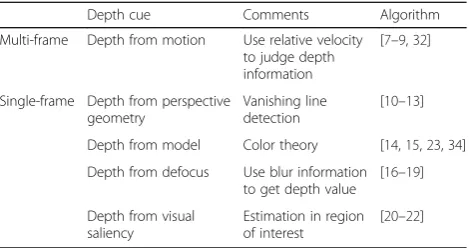
Since depth information is the most important issue for 2D-to-3D conversion, how to technically produce an accurate depth map is critical. Depth map generation can be classified into single-frame and multi-frame methods. Multi-frame methods are based on stereo/ multi-view with the related depth information. Depth from motion is realized by the information of relative velocity [7–9]. In [7], they used the depth from motion and solved a multi-frame structure from the motion prob-lem. The method uses the epipolar criterion to segment the features belonging to the independently moving objects. In [9], they applied a block-based method and cooperated with the bilateral filter to diminish the block effect and to generate a comfortable depth map.

Multi-frame methods are achieved based on high-cost equipment to acquire multiple video scenes. Conversely, a single-frame method is derived based on only one-view information with its depth information. Depth from

the perspective geometry has been used in [10–13].

These methods mostly took vanishing line detection to identify the depth information. Battiato [10] proposed a method based on the position of the lines and the van-ishing points to derive a suitable assignment of depth. In [12] they gave a semi-automatic method aimed to gener-ate stereoscopic views estimating depth information from a single input video frame and to decrease compu-tation resources. Depth from a model is also used to es-timate the depth value in [14, 15]. In [14] they approximated 3D structures of natural scenes to gener-ate stereo images, using warm or cool color theories to generate depth data with simple models. Some utilized the defocus method to extract depth information, as in

[16–19]. In [17] they employed blur information based

on the number of high-value coefficients by wavelet transform. Depth from visual saliency is also used to analyze visual attention and saliency in [20–22]. In [20] they set up a method based on visual saliency to extract the regions of interest from a color image. Additional methods have applied a combination of several depth cues to determine the depth information, such as in [3, 5, 6]. Jung et al. [23] proposed a depth-map estima-tion algorithm under the assumpestima-tion that the depth of image will increase from bottom region to upper re-gion. Table 1 lists the classification of the methods on depth map generation. Referring to the 3D image/ video generation techniques, depth image-based ren-dering (DIBR) is commonly used for 3D image/video generation [24]. Different from classical method which requires the two streams of video images [25], DIBR requires a single image and the second images usually are depth images. In addition, the depth maps can be

coded more efficiently than two streams of natural im-ages, thus reducing the bandwidth requirement.

In this work, we proposed a 2D-to-3D conversion method based on single-frame method and fully auto-matic conversion to generate stereo visual results. We use GMM (Gaussian mixture model) and SLIC (simple linear iterative clustering) to generate initial depth map and then utilize edge information and repeat four kinds of scanning path mode to refine the depth value. After-wards, we have a precise final depth map. By DIBR, we produce the left and right view images to complete 2D-to-3D conversion. This paper is organized as follows. Section 2 provides an overview of the proposed method. Section 3 describes the Gaussian mixture model. Section 4 discusses the technique on superpixels. Section 5 amends depth map generation. Section 6 provides the experi-mental results and discussion. Finally, a conclusion is given in Section 7.

2 Overview of the proposed method

The proposed method is based on two concepts: (1) the moving object is a part of the focus; (2) the object ap-proach to the bottom part of the screen should be close to the camera; on the contrary, the object should be far away from the camera. The second assumption applies in most cases, such as the works in [23, 26]. Taking these two concepts, we use foreground detection and super-pixel algorithms to extract the object information. Boundary information is the important result that we can manipulate. Several important characteristics are as follows.

1. Fully automatic conversion is contained;

2. Foreground detection and edge information help unify the depth value on the object;

3. Superpixel algorithm clusters pixels with close information;

4. Six kinds of initial gradient hypothesis for initial depth map;

Table 1The classification of the methods on depth map generation

Depth cue Comments Algorithm

Multi-frame Depth from motion Use relative velocity to judge depth information

[7–9,32]

Single-frame Depth from perspective geometry

Vanishing line detection

[10–13]

Depth from model Color theory [14,15,23,34]

Depth from defocus Use blur information to get depth value

[16–19]

Depth from visual saliency

Estimation in region of interest

5. Four kinds of scanning modes to fix the depth map;

6. Through a Hough transform, we only extract one-line information to get the slope of the line.

Figure 1 shows the structure of the proposed frame-work. The proposed 2D-to-3D conversion method in-cludes several major stages. First, the foreground segmentation stage segments foreground object and as-signs background initial depth values. The Gaussian model detects foreground objects. As a result, the de-tected foreground benefits the depth value refinement compared with the methods without foreground infor-mation. The superpixels stage clusters pixels and assigns depth values based on edge information. We employ this algorithm to refine the edge information. Pixels with similar color and position information are clustered. Edge information is then included to assign the same depth value. We utilize the Hough transform with six initial depth maps. According to the pixels clustered by superpixels, we give initial depth values. At the

in-depth value refinement stage, we apply four scan-ning modes to modify depth values and then apply Sobel edge detection with two-threshold decision to get different results of edge detection. To identify

the boundary’s pixel, we use a thinning algorithm to

the extracted edge so that only one pixel is presented on a boundary. Based on the derived depth map, two-view images are rendered by DIBR. Finally, we display it on a 3D displayer.

3 Gaussian mixture model

Foreground is defined as an object that has different mo-tion vectors relative to the most similar momo-tion vectors between each neighbor frames. Since the moving object is usually called the foreground, we determine the motion vector of the object to classify foreground and background, as shown in Fig. 2.

3.1 Background modeling

In our approach, the adaptive background subtraction method is based on moving object detection and

Depth Value

Assignment DIBR

Object Extraction

SLIC Superpixels

Depth Value Refinement

Six Kinds of Initial Depth Gradient Hypothesis

Four Kinds of Scanning Path Mode

Fig. 1Framework of the proposed 2D-to-3D conversion method

background modeling. The adaptive background subtrac-tion method uses the models as a mixture of Gaussians and an on-line approximation to update the models [17]. We employ Gaussian distribution to determine the back-ground and only use the luminance value of the YUV color space with frame shifting. When a pixel is at timet, it can be written asX ={X1,…,Xt}. This pixel is combined by the amount ofkGaussian distribution. The probability of observing the current pixel valueP(Xt) is shown in (1).

P Xð Þ ¼t

XK

i¼1wi;t _pðX

t;μi;t;Σi;tÞ ð1Þ

where K is the number of distributions, ωi,t is an esti-mate of the weight of theith Gaussian in the mixture at time t, μi,t is the mean value of the ith Gaussian in the mixture at timet,∑i,tis the covariance matrix of the ith Gaussian in the mixture at time t, and p is a Gaussian probability density function shown as:

P Xð t;μ;ΣÞ ¼

1 2π ð Þn

2j jΣ12

e−21ðXt−μtÞ T_Σ−1

Xt−μt

ð Þ ð2Þ

According to each Gaussian’s parameter, we can evalu-ate which is the most accurevalu-ate distribution of the

background. Based on the variance and the persistence of each mixture of Gaussians, we determine which Gaussians may correspond to the background colors. Be-cause there is a mixture model for every pixel in the image, we use [27] to execute our algorithm. Each new

pixel value Xt is checked with the existing K Gaussian

distributions until a match is found. A match is defined as a difference between a pixel value and mean within a

threshold of covariance. If one of the K distributions

matches the current pixel value, the parameters of the distribution are updated. When Gaussian distributions have greater weight and smaller variance, they are usu-ally identified as the background model. Figure 2 shows the results of the background model.

The update for Gaussian distribution is continuously performed on the matched and unmatched parts. As a result, the convergence issue dominates the speed and complexity. Based on (1, 2), we modify it as:

ρ¼αp

Xtjμk;t;jΣk;t

ð3Þ

ηk;t ¼_counterρ

k;tþ1þρ ð4Þ

where η(t) is a convergence factor. In traditional methods, this factor is set as a constant value or variable that decreases at constant time. This induces low con-verge speed or hard to concon-verge, respectively. Our modi-fication solves these issues.

3.2 Moving object detection

According to the background modeling, every Gaussian has a value of ω/σ, where σ is the covariance of distri-bution. When Gaussian distributions have a maximum

ω/σ, they become background modeling. Moving

S S

2S

Fig. 3Reducing search range on superpixels

a

b

objects can then be distinguished from the original 2D

image through theith Gaussian with the maximumω/σ

background model. We then binarize the moving object and background. For easy representation, the pixel of a moving object is assigned a white color, and its background is black. The determination is as follows:

A xð;yÞ ¼ 255; I xð ;yÞ−μk>T 0; I xð;yÞ−μk≤T

ð5Þ

whereA(x,y) is the binary result of moving objects’ de-tection, I(x, y) is the current pixel value of the image, andTdenotes a threshold. Figure2a, c shows the results of moving object detection.

4 SLIC superpixels

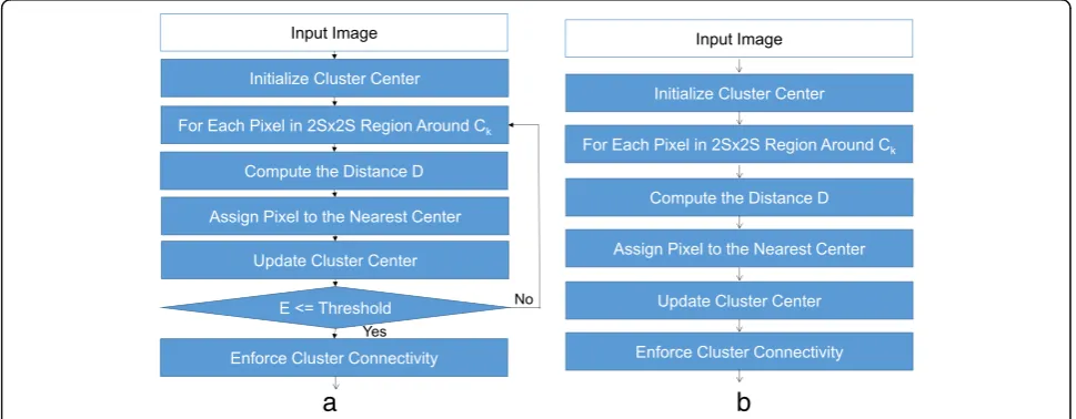
This section introduces SLIC superpixels. According to [28], using SLIC to generate superpixels is faster than other superpixel methods, i.e., normalized cuts algo-rithm. It exhibits state-of-art boundary adherence more efficiently and improves the performance of the segmen-tation algorithm. We further modify the SLIC method to speed up this process.

4.1 Concept of SLIC algorithm

Simple linear iterative clustering is an adaptation of

K-means for superpixel generation. The only

param-eter of the algorithm is k, which represents the

number of approximately equally sized superpixels. For color images, we transform color space from YUV to CIELAB. The clustering program begins with an initialization step where k initially clusters centers, called Ck. The clustering of grid size is S=√N/K,

where N is all the pixels of an image, and Ci = [li, ai,

bi, xi, yi]T is the color space for each pixel. The pixel

tag of an image is −1. The distance value D is

assigned as infinity.

Figure 3 illustrates the difference between the standard

and SLIC methods. The standardK-means method searches

the entire image by clustering the center. The complexity is

O(kNI), whereIis the number of iterations. Within 2Sx2S clustering center, SLIC is applied to search this limited re-gion. Thus, the complexity is reduced toO(N).

4.2 Distance measurement

This algorithm is used on CIELAB color space, where [l a b]T is the color space, and [x y]T is the location

information of the pixel. The distance value D helps

analyze the correlation among pixels and decides whether they can be classified as the same superpixels or not. We separate color information and location information to calculate them, shown in (6, 7).

dc¼

ffiffiffiffiffiffiffiffiffiffiffiffiffiffiffiffiffiffiffiffiffiffiffiffiffiffiffiffiffiffiffiffiffiffiffiffiffiffiffiffiffiffiffiffiffiffiffiffiffiffiffiffiffiffiffiffiffiffiffi lj−li

2

þ aj−ai

2

þ bj−bi

2

q

ð6Þ Fig. 5Using vanishing line to decide initial map

Input Image

Calculate Possible Feature Points

Find the Slope of Line

Which Initial Depth Map Be Used

Six Kinds of Initial Depth Gradient Hypothesis

ds¼

ffiffiffiffiffiffiffiffiffiffiffiffiffiffiffiffiffiffiffiffiffiffiffiffiffiffiffiffiffiffiffiffiffiffiffiffiffiffiffi xj−xi

2

þ y_j−y_i

2

r

ð7Þ

In order to calculate these two results, we use spatial distance coefficientNS and color space coefficientNCto

normalize the distance value. We can expressD’as:

D0 ¼

ffiffiffiffiffiffiffiffiffiffiffiffiffiffiffiffiffiffiffiffiffiffiffiffiffiffiffiffiffiffiffiffiffiffiffi dc

Nc

2

þ ds

Ns

2

s

ð8Þ

where S is the largest distance of the grid, and NC is a variety of coefficients according to different images or initialized grid. We apply a parameter m to control the tightness of the edge close to the image. Therefore, (8) is changed as follows:

D0 ¼

ffiffiffiffiffiffiffiffiffiffiffiffiffiffiffiffiffiffiffiffiffiffiffiffiffiffiffiffiffiffiffiffiffi dc

m

2

þ ds

s

2

s

ð9Þ

After the calculation on distance value D, the label of each pixel is updated. If the pixel has the smallest

distance value D with kth grid center, the label of the pixel will be updated by k. After each pixel has a corre-sponding label value, we average the color information and location with the same label value to get the grid’s new center. The process is repeated until convergence.

Searching always derives many times of iteration. Since this is very time-consuming, we need to consider its effi-ciency. Based on our several experiments, a one-iteration result is sufficient since there is almost no dif-ference compared with multiple-iteration results. Thus, we only execute a one-iteration result for SLIC in order to reduce processing time. Figure 4 shows the flowchart

of SLIC, and the parameter E in Fig. 4a means the

re-sidual error.

5 Depth extraction and depth fusion process

We employ edge information and superpixels to gener-ate depth map. After finding foreground, similar depth value is assigned to whole object by using edge infor-mation of the object in current frame. The extraction and fusion on the depth are the key technique for

Initial Depth Gradient Hypothesis

Width

Height

Slope Slope

Slope Height

Width Width

(a)

(b)

(c)

(d)

(e)

(f)

Fig. 7Six kinds of initial depth gradient hypothesis

synthesizing 3D visual quality. In our approach, we give the corresponding hierarchical depth map after the superpixel information. We then use Sobel edge detec-tion and a thinning algorithm to capture the objects. Fi-nally, we utilize four kinds of directions to scan the entire image and correct the depth value to obtain the full depth map.

5.1 Depth from prior hypothesis

In most conversion techniques, vanishing line detection is needed to determine the initial depth map. Traditional vanishing line detection can get the one vanishing point. This is accomplished by a Hough transform [9] with

some extracted lines. At least two detected lines are able to decide a vanishing point, as illustrated in Fig. 5. In our method, we do not use vanishing line detection. In-stead, with the processing of a Hough transform, we just extract one line of information to get the slope and points of the line. With the slope of the vanishing line, we can determine the initial depth map. Without the de-cision on vanishing point and the related two vanishing lines, this simplifies this process.

We take the slope of one line to define the initial depth map from six kinds of initial gradient hypoth-esis, as shown in Fig. 6. In [26], they used five kinds of initial gradient hypothesis to decide this. We add

Four kinds Scaning path

Current pixel

Compared pixel

[0][0]

[0][n]

[m][0]

[m][n]

Fig. 9Four kinds of scanning path

another situation to satisfy the scene of an indoor case. In this case, the depth map is always from the outside to inside scene. Here, we identify it more pre-cisely. Referring to the decision on initial value, [26] used a block-based method to approximate it. Since we have implemented SLIC on a cluster, we can easily decide it based on this information. Figure 7 shows the six kinds of initial gradient hypothesis.

After determining the hierarchical initial depth map from six kinds of initial gradient hypothesis, we cal-culate the depth value for each pixel. The six cases are labeled from (a) to (f ) as illustrated in Fig. 7. For case (a), the depth map is bottom-to-up and is calcu-lated as:

1. Depth¼White−i _HeightWhite

;where 1<slope or −1>slope; i¼f1;2;3…;heightg(10).

For cases (b) and (c), the depth map is left-to-right and right-to-left, respectively. It is calculated as:

2. Depth¼White−i_WidthWhite;where slope¼0; i¼f1;2;3…;widthg(11).

For cases (d) and (e), the depth map is from lower left to upper right and lower right to upper left, respectively. It is calculated as:

3. Deptht ¼White−i ffiffiffiffiffiffiffiffiffiffiffiffiffiffiffiffiffiffiffiffiffiffiffiffiWhite

Width2_þHeight2 p

Depth¼Depth_t−j

i ffiffiffiffiffiffiffiffiffiffiffiffiffiffiffiffiffiffiWhite Width2þHeight2 p

N 0 @

1

A_;

where 1>slope or−1<slope;j

¼f1;2;3…;heightg ð12Þ

where Depth is the value assigned to the depth value; Width is the width of the image; and Height is the height of the image. Based on our experiment results, since the bottom-to-up model is one of the most common modes in the real world, we assign the bottom-to-up mode as the default mode. Depth¼White−i _HeightWhite

:

5.2 Sobel edge detection

We use Sobel detection to acquire the edge informa-tion of an object. A 3 × 3 Sobel operator is defined to detect horizontal gradient Gx and vertical gradient Gy.

After deriving the gradients, we use (13) to make the weighted gradient Gz.

pixelð Þ ¼p 255; Gz≥threshold 0; Gz<threshold

;

whereGz¼

ffiffiffiffiffiffiffiffiffiffiffiffiffiffiffiffiffi G2_xþG2_y q

ð13Þ

We take a threshold to compare with the gradient

value of pixel P to decide the existence of an edge. To

present a good result, we propose a two-threshold method to implement this. By these two thresholds, we have two different edge data. The large threshold main-tains strong edge information and masks the noise on boundary pixels. The small threshold represents week edge information and thus maintains more noise infor-mation. Through this two-threshold mechanism, the re-sult is more precise than a single threshold solution.

Because the thickness on an edge is not unified, we exe-cute a thinning algorithm [29] to represent a one-pixel thickness on a contour. The benefits are eliminating edge noise and refining the depth map in the following process.

Figure 8 shows the example of thinning result. We itera-tively delete the boundary pixels of an object. From the re-lationship of each pixel, we can iteratively keep or delete the boundary pixels of an object, thus deriving a skeleton.

5.3 Depth refinement

After the above steps, we have the depth map that is generated by two different Sobel thresholds. We use four kinds of scanning modes to fix the depth map [30]. The scanning paths are listed as follows:

1. From the lower right to the upper left: if the pixel’s depth information is smaller than the right, it will be replaced by the right;

2. From the lower left to the upper right: if the pixel’s depth information is smaller than the left, it will be replaced by the left;

3. From the upper left to the lower right: if the pixel’s depth information is smaller than the upper, it will be replaced by the upper;

4. From the upper right to the lower left: if the pixel’s depth information is smaller than the lower, it will be replaced by the lower.

As shown in Fig. 9, we repeat the above four scanning modes until it self-stabilizes and compared the depth map with the other depth map in different thresholds. This evaluation eliminates the edge profile. We then use adjacent depth information to fill in an edge profile. Finally, we compare with the foreground information to get the completed depth map.

6 Experimental results and discussion

6.1 Simulation results

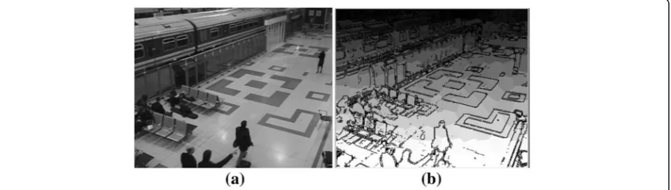
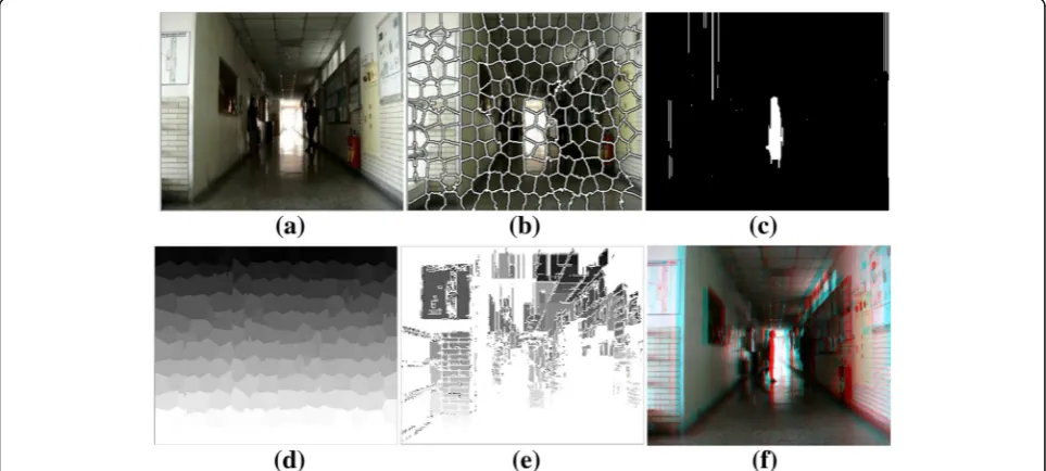
Figure 10 illustrates the experiment results with its detailed processing steps. First, the result by SLIC is shown in Fig. 10b. After the foreground detection, the object as foreground is extracted in Fig. 10c. Figure 11d–f shows the initial depth map, final depth map, and the ana-glyph image, respectively. We provide several simulation

results includingHall,Subway,Station,Hall monitor, La-boratory,Bridge close, andFlower. In brief, we only show the depth map result and the synthesized view as illustrated in Fig. 11.

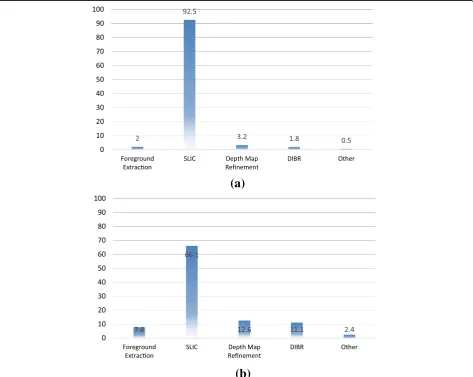
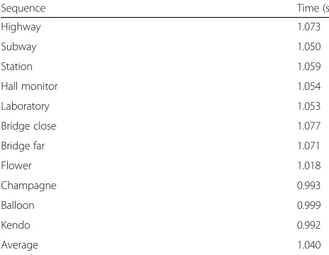
We implement our method on a workstation equipped with Intel 3.4GHz Core i7-3770 CPU and 8GB RAM. To evaluate the performance fairly, the entire algorithm is run with a single thread. Every test sequence is restricted to a 352 × 288 frame size. The profiling result is shown in Fig. 12 and Table 2 lists execution time of each sequence. Further-more, we profile it on PandaBoard platform, which is based on the Texas Instruments OMAP4430 system. As shown in Fig. 12, the average execution time is 1.040 s per frame in a PC environment and 4.13 s per frame on an embed-ded platform. SLIC occupies most of the computation time, no matter in the PC environment or embedded platform.

6.2 Evaluation and comparison

We evaluate and compare the visual quality of the pro-posed algorithm with the others. In comparison with the depth map of ground truth, our method easily reveals the stereo effect. From [31], they used their method to the videos and also provided the ground truth of video. We apply one of the videos, Kendo, as shown in Fig. 13. We pop out three frames in a video to express the con-tinuous result. Each frame of Fig. 13 shows the original image in the upper part. From the lower left to the right part, it shows the ground truth and the depth map by the proposed method, respectively. Since this video has high-motion characteristic, it is not easy to process well. It always induces some defects such as motion blurring, non-continuous depth, and uncomfortable feeling to viewers. Our method can perform this sequence as well as can be done in ground truth. Notably, the contour of sword is still clear even though movement arises. Table 2Execution time for each sequence (on PC environment)

Sequence Time (s)

Highway 1.073

Subway 1.050

Station 1.059

Hall monitor 1.054

Laboratory 1.053

Bridge close 1.077

Bridge far 1.071

Flower 1.018

Champagne 0.993

Balloon 0.999

Kendo 0.992

Average 1.040

Another simulation is made based on the ground truth in [6]. Three frames pop out as shown in Fig. 14. From the upper, the lower left, and the lower right, the images are the original, the ground truth, and proposed result, respectively. It shows that our method can gen-erate the depth map with a clear edge in objects, such as a car and a cloud. In comparison with ground truth, a cloud is ignored, but we are able to keep it well and make it easily protrude. A car should be treated as an object in Fig. 14. The ground truth is not very well dis-tinguishable. We can focus the car quite well with dif-ferent depth values around the neighbor. Three videos are also simulated and the results shown in Fig. 15, where the display order of each image is the same as in Figs. 13 and 14.

Because most reference works did not provide their simulated video sequences, we evaluate them by charac-teristics. Kim et al. [32] used motion analysis which cal-culated three cues that were used to decide the scale factor of motion-to-disparity conversion. However, it is hard to detect blending between shots. Li et al. [33] used

several simple monocular cues to estimate disparity maps and confidence maps of low spatial and temporal resolution in real-time, but it is less sensitive to the variety of scenes. In [34], it proposed a simplified algo-rithm that learns the scene depth from a large repository of image depth pairs. It can provide high performance but takes much computation time. In comparison with [26], they performed edge information to segment the objects. A similar work [30] also used edge detection and scan path to fill the depth values. If only the edge information is used, then it induces a same object with a different depth value. In our method, we not only use edge information, but also foreground detection to unify the depth value within the same object. Furthermore, two-threshold decision benefits the result on precise edge information and also avoids the disconnected result on an object and its depth value. Referring to [6], they learned and inferred depth values from motion, scene geometry, appearance, and occlusion boundaries. Al-though this can segment the images into spatio-temporal super-voxels and predict depth values with random forest Fig. 14Comparisons of depth map for Sequence_1 in [6].a. Frame 85.bFrame 93.cFrame 94. Images from upper, left to right are original images, ground truth, and depth maps of the proposed method

regression, it is still hard to segment an object from the background well.

From the depth map in Figs. 13 to 15, we provide the quantitative evaluation result. The performance of the generated stereoscopic video was evaluated sub-jectively by comparing a ground truth of a video se-quence. It was performed by 14 individuals with visual and stereo acuity. The participants watched the stereoscopic videos in random order and were asked to rate each video with depth quality. The overall depth quality was assessed using a five-segment scale, as shown in Fig. 16.

7 Conclusions

This paper has proposed a 2D-to-3D conversion algorithm. First, we separate the foreground and back-ground. Second, we use the superpixel edge algorithm to get boundary information and gather the pixels with the same depth value. Through a six gradient hypothesis on the depth map, the initial depth value is assigned. Since the boundary information is needed for refinement, we perform Sobel edge detection with two different thresh-olds to get two kinds of results. We then apply a thin-ning algorithm to obtain the result with only one pixel on edge. Compared with the two-threshold decision, we are able to add foreground information to unify the final depth information. Four scanning paths are used to re-fine the depth values. Finally, depth image-based render-ing is employed to synthesize a virtual image. In the future work, we will utilize more information such as visual saliency or use blur information to determine the initial depth map to deal with depth map in complex scenes more precisely.

Acknowledgements

This research was supported and funded by the Ministry of Science and Technology, Taiwan, under Grant 104-2220-E-008-001.

Authors’contributions

THT carried out the algorithm studies and participated in its simulation and drafted the manuscript. TWH designed the proposed algorithm. RZW help to execute the experiments. All of the authors read and approved the final manuscript.

Competing interests

The authors declare that they have no competing interests.

Publisher’s Note

Springer Nature remains neutral with regard to jurisdictional claims in published maps and institutional affiliations.

Received: 11 May 2017 Accepted: 3 December 2017

References

1. Z Li, X Cao, X Dai, A novel method for 2D-to-3D video conversion using bi-directional motion estimation, Acoustics, speech and signal processing (ICASSP), 2012 IEEE international conference, 2012.

2. KS Han, KY Hong, Geometric and texture cue based depth-map estimation for 2D to 3D image conversion, IEEE International Conference on Consumer Electronics (ICCE), 651–652 (2011)

3. M Guttmann, L Wolf, D Cohen-Or, Semi-automatic stereo extraction from video footage, 2009 IEEE 12th International Conference on Computer Vision, 136–142 (2009)

4. C Yan, et al., Efficient parallel framework for HEVC motion estimation on many-core processors,”IEEE Trans. Circuits Syst. Video Technol,24(12), 2077-2089 (2014)

5. XJ Huang, LH Wang, JJ Huang, DX Li, M Zhang, A depth extraction method based on motion and geometry for 2D to 3D conversion,”IITA 2009. Third International Symposium on Intelligent Information Technology Application, 3, 294_–298 (2009)

6. SH Raza, O Javed, A Das, H Cheng, H Singh, I Essa, Depth extraction from videos using geometric context and occlusion boundaries (BMCV 2014) 7. E Imre, S Knorr, AA Alatan, T Sikora, Prioritized sequential 3D reconstruction

in video sequences with multiple motions,_”in IEEE Int. Conf. Image Process (ICIP, Atlanta, 2006)

a

b

c

8. D Nister, A Davison, Real-time motion and structure estimation from moving cameras, Tutorial at CVPR, 2005.

9. CC Chang, CT Li, PS Huang, TK Lin, YM Tsai, LG Chen, A block-based 2D_– to-3D conversion system with bilateral filter, Proc. IEEE Int. Conf. Consumer Electronics, 1-2 (2009)

10. S Battiato, S Curti, M La Cascia, M Tortora, E Scordato, Depth map generation by image classification, Proc. SPIE5302, 95–104 (2004) 11. X Huang, L Wang, J Huang, D Li, M Zhang, A depth extraction method

based on motion and geometry for 2D to 3D conversion. 3rd Int Symp. Intell. Inf. Technol.3, 294–298 (2009)

12. TH Tsai, CS Fan, CC Huang, Semi-automatic Depth Map Extraction Method for Stereo Video Conversion,“The 6th International Conference on Genetic and Evolutionary Computing (ICGEC) (Kitakyushu, 2012)

13. YK Lai, YF Lai, C Chen, An effective hybrid depth-generation algorithm for 2D-to-3D conversion in 2D-to-3D displays”, IEEE/OSA J. Display Technol.9(3), 146-161 (2013) 14. K Yamada, Y Suzuki, Real-time 2D-to-3D conversion at full HD1080p

resolution, the 13th IEEE International Symposium on Consumer Electronics, pp. 103–107, 2009.

15. K Yamada, K Suehiro, H Nakamura, Pseudo 3D image generation with simple depth models, IEEE International Conference on Consumer Electronics 2005, pp. 4_–22 (Las Vegas, 2005).

16. J Ens, P Lawrence, An investigation of methods of determining depth from focus. IEEE Trans. Pattern Anal. Mach. Intell.15(2), 523–531 (1993) 17. SA Valencia, RM Rodriguez-Dagnino, Synthesizing stereo 3D views from

focus cues in monoscopic 2D images, Proc. SPIE,5006, 377–388 (2003) 18. KR Ranipa, MV Joshi, A practical approach for depth estimation and image

restoration using defocus cue, Machine Learning for Signal Processing (MLSP), 2011 IEEE International Workshop on, pp. 1–6, 2011.

19. PPK Chan, BZ Jing, WWY Ng, DS Yeung, Depth estimation from a single image using defocus cues, Machine Learning and Cybernetics (ICMLC), International Conference on4, 1732–1738 (2011)

20. C Huang, Q Liu, S Yu, Regions of interest extraction from color image based on visual saliency (Springer Science Business Media, 2010)

21. SJ Yao, LH Wang, DX Li, M Zhang, A real-time full HD 2D-to-3D video conversion system based on FPGA, in image and graphics (ICIG), 2013 Seventh International Conference on, pp. 774–778, 2013.

22. YM Fang, JL Wang, M Narwaria, PL Callet, W Lin, Saliency detection for stereoscopic images, Image Proc. IEEE Trans on23(6), 2625_–2636 (2014) 23. YJ Jung, A Baik, J Kim, D Park, A novel 2D-to-3D conversion technique

based on relative height depth cue, Proc. of SPIE-IS&T Electronic Imaging, SPIE Vol. 7237, 2009

24. C Fehn, Depth-image-based rendering (DIBR), compression and

transmission for a new approach on 3D-TV,”in Proc. SPIE Conf. Stereoscopic Displays and Virtual Reality Systems XI,5291, 93–104 (2004)

25. Y Luo, Z Zhang, P An, Stereo video coding based on frame estimation and interpolation. IEEE Trans. Broadcast.49(1), 14_–21 (2003)

26. CC Cheng, Student Member, IEEE, CT Li, LG Chen, Fellow, IEEE, A novel 2D-to-3D conversion system using edge information, IEEE Consumer Electronics Society, Consumer Electronics, IEEE Transactions on56, 1739_–1745 (2010) 27. TH Tsai, CC Huang, CS Fan, A high performance foreground detection

algorithm for night scenes,”Signal Processing Systems (SIPS), IEEE Workshop on, pp. 284–288, 2013.

28. R Achanta, A Shaji, K Smith, A Lucchi, P Fua, S Süsstrunk, SLIC superpixels compared to state-of-the-art superpixel methods,_”Pattern Analysis and Machine Intelligence, IEEE Transactions on,34, 2274–2282 (2012) 29. TY Zhang, CY Suen, A fast parallel algorithm for thinning digital patterns,

Communication of the ACM27(3), 236_–239 (1984)

30. BL Lin, LC Chang, SS Huang, DW Shen, YC Fan, Two dimensional to three dimensional image conversion system design of digital archives for classical antiques and document,”Information Security and Intelligence Control(ISIC), International Conference on, pp. 218–221, 2012.

31. Nagoya University Multi-view Sequences Download List. http://www.fujii. nuee.nagoya-u.ac.jp/multiview-data/.

32. D Kim, D Min, K Sohn, A stereoscopic video generation method using stereoscopic display characterization and motion analysis. IEEE Trans. On Broadcasting54(2), 188–197 (2008)

33. CT Li, YC Lai, C Wu, LG Chen, Perceptual multi-cues 2D-to-3D conversion system, 2011 Visual Communications and Image Processing (VCIP) pp. 1–1 (Tainan, 2011) 34. J Konrad, M Wang, P Ishwar, 2D–to-3D image conversion by learning depth