www.mech-sci.net/4/97/2013/ doi:10.5194/ms-4-97-2013
©Author(s) 2013. CC Attribution 3.0 License.
Mechanical
Sciences
Open Access
Reaction Null Space of a multibody system with
applications in robotics
D. N. Nenchev
Graduate School of Engineering, Tokyo City University, Tamazutsumi 1-28-1, Setagaya-ku, Tokyo 158-8557, Japan
Correspondence to: D. N. Nenchev ([email protected])
Received: 7 November 2012 – Revised: 5 February 2013 – Accepted: 5 February 2013 – Published: 18 February 2013
Abstract. This paper provides an overview of implementation examples based on the Reaction Null Space formalism, developed initially to tackle the problem of satellite-base disturbance of a free-floating space robot, when the robot arm is activated. The method has been applied throughout the years to other unfixed-base sys-tems, e.g. flexible-base and macro/mini robot systems, as well as to the balance control problem of humanoid robots. The paper also includes most recent results about complete dynamical decoupling of the end-link of a fixed-base robot, wherein the end-link is regarded as the unfixed-base. This interpretation is shown to be useful with regard to motion/force control scenarios. Respective implementation results are provided.
1 Introduction
In articulated multibody systems (MBS), such as robots or smart structures, the force imposed on a specific link via re-actions from the motion of other links may need to be con-trolled in an appropriate way to ensure desired performance. We focus here on the field of robotics exclusively, with rep-resentative examples such as free-floating space robots, ma-nipulator(s) fixed to a mobile or flexible base, and humanoid robots. Consider for example a free-floating space robot con-sisting of one or more manipulators mounted on a satellite base. In order to avoid loss of communication of the system with a distantly located control station, it is highly desirable to maintain the orientation of the satellite base during ma-nipulator operation. As another example, consider the case when the manipulators are mounted on a flexible base. Then, the goal would be avoiding base deflection and/or base vi-brations during manipulator operation; otherwise manipula-tor task performance may deteriorate significantly. Yet as an-other example, consider a biped humanoid robot – a MBS that also lacks a fixed base. The limbs of such a biped robot need to be controlled in a way that balance is maintained during such operations as: walking, “reflexive” motion in re-sponse to an unexpected external force, motion/force control tasks whereby the end-links contact the environment etc., in order to prevent the robot from falling down.
(1999); Stephens (2007); Hyon et al. (2009) and also, the problem of compliant control of multicontact was addressed (Sentis and Khatib, 2010).
The aim of this work is to present the formalism called “Reaction Null Space”, or RNS for short, summarizing thereby research results from the past 25 yr and demon-strating the usefulness of the method when dealing with a wide range of problems like those outlined above. The RNS was initially introduced in Nenchev et al. (1988) to tackle the problem of free-floating space robot control (see also Nenchev et al., 1992). Later, it was applied to reaction-less motion generation and vibration control with flexible-base robots (Nenchev et al., 1996, 1999; Yoshida et al., 1996) and long-reach manipulators (Gouo et al., 1998). The potential of the method has also been explored by oth-ers, e.g. for modeling and control of the biped gait for the design of interactive orthesis in rehabilitation tasks (Finat and Gonzalez-Sprinberg, 2002), reactionless satellite cap-ture (Dimitrov and Yoshida, 2004; Xu et al., 2007; Pier-sigilli et al., 2010; Cong and Sun, 2010; Nguyen-Huynh and Sharf, 2011), design of reactionless manipulators (Fat-tah and Agrawal, 2005), design and control of a dual-stage feed drive (Elfizy et al., 2005), wire-suspended manipulator control (Osumi and Saitoh, 2006; Lampariello et al., 2006), end-point control (Cheng, 2005) and compliance control of flexible-base robots (Ott et al., 2006), optimal motion plan-ning and control (Shui et al., 2009), adaptive reaction trol (Abiko and Yoshida, 2010), and reaction torque con-trol of redundant space robots (Cocuzza et al., 2010), im-pacts with a humanoid robot (Konno et al., 2011), opti-mal motion planning for space robots with base disturbance (Kaigom et al., 2011), shaking force minimization of high-speed robots (Briot et al., 2012), and so on.
We explain how to implement RNS based methods within an existing robotic MBS, e.g. the first free-floating space robot ETS-VII (Oda, 2000), the Japanese Experiment Mod-ule Remote Manipulator System (JEMRMS) on the Inter-national Space Station (Sato and Wakabayashi, 2001; Mo-rimoto et al., 2001), the DLR robot Rollin’ Justin with a hu-manoid upper body mounted on a mobile base with flexible suspension (Borst et al., 2009). In addition, we will introduce our recent result on how the RNS can be applied to a fixed-base manipulator for ensuring full dynamic decoupling of the end-link and the usefulness of this property in motion/force control tasks. As an example, we present an implementation with a small humanoid robot performing a surface cleaning task.
The paper is organized as follows. The following section introduces briefly some of the notation. Details of the Re-action Null Space derivation are given in Sect. 3, using a serial-link chain as a representative of a free-floating space robot. Section 4 discusses the implementation in flexible-base and macro/mini manipulation systems. Section 5 shows the usefulness of the RNS formalism within an operational-space motion/force control framework. Section 6 discusses
the application to humanoid robots, both for balance con-trol in response to unknown external disturbances and for motion/force control tasks. Finally, Sect. 7 gives our conclu-sions.
2 Notation
In this work, we deal with a robotic MBS that comprises one or more manipulators/limbs attached to an unfixed base and arranged in a tree-like structure. We assume that the ma-nipulators/limbs are made of rigid-body links and include n single-DOF joints. The respective joint coordinates will be denoted byθ∈ <n. Hence, the system can be described with
6+n generalized coordinates q=(X,θ), whereX ∈S E(3) de-notes the position/orientation of the unfixed base w.r.t. the inertial frame. Note that lower-case bold characters denote vectors, upper-case bold characters are used for matrices, and spatial quantities like the spatial velocity of and the spa-tial force acting at a rigid body, will be denoted by calli-graphic symbols, e.g. VO,FO∈ <6, respectively. The
con-vention for spatial vectors composed of 3-D quantities is:
linear part followed by angular, e.g.VO=
h
vTO ωTiT and FO=
h
fT nT O
iT
, where v,ω,f,n denote 3-D vectors of body velocity, angular velocity, force and moment, respectively. Note also that spatial velocities are transformed via the oper-ator:
kT l=
" k
Rl −kRklr×l
0 kR l
#
∈ <6×6, (1)
kR
l∈ <3×3 denoting the orientation of coordinate frame{l}
w.r.t.{k},kr×
l ∈ <
3×3standing for the skew-symmetric
oper-ator associated with vectorkr
l∈ <3 expressing the position
of{l}w.r.t.{k}. The transpose of operator (1) transforms spa-tial forces.
3 The Reaction Null Space of a free-floating serial-link robot in zero gravity
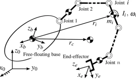
We will introduce the RNS formalism with a simple example: a free-floating serial-link chain in zero gravity. This model will be used to derive the basic notations. The most relevant application would be a free-floating space robot comprising a rigid-link manipulator arm mounted on a rigid-body satellite – the floating base of the system (see Fig. 1).
The manipulator joints are assumed actuated while the base is not. First, we will derive the RNS formalism at ve-locity level, based on the momentum conservation condition. Then, the full dynamics will be taken into consideration.
3.1 Momentum-based derivation
End-effector
Joint Joint 2
Joint 1
x
0y
0z
0x
by
bz
bJoint
Figure 1.Model of a free-floating base serial-link chain.
(Featherstone, 2008), wherein the angular momentum part is written w.r.t. the CoM of the CRB:
Lc≡ "
p lc
#
=McVc. (2)
Subscript (◦)c denotes quantities defined w.r.t. coordinate
frame{c}fixed at the CRB CoM, which is an inertial (non-accelerating) frame in the absence of external forces, and thus under momentum conservation. The linear part of mo-mentum is p=Pn
j=0mj˙rj=mt˙rc while the angular part is
lc=Pnj=0
Ijωj+mjrj×˙rj
, where mj, Ij, rj,ωj, stand for
link j mass, inertia matrix, CoM position and angular veloc-ity, respectively, the latter three given in inertial coordinates. mtdenotes the total mass of the CRB system, rcandVcstand
for its CoM position and spatial velocity, respectively. Ma-trix Mc(q) is a 6×6 block-diagonal matrix having Mv≡mtU
andcMω≡Pn
j=0
Ij+mjjr×ccr×j
as upper and lower blocks, respectively, where U is the 3×3 unit matrix1. Henceforth,
constants will be denoted by an over-bar. Since the above momentum is a conserved quantity, we then denote it as ¯Lc.
With the above notations, the momentum conservation equation has the simplest possible form McVc=L¯c.
Nev-ertheless, it is desirable to employ inertial properties familiar from fixed-base manipulator descriptions. For this purpose, it is necessary to redefine spatial momentum w.r.t. the base frame{b}:
Lb=
"
p
br
c×p+lc #
, (3)
The motion of the robot can then be represented at the veloc-ity level as:
MbVb+Mbmθ˙=Lb, (4)
whereVbdenotes the spatial velocity of the base. Matrix Mb(q)=
"
Mv Mvω
MTvω Mω #
∈ <6×6
1Note thatjr
c×=(cr×j) T=−cr×
j.
is the inertia matrix of the system regarded as an CRB, matrix
Mbm(q)= h
MTvm MTωm iT
∈ <6×n
is a block submatrix of the system inertia matrix, called henceforthcoupling inertia matrix. The block submatrices in the above terms are:
Mvω≡ −mtbr×c (5)
Mvm≡mtbJc (6)
Mω≡bI0+
n
X
j=1 b
Ij+mjjr×b br×
j
(7)
Mωm≡
n
X
j=1 b
IjbJωj+mjbr×j
bJ
v j
(8)
where it was assumed that link 0 is the base. Jc,Jv jdenote
the CRB CoM and link- j CoM velocity Jacobians, respec-tively, while Jωj is the link- j angular velocity Jacobian. As
can be inferred from the leading superscript, all these quan-tities are defined w.r.t. the base frame{b}(see also Masutani et al., 1989). We should note that the coupling inertia subma-trix Mvm, contributing to translational motion of the CRB, is
identical to the system CoM Jacobian, up to a multiplicative constant (the total mass). For a free-floating system, trans-lational motion is considered less important than rotational. But for the other MBS discussed below, e.g. flexible-base and humanoid robots, the case is just the opposite. We should also note that usually, it is assumed that initial spatial momentum is null.
The momentum component MbVb, appearing on the l.h.s.
of Eq. (4), can be interpreted twofold. First, assuming a nonzero initial momentum and immobilized manipulator joints, the component has the meaning of conserved CRB momentum. This is a trivial case. Usually, and henceforth, zero initial momentum will be assumed, such that the condi-tion ¯Lc=0=Lb holds. Then, the above component has the
meaning of CRB momentum occurring in reaction to the ma-nipulator motion (s.t. MbVb=−Mbmθ, ˙˙ θ,0). Therefore, we
will henceforth refer to MbVb asreaction momentum. The
other momentum component Mbmθ, on the other hand, has˙
the meaning of momentumimposedupon the CRB (i.e. in-cluding the base) via manipulator motion. We will refer to it as thecoupling momentum(Nenchev et al., 1996) and denote it as:
Lbm≡Mbmθ.˙ (9)
Equation (4) can be solved for the manipulator joint ve-locities, needed as input variables for velocity-based system motion control. Since the equation is linear in the velocities, its solution type depends upon the number of manipulator joints n. In the case of a six-DOF manipulator (n=6), for example, the unique solution is:
˙
More interesting is the case of a kinematically redundant ma-nipulator (n>6). We have then an underdetermined system, with the general solution (Nenchev, 1989):
˙
θ=−M#bmMbVb+Pbmθ˙a, (11)
where (◦)# denotes a generalized inverse, P
(◦) stands for
a null-space projector and ˙θa is an arbitrary vector
dimen-sioned as joint velocity.
Apparently, the coupling inertia matrix comprises a non-trivial kernel. The infinite set of joint velocities from the kernel can be derived via the second term on the r.h.s.{θ˙rl:
Pbmθ˙a,∀θ˙a}. This is the set ofreactionless joint velocities;
these velocities do not impose any momenta on the base, and thus, manipulator motion will becompletely dynamically de-coupledfrom the motion of the base. Note also that the re-actionless joint velocities constitute the set of solutions of homogeneous equation
Mbmθ˙=0, (12)
which stands for coupling momentum conservation. Hence, we can conclude that reactionless motion (and hence, com-plete dynamical decoupling) can be achieved if and only if the coupling momentum is conserved (Nenchev et al., 1996). Further on, note that the set{θ˙rl}has the structure of a
man-ifold in joint space, e.g. similarly to the selfmotion manman-ifold known from studies on kinematically redundant manipula-tors (Burdick, 1989). We will call it the reactionless mo-tion manifold. The manifold depends upon the rank of the RNS projector: rankPbm=n−6. With a seven-DOF
articu-lated manipulator, for example, the manifold will be just one-dimensional. Hence, reactionless motions can be derived via the differential equation:
˙
θ=bnbm, (13)
where b is an arbitrary scalar with dimension of angular speed. nbm(q)∈ker Mbm will be called reactionless vector
field. The integral curves, projected onto workspace via the direct kinematics, will be referred to asreactionless paths.
In general, it is desirable to have a larger set of reaction-less paths. One possibility to achieve this is increasing the number of manipulator joints. Another possibility is to rede-fine the coupling inertia matrix (and thus its kernel) w.r.t. a suitable subset of base coordinates. For a free-floating space robot, most important is the orientation of the satellite base. Hence, we may redefine the above equations to ignore base translation variables. Then, the rank of the null-space projec-tor will increase to n−3. Because of its fundamental role, the kernel has been named as theReaction Null Space(Nenchev et al., 1999).
Let us focus now on the other joint velocity component in Eq. (11), i.e. reaction momentum mapped via a gener-alized inverse of the coupling inertia matrix. Recall first that velocity-based redundancy resolution schemes, similar
to that in Eq. (11), are known from studies of kinematically redundant manipulators (Konstantinov et al., 1981) – the so-called “task-of-priority” type schemes (Nakamura et al., 1987). Such schemes give the possibility to address dual-task control scenarios: typically end-link motion control via the generalized-inverse component, plus an additional con-trol task (e.g. optimization of a suitable measure, obstacle avoidance etc), via the null-space component. Note also that quite often the Moore-Penrose generalized inverse (the pseu-doinverse) is used in such schemes, since it yields a locally optimal solution for the joint-velocity norm (Nenchev, 1989). Also, in this case, the two components of the general so-lution (11) become orthogonal, yielding joint-space decom-position into two orthogonal complementary subspaces. In our case, when the pseudoinverse is used in Eq. (11), the re-spective joint velocity component yields optimal inertial cou-pling in terms of minimizing that part of the total kinetic en-ergy, that is due to the dynamical coupling between the base and the rest of the links. We will refer to this energy as the
coupling kinetic energy:VT
bMbmθ. Such energy minimiza-˙
tion is a highly desirable feature. The reason is that typical motion control scenarios are dual-task ones: e.g. reaction-less motion control via the null space component (a feedfor-ward control component), plus error compensation control for small base attitude errors, via the pseudoinverse compo-nent (a feedback control compocompo-nent)2. Coupling energy op-timization will thereby yield better performance with regard to error dynamics.
In conclusion, via the null space and the pseudoinverse, we obtain adecomposition formalism that can be quite useful for motion analysis, planning and control of various unfixed-base systems, as will be shown henceforth with a few more examples. This decomposition is the essence of the RNS method.
3.2 Dynamics-based derivation
To account for the presence of external forces, we consider the full dynamics of the free-floating robot:
Mb Mbm
MTbm Mm ˙ Vb ¨ θ + Cb cm = Fb τ +
bTT
e JT
Fe, (14)
where quantities, not yet introduced, are:
Mm ∈ <n×n: manipulator inertia matrix
J ∈ <6×n: manipulator Jacobian matrix
cm ∈ <n : manipulator nonlinear force
Cb ∈ <6 : CRB nonlinear force
τ ∈ <n : joint torque vector
Fb ∈ <6 : external force at the base
Fe ∈ <6 : external force at the end-link
2See e.g. the discussion on possible motion control tasks in
Hereby, we assumed that external forces may act upon the base (Fb) and/or the end-link (Fe). In fact, the base forceFb term could be assigned a broader role to include base con-straint and/or actuator forces. This will allow us, in what follows, to model other types of systems with the same equation, e.g. a free-flying space robot with attitude con-trolled base (i.e. using reaction/momentum wheels as actua-tors) and/or flexible appendages, a flexible-base manipulator, a humanoid robot, and others.
Let us focus now on the upper part of the equation of mo-tion. It can be rewritten as:
MbV˙b+Mbmθ¨+Cb=Fext, (15)
whereFext=Fb+bTTeFe denotes the external forces. This
equation represents the dynamics of the CRB since only ex-ternal forces are present. The dynamic equilibrium can then be expressed asFd−Fext=0, whereFdis thedynamical force
obtained as time derivative of CRB momentum:
Fd≡
d
dtLb=Mb ˙
Vb+Mbmθ¨+M˙bVb+M˙bmθ.˙ (16)
The last two terms on the r.h.s. denote the CRB nonlinear forceCb≡M˙bVb+M˙bmθ. The two manipulator motion com-˙
ponents, on the other hand, represent the spatial force:
Fbm≡
d
dtLbm=Mbm ¨
θ+M˙bmθ.˙ (17)
We will refer toFbm as theimposed force, in the sense that
the force is imposed upon the CRB via manipulator motion. It should be apparent then that any motion along a reaction-less path (i.e. reactionreaction-less motion), conserves coupling mo-mentum (cf. Eq. 12), and implies hence a null imposed force Fbm=0.
From (15), it is straightforward to derive manipulator joint acceleration, needed in dynamical control schemes, e.g. re-solved acceleration control (Luh et al., 1980) or computed torque control (Craig, 2004). We will skip the trivial nonre-dundant case and focus on the more interesting kinematically redundant manipulator case:
¨
θ=M+bm(Fext−MbV˙b− Cb)+Pbmθ¨a, (18)
where ¨θa denotes an arbitrary n-vector with dimension of
joint acceleration. With the help of this vector, reactionless manipulator motion can be generated in a feedforward man-ner, since the respective joint acceleration component Pbmθ¨a
yields coupling momentum conservation. In addition, the pseudoinverse acceleration component will be useful in dual-task scenarios, e.g. for feedback compensation of small atti-tude errors, as already explained. Thereby, full dynamic de-coupling between the two subtasks will be ensured, as al-ready discussed in the last subsection.
In computed torque controllers, the joint torque is used as control input. It can be derived by inserting the above joint
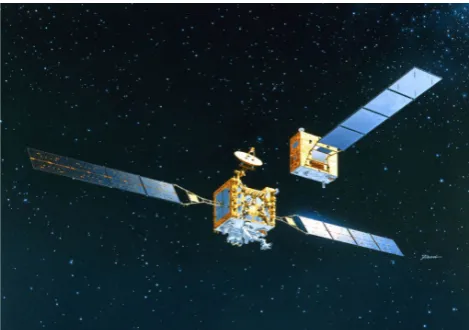
Figure 2.Artistic rendering of the ETS-VII space robot mission. A six-DOF manipulator arm is mounted on the larger satellite thus constituting a free-floating space robot with serial arm structure. (Courtesy of JAXA – the Japan Aerospace Exploration Agency, Oda, 2000).
acceleration into the lower part of Eq. (14):
τ=MTbmV˙b+Mmθ¨−JTFe+cm (19)
=
MTbm−MmM+bmMb ˙
Vb
+
MmM+bm bTT
e−J
T
Fe
+cm+MmM+bm(Fb− Cb)+MmPbmθ¨a.
3.3 Implementation issues
The RNS method has been experimentally verified via both simulations and on-orbit experiments with the ETS-VII space robot system (see Fig. 2). The goal was to confirm the usefulness of reactionless manipulator motion on-orbit. Since the space robot was freely floating in micro-gravity environment, the presence of external forces (e.g. solar pres-sure, air drag, gravity gradient) has been ignored during the relatively short time interval of the experiment (about 20 min). It was possible then to employ the momentum con-servation condition to obtain a suitable velocity-based reac-tionless motion generator, via the null-space solution (13) in a feedforward manner. The trajectories were generated in ad-vance off-line and then transferred to the robot arm on-orbit for execution. The experimental results can be found e.g. in (Yoshida et al., 2000).
4 Application to flexible-base and macro/mini manipulator systems
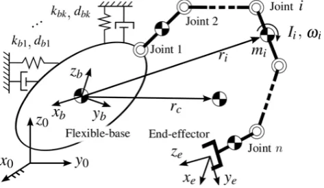
Figure 3.An example of a flexible-base robot: Rollin’ Justin – a robot with a humanoid upper body mounted on a wheeled mo-bile base with flexible suspension (Courtesy of DLR – the German Aerospace Center, Borst et al., 2009).
access to a dangerous site. Another example is a robot com-prising a humanoid upper body mounted on a mobile base via flexible suspension, e.g. the robot Rollin’ Justin designed at DLR (Borst et al., 2009) (see Fig. 3). There are also so-called macro/mini manipulator systems, consisting of a dexterous manipulator (the mini part) attached to the end-link of a large manipulator (the macro part). The latter ensures positioning capability of the mini part within a large workspace. Due to its structure, the large arm usually has inherent flexibilities in the links and/or joints. Hence, the end-link of the large arm can be thought of as a flexible base for the mini part, whereby, the flexible base can be characterized as a compos-ite rigid body. Two such systems exist on the International Space Station: the large Canadarm 2 with the Special Pur-pose Dexterous Manipulator “Dextre” (Coleshill et al., 2009) and the large Japanese Experiment Module Remote Manip-ulator System (JEMRMS) with the Small Fine Arm (SFA) (see Fig. 4) (Sato and Wakabayashi, 2001).
Such flexible-base robots require a special motion gener-ation technique and respective control in order to minimize the reactions at the flexible base. Otherwise, essential
high-Figure 4.An example of a macro/mini manipulator system: model of the Japanese Experiment Module (JEM) “Kibo” on the Inter-national Space Station with the large Remote Manipulator System (JEMRMS) and the Small Fine Arm (SFA) attached.
precision positioning and/or path tracking capabilities of the dexterous manipulator(s) may degrade significantly. The Re-action Null Space method with its joint-space decomposition formalism can be employed in a straightforward manner to ensure reactionless motion, via the RNS component, in com-bination with inertial damping control of flexible-base vibra-tions, via the pseudoinverse component.
4.1 Single-body flexible base
The simplest possible case is a serial rigid-link manipulator attached to a single-body flexible base (see Fig. 5). First, we will assume that the spatial elastic forces, constraining the motion of the flexible base, are expressed via the following Fbappearing in Eq. (14):
Fb=−DbVb−Kb∆Xb. (20)
Db,Kb∈ <6×6denote base spatial viscous damping and stiff
-ness, respectively, and∆Xbstands for base spatial
displace-ment from the equilibrium. With this notation, the CRB dy-namics (Eq. 15) become:
MbV˙b+DbVb+Kb∆Xb=−Mbmθ¨−M˙bmθ˙ (21)
=−Fbm
where we assume that no external force acts at the end-link and that the nonlinear term ˙MbVb is ignorable. From this
relation, it becomes apparent that by designing a suitable im-posed forceFbm, additional damping can be injected into the
system, e.g.:
Fbmref=GbVb, (22)
Gbdenoting the additional spatial damping gain. In the case
of a redundant manipulator, the control input is the joint ac-celeration:
¨
Figure 5.Model of a single-body flexible base manipulator system.
This equation has the same structure as Eq. (18). Hence, a dual-task control scenario can be achieved wherein the two subtasks will be completely dynamically decoupled: the RNS component Pbmθ¨a ensures reactionless motion, while
the pseudoinverse component is useful for inertial damping control of any existing vibrations, whereby the coupling en-ergy will be minimized. In addition, the equation is suitable for both velocity control and torque control. In the former case, velocities are obtain via integration; in the latter case, the joint torques are obtained in a similar way as Eq. (19), i.e. by substitution of the joint acceleration into the lower part of the equation of motion.
Further on, it is easy to confirm that the closed-loop dy-namics are:
MbV˙b+(Db+Gb)Vb+Kb∆Xb=0, (24)
i.e. they appear in the form of unforced dynamics of a spa-tial mass-damper-spring system. Then, proper damping can be achieved with a suitably chosen damping gain Gb (Hara
et al., 2010).
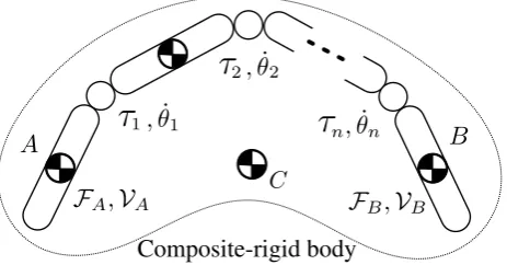
4.2 Composite rigid-body flexible base (macro/mini system)
The macro part of a macro/mini manipulator system can be thought of as an composite rigid-body flexible base, under the assumption that the joints and/or links have inherent flexibilities. Having in mind the JEMRMS/SFA system, we will further assume that both macro and mini system parts comprise a serial-link structure. The generalized coordinates
will be denoted as q=hqTM qTm iT
, qM∈ <k and qm∈ <n
standing for the joint variables of the macro and mini part, respectively. The structure of the equation of motion resem-bles that of a single-body base, whereby subscript (◦)M
re-places the base subscript (◦)bto denote quantities associated
with the macro part:
"
MM MMm
MTMm Mm # "
¨qM
¨qm #
+
"
cM
cm #
=
"
−DM˙qM−KM∆qM
τ
#
. (25)
Note that, usually, it is assumed that the macro part joints are passive (Morimoto et al., 2001). Hence, their joint torque does not appear in the equation. Joint damping and stiffness, however are present; they are expressed via diagonal matri-ces DM,KM∈ <k×k, respectively. Other quantities associated
with the macro part include joint space inertia MM∈ <k×k
and nonlinear force cM∈ <k.
From the upper part of the equation, the macro/mini dy-namics are expressed as:
MM¨qM+DM˙qM+KM∆qM=τM, (26)
whereτM≡ −MMm¨qm−cMplays the role of a torque imposed
upon the joints of the macro part via the motion of the mini part. We focus again on inertia coupling, represented via ma-trix MMm∈ <k×n. If we assume that the mini part has more
joints than the macro3, then the kernel of this matrix is non-trivial. Reactionless motion, and hence, complete dynamical macro/mini decoupling, can then be achieved via joint accel-erations derived from the kernel – the Reaction Null Space of the macro/mini system. Using the RNS joint space decompo-sition property and following the derivations introduced with the previous example, we can devise a control law for the mini part, in resemblance to Eq. (23), to ensure a dual-task control scenario involving reactionless motion in combina-tion with inertial damping of the macro vibracombina-tion:
¨qm=−M+Mm(GM˙qM+M˙Mm˙qm)+PMm¨qma, (27)
where GM∈ <k×k is a diagonal gain matrix for additional
damping injection. The second term on the r.h.s. represents the reactionless joint acceleration component, PMmdenoting
the RNS projector and ¨qma standing for an arbitrary vector
dimensioned as mini-part joint acceleration.
4.3 Humanoid upper body on flexible base
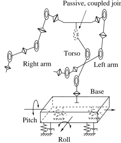
This example is interesting because the system has a tree-like structure comprising two arms of seven DOFs each, at-tached to the upper end of a torso of three DOF. The other end of the torso is attached to the flexible base that is rep-resented as a single body with two elastic DOFs (pitch and roll), see Fig. 7. There is an abundant 15 degree of redun-dancy w.r.t. reactionless motion. From a practical viewpoint, additional constraints are to be imposed. A simple example, as discussed in (Wimbock et al., 2009), is specific motion task assignment for one of the arms, let’s say the right arm, while using the other arm, or the other arm and the torso, to compensate for the disturbance imposed on the base. For these two scenarios, the degree of redundancy reduces to five or eight, respectively. The equation of motion can be written
3In the JEMRMS/SFA model we used (Hara et al., 2010) k=
3 and n=9 (in Fig. 4, the respective joint sets are{q1,q2,q3}and
End-effector
Joint Joint 2 Joint 1
Joint
Figure 6.Model of an composite rigid-body flexible base system (a macro/mini manipulator).
as:
Mb Mbr Mbc
MTbr Mr Mrc
MTbc MTrc Mc ˙ Vb ¨qr ¨qc + Cb cr cc + Gb gr gc =
−DbVb−Kb∆Xb
τr τc , (28)
where newly appearing subscripts (◦)r and (◦)c stand for
“right arm” and “compensating subsystem” (i.e. left arm or left arm plus torso), respectively. The “g”-terms denote grav-ity forces. The CRB dynamics are selected from the upper part:
MbV˙b+DbVb+Kb∆Xb=−Mbr¨qr−Mbc¨qc− N, (29)
whereN collects all nonlinear and gravity terms. Under the assumption that the right arm acceleration ¨qr is known from the task assignment, the control acceleration for the compen-sating subsystem can be selected as:
¨qc=M+bc(Gc˙qc−Mbr¨qr− N)+Pbc¨qca, (30)
where ¨qca is an arbitrary vector dimensioned as compensat-ing subsystem joint acceleration. The form of this equation is the same as in the previous examples, Eqs. (23) and (27). Additional damping can be injected via gain Gc, and also,
re-actionless motion can be achieved via the RNS term Pbc¨qca.
Experimental data can be found in Wimbock et al. (2009).
5 Application as an Operational Space Method
So far, we have confirmed that via the RNS decomposition, complete dynamical decoupling between the unfixed base and the rest of the links can be achieved. An interesting ques-tion is whether the same approach can be applied to the ma-nipulator’s end-effector e.g. of a serial-link chain, instead to the base. The answer is trivial; the implication is an alter-native to the Operational Space formulation (OSF) (Khatib,
Pitch
Roll
Right arm
Base
Torso
Left arm
Passive, coupled joint
Figure 7.Model of Rollin’ Justin – humanoid upper body on flexi-ble base (Wimbock et al., 2009).
1987). This sections gives the details of the derivation and a qualitative comparison between the two formulations.
5.1 Brief overview of the Operational Space formulation The importance of the OSF, e.g. in motion/force control scenarios for fixed-base manipulators, is quite well known. More recently, the formulation is being also applied to more sophisticated MBS like humanoid robots (Sentis and Khatib, 2010). A brief overview is included here for completeness. The underlying equation is:
Me(θ) ˙V+Ce(θ,θ)˙ +Ge(θ)=F, (31)
whereVdenotes end-link spatial velocity,
Me(θ)=
(J(θ)M−1 m(θ)J
T(θ)−1
∈ <6×6, (32)
is theoperational space inertia (Khatib, 1987), Mm(θ) and
J(θ) standing for the manipulator inertia matrix and the ma-nipulator Jacobian, respectively. Ce, Ge and F denote the
Coriolis and centrifugal force, the gravity force and the force imposed on the end-link, respectively. These forces are ex-pressed in end-link coordinates and are obtained from the manipulator joint-space dynamics via the transpose of the inertia-weighted generalized inverse4of the Jacobian:
J#M(θ)=M−m1(θ)J
T(θ)M
e(θ)
4Referred to also as the “dynamically consistent” inverse
Composite-rigid body
Figure 8.Model of a unfixed-base serial-link chain. The system constitutes a single composite rigid body, C denoting its CoM.
as the underlying transform. It should be apparent that the end-link dynamics formulation (31) will fail when the ma-nipulator Jacobian becomes rank-deficient, i.e. at akinematic singularity.
5.2 RNS-based end-link dynamics formulation
We will use the free-floating dynamics notation from Sect. 3.2. To avoid confusion, we rename the two end-links of the free-floating chain as A and B (see Fig. 8). Without loss of generality, we will pick up end-link A as the link of reference. The equation of motion is then:
MA MAm
MTAm Mm ˙ VA ¨ θ + CA cm + GA gm = FA τ +
ATT
B JT
Fb, (33)
gravity terms inclusively. The upper part is the CRB dynam-ics; the coordinates are those of end-link A but the inertial properties are those of the entire system. The lower part, on the other hand, contains generalized force components of a fixed-base manipulator, link A being the “fixed base”. The manipulator is composed of all bodies except link A; because end-link A coordinates are used, quantities Mm, cmand J are
those of the fixed-base manipulator, link B being its end-link. Henceforth we switch the roles of the two end-links: link A becomes the “real” end-link, while link B is the (unfixed) base. The latter will be later on constrained to obtain a fixed-base system. In this way, results comparable to the fixed-fixed-base OSF dynamics can be obtained. With this preparation, it is apparent that the CRB dynamics
MAV˙A+CA+GA=FA+ATTBFB−MAmθ¨ (34)
represent system dynamics in terms of end-link coordinates, i.e. similar to Eq. (31) in OSF. Several remarks are due. First, note that in the above equation, end-link acceleration ˙VA
and forceFAare explicitly present. Therefore, there was no
need to invoke a transformation from joint-space dynamics, i.e. via the inertia-weighted generalized inverse, as it was the
case with the OSF. Second, differently from the OSF end-link dynamics (Eq. 31), the above equation can be applied even at kinematic singularities. Third, the inverse dynamics prob-lem for the joint accelerations can be solved directly from the above dynamical relation in end-link coordinates. This is due to the term−MAmθ¨ appearing on the r.h.s. of the
equa-tion. This term stands for inertial coupling between the end-link and the rest of the end-links; it makes joint motion explicitly visible as an end-link dynamical force. The respective joint torque can then be derived from the lower part of Eq. (33).
These properties of the RNS end-link dynamics can be considered as advantageous, e.g. when compared to the OSF end-link dynamics. There are also other differences: under the RNS formulation, end-link forceFAis a “real” external
force; it is not merely a mapping of the joint torque vector as in the OSF. Similarly, nonlinear forceCAand gravity force GA are “true” CRB forces, and not merely mappings of the respective joint-space terms. Also, the presence of forceFB may be of some advantage, e.g. in situations when reaction force control will be needed (such as in the case of a hu-manoid robot).
5.3 Inverse dynamics and controller design
The inverse dynamics problem plays an important role in model-based control design, i.e. in computed-torque control methods. The OSF provides the possibility to design con-trollers that ensure complete dynamical decoupling of the end-effector. A motion/force controller, proposed in (Khatib, 1987), calculates the end-link reference force as:
Fref=Fmref+Fκref, (35)
Fmref=Me(θ)S ˙Vref+Ce(θ,θ)˙ +Ge(θ)+Me(θ) ˙SV,
Fκref=S⊥Fcref,
whereFmrefandFκrefare two components referring to end-link motion and contact force, respectively. S is a selection matrix suitably defined to specify the unconstrained (motion) direc-tions, while S⊥is its complement, specifying the constrained directions from the reference contact forceFc. In the case of a redundant manipulator, the respective computed-torque controller can be written as:
τ=JTFref+U−JTJ#TMτrefa , (36) whereτrefa denotes an arbitrary vector dimensioned as joint
torque. Torque component JTFrefis the nominal joint torque
θ
1θ
2θ
3m
1m
2m
3a
1l
1a
2l
2a
3l
3x
0z
0A
B
k
Bzd
Bzfixed base
x
cz
cθ
*r
θ
3θ
1m
3m
2m
1a
3l
3a
2l
2a
1l
1x
cz
cA
B
k
Azd
Azx
0z
0r
fixed base
θ
2: passive joint
: active joint
(a) (b)
Figure 9.Equivalent planar five-link four-joint manipulator models used in: (a) RNS and (b) Operational Space formulations. In (a), the “root” link is end-link A (the end-effector); In (b), the “root” link is end-link A (the base). The passive joint at the end-link appears since the end-link orientation is ignored.
Below we will show how similar dynamically-consistent relations can be derived under the RNS formulation. The joint acceleration can be obtained from Eq. (34) as:
¨
θ=M#AmFA−MAV˙A+ATTBFb− CA− GA
+PAmθ¨a, (37)
where (◦)#denotes a generalized inverse of the coupling in-ertia matrix. The second term on the r.h.s. is a vector from the kernel of this matrix, ¨θadenoting an arbitrary vector with
di-mension of joint acceleration. Hence, there is an infinite set of joint accelerations {θ¨rl: ¨θrl=PAmθ¨a,∀θ¨a}that would not
disturb the state of the end-link. Any acceleration from the above set can therefore be characterized asreactionless joint accelerationw.r.t. the state of the end link. This implies com-plete dynamical decoupling of the end link from the rest of the links. Henceforth, we refer to the kernel as theReaction Null Space w.r.t. the end-link.
It follows that there is also an infinite set of joint torque vectors{τrl=Mmθ¨rl,∀θ¨a}that do not affect the imposed
end-link force and hence, maintain the state of the end-end-link. The joint torque is obtained by inserting joint acceleration (37) into the lower part of (33):
τ=τn+τrl, (38)
where
τn=
MTAm−MmM#AmMA
˙
VA (39)
+MmM#AmFA+
MmM#Am ATT
B−J
T
Fb
+cm+gm−MmM#Am(CA+GA)
is the nominal component of the solution. It includes end-link A’s acceleration and force that can be used as refer-ence inputs in a motion/force controller similar to Eq. (36).
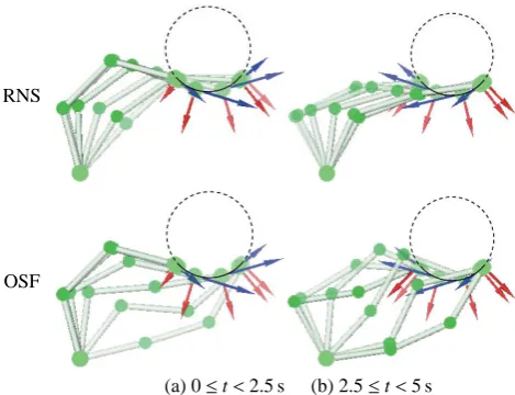
RNS
OSF
(a) 0≤t<2.5 s (b) 2.5≤t<5 s
Figure 10.Snapshots from the simulation with two equivalent pla-nar 3R redundant manipulators tracking a semi-circular path and ap-plying a desired force. The blue/red arrows denote the desired mo-tion/force vectors, respectively. No null-space motion is involved. In the RNS simulation (upper graphs) no significant arm reconfig-uration is observed; in the OSF simulation (lower graphs), on the other hand, significant arm reconfiguration (spurious link motion) is observed (Hara et al., 2012).
Since the other joint-toque component τrl is reactionless
w.r.t. the end-effector, it should be apparent that we obtained a dynamically-consistent relationship in the sense of Khatib. Note, however, that in our formulation the nominal com-ponentτn represents a dynamical torque; it doesnot stem
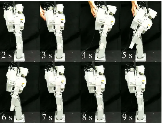
Figure 11.Snapshots from the experiment with a HOAP-2 robot responding to an unknown continuous-force disturbance on the back (sagittal plane). The so-called Hip strategy has been realized under velocity-based reactionless motion with a three-link two-joint model in the sagittal plane (Nenchev and Nishio, 2008; Kanamiya et al., 2010).
property will not be lost. Actually, τn constitutes an
in-finite number of dynamically-consistent relationships be-cause there is an infinite set of generalized inverses for MAm, namely{M#Am: MAmM#AmMAm}. Each specific
gener-alized inverse will provide a specific dynamically-consistent scheme. Such schemes would be usually constructed to sup-port task-dependent redundancy resolution, quite in a similar fashion as known from past studies on kinematically redun-dant manipulators (Nenchev, 1989).
As an example, let us pick up the Moore-Penrose gener-alized inverse (pseudoinverse). Local optimality can then be achieved, the minimized quantity being that part of total ki-netic energy that is due to the dynamical coupling between end-link A and the rest of the links:VATMAmθ. Note that un-˙
der the Operational Space formulation, the minimized quan-tity is the total kinetic energy (Khatib, 1987): 1
2V
TM
eV.As
apparent from Eq. (32), this is a highly nonlinear function due to the inverse of a quadratic form of the Jacobian ma-trix. This means that in the (not necessarily small) vicinity of kinematic singularities, excessive fluctuation in the joint velocity can be expected. In contrast, the coupling kinetic energy, minimized under the RNS formulation, is quite well behaved, even within a relatively small vicinity of ill-defined inertial coupling, i.e. where the coupling inertia matrix be-comes rank deficient. We can summarize then: with the RNS formulation we can expect better performance in terms of joint motion than with the OSF, and equal performance in terms of end-link motion/force control. This has been exam-ined experimentally, with two simple models (see Fig. 9)
per-forming the same motion/force control task, realized with the respective nominal component (no null-space motion) (Hara et al., 2012). The significant difference in terms of joint-space motion can be confirmed from the animation snapshots in Fig. 10. With the RNS motion/force control formulation, link motion does not deviate much from the initial configuration. This indicates the lack of large peaks in joint velocity. With the OSF, on the other hand, spurious link motion is observ-able, which is due to the highly nonlinear dynamic transform (the inertia-weighted generalized inverse) used in the formu-lation and the resulting peak joint velocities in the vicinity of kinematic singularities.
6 Application to humanoid robots
A humanoid is an underactuated system and its balance con-trol can be achieved only via the imposed/reaction forces, when the feet are in contact with the ground. The prevailing research approach is to make use of the Zero Moment Point5 (Vukobratovi´c and Borovac, 2004) that can provide informa-tion about roll/pitch momenta on the feet. These momenta are sufficient for balance control on flat ground, when frictional forces are ignored. A more interesting situation, however, is balancing/walking on uneven ground, and also, when con-sidering the presence of friction and other unknown distur-bances. To deal with such problems, full spatial force control
5In the static case, the ZMP is the projection of the total CoM
108 D. N. Nenchev: Reaction Null Space of a multibody system with applications in robotics
disturbance on the back (sagittal plane). The so-called Hip strategy has been realized under velocity-based
re-actionless motion with a three-link two-joint model in the sagittal plane (Nenchev and Nishio, 2008), (Kanamiya
et al., 2010).
Fig. 12.
Snapshots from the experiment with a HOAP-2 robot responding to an unknown continuous-force
disturbance on the shoulder (frontal plane). (a)-(c), (i) and (j): Ankle strategy; (d)-(g): Lift-leg strategy; (h):
Transition between the two strategies. Two different models in the frontal plane are used; Ankle strategy:
three-link two-joint model; Lift-leg strategy: four-link three-joint model (Yoshida et al., 2011).
21
Figure 12.Snapshots from the experiment with a HOAP-2 robot responding to an unknown continuous-force disturbance on the shoulder (frontal plane). (a–c, i and j) ankle strategy; (d–g) lift-leg strategy; (h) transition between the two strategies. Two different models in the frontal plane are used; Ankle strategy: three-link two-joint model; Lift-leg strategy: four-link three-joint model (Yoshida et al., 2011).
at the feet via the imposed/reaction force relation is neces-sary. This can be achieved with the RNS formulation in a straightforward manner, as should be apparent from the ap-plications discussed so far.
6.1 Planar humanoid models and balance strategies The RNS method has been applied to the balance problem in terms of both joint velocity, i.e. using momentum balance (Nenchev and Nishio, 2008; Kanamiya et al., 2010; Yoshida et al., 2011), and joint torque (Tamegaya et al., 2008). In the former case, balance strategies in response to an unknown ex-ternal disturbance (continuous or impact type) have been de-vised, based on the analysis of human behavior under similar circumstances. For example, when the disturbance is applied on the back while standing upright, the so-called hip strat-egy may be invoked (Shumway-Cook and Horak, 1989), i.e. bending in the hips and motion in the ankles in the opposite direction. This strategy can be readily realized with a sim-ple three-link (foot, leg, upper body), two-joint (ankle, hip) planar model in the sagittal plane. The unfixed-base motion dynamics are then represented as:
Mf Mfm
MTfm Mm ˙ Vf ¨ θ + Cf cm + Gf gm = Ff τ +
fTT
e
JTe
Fe, (40)
where subscripts “f” and “e” stand for “foot” and “external”, respectively. With this notation, the foot is considered the un-fixed base,Ffdenoting the force at the foot resulting from the specific ground contact conditions and including three com-ponents: vertical ground reaction force, horizontal frictional force and foot moment, the latter being the most important for balance.
First, we consider the following simplifying assumptions: the foot is always in contact with the ground (the acceler-ation of the CoM vertically upward is restricted) and also,
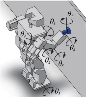
1 2 3 4 5 6 7
Figure 13.A small humanoid robot cleaning a vertical surface: spa-tial seven-DOF model, with active (θ1 throughθ5) and passive (θ6
andθ7) joint coordinates.
the horizontal frictional force is sufficiently large. The ditions are then similar to those when using ZMP-based con-trol. We can then ignore the two force components at the foot and rewrite the dynamics to include just the foot moment. Then, the coupling inertia matrix Mfm∈ <1×2will comprise
a nontrivial kernel. The related null-space projector will be denoted as Pfm. Further on, if we assume as initial conditions
static equilibrium and null foot moment, i.e.Vf,V˙f andFf
all zero, then this state (and thus balance) can be maintained with reactionless motion. In terms of joint accelerations, re-actionless motions are derived from the CRB dynamics (i.e. the upper part of the equation of motion):
¨
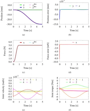
Figure 14.Simulation results under RNS-based dynamical motion/force feedback control: the desired motion trajectory in hand coordinates is a 30 mm straight line downwards (along -z); the hand force (x component) is regulated thereby to 5 Nm.
This is the reactionless joint acceleration set that was used to generate a compliant response to the disturbance by bend-ing in the hips, followed up by standbend-ing upright configuration recovery, after the disturbance disappeared (see Fig. 11). Fur-ther on, since reactionless motion implies coupling momen-tum conservation, as explained in Sect. 3.1, reactionless mo-tion generamo-tion in terms of joint velocity is also possible. This property was used to realize the Hip strategy under velocity (and thus position) control.
The same approach was adopted with regard to distur-bances at the shoulder, within the frontal plane (Yoshida et al., 2011). Snapshots from respective experiments are shown in Fig. 12. Initially, again, a three-link model was used to ensure compliant upper-body response, with paral-lel motion of the legs (considered as a single-link motion – the Ankle strategy: (a)–(c), (i) and (j)). When the disturbance persisted, the robot responded by shifting the CoM further
over the right foot and lifting the left leg (Lift-leg strategy: (d)–(g)). Thereby, the model was extended by one more link and a joint.
6.2 Spatial humanoid models and motion/force control As mentioned in Sect. 5, the RNS formalism suits espe-cially operational-space type motion/force control task sce-narios with humanoid robots. As an example, consider a spa-tial humanoid model with seven DOFs: six for the arm and one for the ankle joint (see Fig. 13a). The robot’s task is to clean a vertical surface. Three hand coordinates are in-volved to complete the task: two tangential coordinates (y and z) for trajectory tracking within the vertical plane, and one normal coordinate (x) for force tracking (Sato et al., 2011). Note that the wrist comprises a passive U-joint; its joint coordinates (θ6andθ7) are available via the loop-closure
equation. The remaining five joint coordinates (θ1 through
θ5) are actively controlled. Thus, the system has two
redun-dant DOFs. The equations from Sect. 5 can be applied in a straightforward manner, whereby end-links A and B denote the robot hand and the foot, respectively. Below we present simulation data, wherein the joint acceleration is computed via Eq. (37). Thereby, the pseudoinverse is used as a gen-eralized inverse, the feet are assumed stationary and fixed (i.e. the six-dimensional spatial forceFB is determined via
the Lagrange multiplier method). No use of the null space acceleration is made (¨θa=0). Thus, feedback control only
is applied to track the desired y-z hand (unfixed-base) mo-tion trajectory (a 30 mm straight line downwards), regulating thereby the desired force to 5 Nm. The graphs are shown in Fig. 14. It is seen that the motion/force control task could be performed in a stable manner, and without excessive joint velocity and torque. The null-space component, though not used currently, is available e.g. for balance control (roll/pitch control) of the feet. This will be confirmed with upcoming experiments.
7 Conclusions
This study summarizes results based on the application of the Reaction Null Space approach. The RNS, defined as the ker-nel of the coupling inertia – a submatrix of the system inertia matrix – provides a joint space decomposition formalism that can be quite useful for motion analysis, motion generation and motion control of various unfixed-base systems, such as free-floating space robots, flexible-base and macro/mini robot systems, as well as humanoid robots. Via the null space and the pseudoinverse mapping of the coupling inertia, the joint space can be decomposed into two complementary or-thogonal subspaces. Thus, two oror-thogonal joint space com-ponents in terms of joint velocity, joint acceleration and joint torque can be derived, with the properties of complete dy-namical decoupling and locally optimal dydy-namical coupling, respectively. The former component induces a reactionless vector field and the respective reactionless-motion manifold in joint space. The latter component, on the other hand, im-poses a spatial-force constraint via manipulator motion, that can be used for locally optimized control of the unfixed base,
e.g. base orientation, base vibration suppression or foot re-action control of a free-floating space robot, a flexible-base robot and a humanoid robot, respectively.
Acknowledgements. The contribution of Naoyuki Hara and Ryohei Okawa with figures and HOAP-2 model simulation data is acknowledged.
Edited by: A. M¨uller
Reviewed by: I. Sharf and one anonymous referee
References
Abiko, S. and Yoshida, K.: Adaptive Reaction Control for Space Robotic Applications with Dynamic Model Uncertainty, Adv. Robotics, 24, 1099–1126, doi:10.1163/016918610X501264, 2010.
Book, W. and Lee, S. H.: Vibration Control of a Large Flexible Ma-nipulator by a Small Robotic Arm, in: American Control Confer-ence, 1377–1380, 1989.
Borst, C., Wimbock, T., Schmidt, F., Fuchs, M., Brunner, B., Zacharias, F., Giordano, P. R., Konietschke, R., Sepp, W., Fuchs, S., Rink, C., Albu-Schaffer, A., and Hirzinger, G.: Rollin’ Justin – Mobile platform with variable base, in: 2009 IEEE Inter-national Conference on Robotics and Automation, 1597–1598, doi:10.1109/ROBOT.2009.5152586, 2009.
Briot, S., Arakelian, V., and Le Baron, J.-P.: Shaking force minimization of high-speed robots via centre of mass acceleration control, Mech. Mach. Theory, 57, 1–12, doi:10.1016/j.mechmachtheory.2012.06.006, 2012.
Burdick, J.: On the inverse kinematics of redundant manipulators: characterization of the self-motion manifolds, in: 1989 IEEE In-ternational Conference on Robotics and Automation, 264–270, doi:10.1109/ROBOT.1989.99999, 1989.
Cheng, D.: End-point Control of a Flexible Structure Mounted Ma-nipulator Based on Wavelet Basis Function Networks, in: 2005 IEEE/RSJ International Conference on Intelligent Robots and Systems, Workshop on Robot Vision for Space Applications, 29– 34, 2005.
Cocuzza, S., Pretto, I., and Debei, S.: Reaction torque control of redundant space robotic systems for orbital maintenance and simulated microgravity tests, Acta Astronaut., 67, 285–295, doi:10.1016/j.actaastro.2009.05.007, 2010.
Coleshill, E., Oshinowo, L., Rembala, R., Bina, B., Rey, D., and Sindelar, S.: Dextre: Improving maintenance operations on the International Space Station, Acta Astronaut., 64, 869–874, doi:10.1016/j.actaastro.2008.11.011, 2009.
Cong, P. C. and Sun, Z. W.: Preimpact Configuration Anal-ysis of Dual-Arm Space Manipulator Capturing Object, J. Aerospace Eng., 23, 117–123, doi:10.1061/ (ASCE)AS.1943-5525.0000016, 2010.
Craig, J.: Introduction To Robotics: Mechanics & Control, 3rd Edn., Prentice Hall, 2004.
Elfizy, A., Bone, G., and Elbestawi, M.: Design and control of a dual-stage feed drive, Int. J. Mach. Tool. Manu., 45, 153–165, doi:10.1016/j.ijmachtools.2004.07.008, 2005.
Fattah, A. and Agrawal, S. K.: Design and simulation of a class of spatial reactionless manipulators, Robotica, 23, 75–81, doi:10.1017/S0263574704000670, 2005.
Featherstone, R.: Rigid Body Dynamics Algorithms, Springer US, Boston, MA, doi:10.1007/978-0-387-74315-8, 2008.
Featherstone, R. and Khatib, O.: Load Independence of the Dynam-ically Consistent Inverse of the Jacobian Matrix, Int. J. Robot. Res., 16, 168–170, doi:10.1177/027836499701600203, 1997. Finat, J. and Gonzalez-Sprinberg, G.: A semianalytic approach to
the modelling and control of the biped gait for the design of in-teractive orthoses in rehabilitation tasks, in: 11th IEEE Interna-tional Workshop on Robot and Human Interactive Communica-tion, 350–355, doi:10.1109/ROMAN.2002.1045647, 2002. Gorce, P.: Dynamic postural control method for biped in
un-known environment, IEEE T. Syst. Man Cyb. A, 29, 616–626, doi:10.1109/3468.798065, 1999.
Gouo, A., Nenchev, D., Yoshida, K., and Uchiyama, M.: Motion control of dual-arm long-reach manipulators, Adv. Robotics, 13, 617–631, doi:10.1163/156855399X01846, 1998.
Hanson, M. L. and Tolson, R. H.: Reducing flexible base vibrations through local redundancy resolution, J. Robotic Syst., 12, 767– 779, doi:10.1002/rob.4620121106, 1995.
Hara, N., Kanamiya, Y., and Sato, D.: Stable path tracking with JEMRMS through vibration suppression algorithmic singulari-ties using momentum conservation, in: 10th International Sym-posium on Artificial Intelligence, Robotics and Automation in Space, 214–221, 2010.
Hara, N., Handa, Y., and Nenchev, D.: End-link dynamics of re-dundant robotic limbs: The Reaction Null Space approach, in: 2012 IEEE International Conference on Robotics and Automa-tion, 299–304, doi:10.1109/ICRA.2012.6224627, 2012. Hyon, S.-H., Osu, R., and Otaka, Y.: Integration of multi-level
postural balancing on humanoid robots, in: 2009 IEEE Inter-national Conference on Robotics and Automation, 1549–1556, doi:10.1109/ROBOT.2009.5152434, 2009.
Kaigom, E. G., Jung, T. J., and Rossmann, J.: Optimal Mo-tion Planning of a Space Robot with Base Disturbance Minimization, in: 11th Symposium on Advanced Space Technologies in Robotics and Automation 2011 (As-tra2011), 1–6, http://www.mmi.rwth-aachen.de/?public100, http://robotics.estec.esa.int/ASTRA/Astra2011/Papers/04B/ FCXNL-11A06-2139450-1-2139450GuiffoKaigom.pdf, 2011. Kanamiya, Y., Ota, S., and Sato, D.: Ankle and hip balance
control strategies with transitions, in: 2010 IEEE Interna-tional Conference on Robotics and Automation, 3446–3451, doi:10.1109/ROBOT.2010.5509785, 2010.
Khatib, O.: A unified approach for motion and force con-trol of robot manipulators: The operational space formula-tion, IEEE Journal on Robotics and Automaformula-tion, 3, 43–53, doi:10.1109/JRA.1987.1087068, 1987.
Khatib, O.: Inertial Properties in Robotic Manipulation: An Object-Level Framework, Int. J. Robot. Res., 14, 19–36, doi:10.1177/027836499501400103, 1995.
Konno, A., Myojin, T., Matsumoto, T., Tsujita, T., and Uchiyama, M.: An impact dynamics model and sequential optimization to generate impact motions for a humanoid robot, Int. J. Robot.
Res., 30, 1596–1608, doi:10.1177/0278364911405870, 2011. Konstantinov, M. S., Markov, M. D., and Nenchev, D. N.:
Kine-matic Control of Redundant Manipulators, in: 11th International Symposium on Industrial Robots, 561–568, Tokyo, 1981. Lampariello, R., Heindl, J., Koeppe, R., and Hirzinger, G.:
Reactionless Control for two Manipulators Mounted on a Cable-Suspended Platform, in: 2006 IEEE/RSJ Interna-tional Conference on Intelligent Robots and Systems, 91–97, doi:10.1109/IROS.2006.281777, 2006.
Lee, S. H. and Book, W.: Robot Vibration Control Using Iner-tial Damping Forces, in: VIII CISM-IFToMM Symposium on the Theory and Practice of Robots and Manipulators (Ro. Man. Sy. ’90), 252–259, Cracow, Poland, http://hdl.handle.net/1853/ 39161, 1990.
Lew, J., Trudnowski, D., Evans, M., and Bennett, D.: Mi-cro manipulator motion control to suppress maMi-cro ma-nipulator structural vibrations, in: 1995 IEEE International Conference on Robotics and Automation, 3, 3116–3120, doi:10.1109/ROBOT.1995.525728, 1995.
Luh, J., Walker, M., and Paul, R.: Resolved-acceleration control of mechanical manipulators, IEEE T. Automat. Contr., 25, 468– 474, doi:10.1109/TAC.1980.1102367, 1980.
Masutani, Y., Miyazaki, F., and Arimoto, S.: Modeling and sensory feedback control for space manipulators, in: NASA Conf. Space Telerobotics, 1989.
Morimoto, H., Kasama, Y., Doi, S., and Wakabayashi, Y.: Mo-tion Control of the Small Fine Arm for the Japanese Experi-ment of the International Space Station, in: Int. Conf. Advanced Robotics, 187–195, 2001.
Murray, R. M., Li, Z., and Sastry, S. S.: A Mathematical Introduc-tion to Robotic ManipulaIntroduc-tion, CRC Press, 1994.
Nakamura, Y., Hanafusa, H., and Yoshikawa, T.: Task-Priority Based Redundancy Control of Robot Manipulators, Int. J. Robot. Res., 6, 3–15, doi:10.1177/027836498700600201, 1987. Nenchev, D., Yoshida, K., and Umetani, Y.: Introduction of
redundant arms for manipulation in space, in: IEEE In-ternational Workshop on Intelligent Robots, 88, 679–684, doi:10.1109/IROS.1988.593682, 1988.
Nenchev, D., Umetani, Y., and Yoshida, K.: Analysis of a redundant free-flying spacecraft/manipulator system, IEEE T. Robotic. Au-tom., 8, 1–6, doi:10.1109/70.127234, 1992.
Nenchev, D., Yoshida, K., and Uchiyama, M.: Reaction null-space based control of flexible structure mounted manipulator systems, in: Proceedings of 35th IEEE Conference on Decision and Con-trol, 4, 4118–4123, doi:10.1109/CDC.1996.577417, 1996. Nenchev, D., Yoshida, K., Vichitkulsawat, P., and Uchiyama, M.:
Reaction null-space control of flexible structure mounted ma-nipulator systems, IEEE T. Robotic. Autom., 15, 1011–1023, doi:10.1109/70.817666, 1999.
Nenchev, D. N.: Redundancy resolution through local op-timization: A review, J. Robotic Syst., 6, 769–798, doi:10.1002/rob.4620060607, 1989.
Nenchev, D. N. and Nishio, A.: Ankle and hip strategies for balance recovery of a biped subjected to an impact, Robotica, 26, 643– 653, doi:10.1017/S0263574708004268, 2008.
Oda, M.: Experiences and lessons learned from the ETS-VII robot satellite, in: 2000 IEEE International Conference on Robotics and Automation. (Cat. No. 00CH37065), 1, 914–919, doi:10.1109/ROBOT.2000.844165, 2000.
Osumi, H. and Saitoh, M.: Control of a Redundant Manipulator Mounted on a Base Plate Suspended by Six Wires, in: 2006 IEEE/RSJ International Conference on Intelligent Robots and Systems, 73–78, doi:10.1109/IROS.2006.281669, 2006. Ott, C., Albu-Schaffer, A., and Hirzinger, G.: A Cartesian
Compliance Controller for a Manipulator Mounted on a Flexible Structure, in: 2006 IEEE/RSJ International Con-ference on Intelligent Robots and Systems, 4502–4508, doi:10.1109/IROS.2006.282539, 2006.
Papadopoulos, E. and Dubowsky, S.: Coordinated manipula-tor/spacecraft motion control for space robotic systems, in: Proceedings. 1991 IEEE International Conference on Robotics and Automation, April, 1696–1701, IEEE Comput. Soc. Press, doi:10.1109/ROBOT.1991.131864, 1991.
Parsa, K., Angeles, J., and Misra, A. K.: Control of Macro-Micro Manipulators Revisited, J. Dyn. Syst.-T. ASME, 127, 688, doi:10.1115/1.1870039, 2005.
Piersigilli, P., Sharf, I., and Misra, A.: Reactionless capture of a satellite by a two degree-of-freedom manipulator, Acta Astro-naut., 66, 183–192, doi:10.1016/j.actaastro.2009.05.015, 2010. Sato, F., Nishii, T., Takahashi, J., Yoshida, Y., Mitsuhashi,
M., and Nenchev, D.: Experimental evaluation of a trajec-tory/force tracking controller for a humanoid robot clean-ing a vertical surface, in: 2011 IEEE/RSJ International Conference on Intelligent Robots and Systems, 3179–3184, doi:10.1109/IROS.2011.6094615, 2011.
Sato, N. and Wakabayashi, Y.: JEMRMS design features and top-ics from testing, in: 6th International Symposium on Artificial Intelligence and Robotics & Automation in Space, 1–7, 2001. Sentis, L. and Khatib, O.: Compliant Control of
Mul-ticontact and Center-of-Mass Behaviors in Humanoid Robots, IEEE Transactions on Robotics, 26, 483–501, doi:10.1109/TRO.2010.2043757, 2010.
Sharf, I.: Active Damping of a Large Flexible Manipulator With a Short-Reach Robot, J. Dyn. Syst.-T. ASME, 118, 704, doi:10.1115/1.2802346, 1996.
Shui, H., Wang, J., and Ma, H.: Optimal Motion Planning for Free-Floating Space Robots Based on Null Space Approach, 2009 In-ternational Conference on Measuring Technology and Mecha-tronics Automation, 845–848, doi:10.1109/ICMTMA.2009.556, 2009.
Shumway-Cook, A. and Horak, F. B.: Vestibular Rehabilitation: an exercise approach to managing symptoms of vestibular dysfunc-tion, Seminars in Hearing, 10, 196–209, 1989.
Stephens, B.: Humanoid push recovery, in: Humanoids 2007 – 7th IEEE-RAS International Conference on Humanoid Robots, 589– 595, doi:10.1109/ICHR.2007.4813931, 2007.
Tamegaya, K., Kanamiya, Y., Nagao, M., and Sato, D.: Inertia-coupling based balance control of a humanoid robot on unstable ground, in: Humanoids 2008 – 8th IEEE-RAS International Conference on Humanoid Robots, 151–156, doi:10.1109/ICHR.2008.4755960, 2008.
Torres, M. and Dubowsky, S.: Minimizing spacecraft attitude distur-bances in space manipulator systems, J. Guid. Control Dynam., 15, 1010–1017, doi:10.2514/3.20936, 1992.
Torres, M., Dubowsky, S., and Pisoni, A.: Vibration con-trol of deployment structures’ long-reach space manipula-tors: The P-PED method, in: Proceedings of IEEE Interna-tional Conference on Robotics and Automation, 3, 2498–2504, doi:10.1109/ROBOT.1996.506538, 1996.
Vukobratovi´c, M. and Borovac, B.: Zero-Moment Point – Thirty Five Years of Its Life, Int. J. Hum. Robot., 01, 157–173, doi:10.1142/S0219843604000083, 2004.
Wimbock, T., Nenchev, D., Albu-Schaffer, A., and Hirzinger, G.: Experimental study on dynamic reactionless motions with DLR’s humanoid robot Justin, in: 2009 IEEE/RSJ International Conference on Intelligent Robots and Systems, 5481–5486, doi:10.1109/IROS.2009.5354528, 2009.
Xu, W., Liu, Y., Liang, B., Xu, Y., and Qiang, W.: Autonomous Path Planning and Experiment Study of Free-floating Space Robot for Target Capturing, Journal of Intelligent and Robotic Systems, 51, 303–331, doi:10.1007/s10846-007-9192-3, 2007.
Yoshida, K., Nenchev, D., Vichitkulsawat, P., Kobayashi, H., and Uchiyama, M.: Experiments on the point-to-point operations of a flexible structure mounted manipulator system, Adv. Robotics, 11, 397–411, doi:10.1163/156855397X00399, 1996.
Yoshida, K., Hashizume, K., Nenchev, D., Inaba, N., and Oda, M.: Control of a space manipulator for autonomous target capture -ETS-VII flight experiments and analysis-, in: AIAA Guidance, Navigation and Control Conference and Exhibit, 1297–1306, 2000.
Yoshida, Y., Takeuchi, K., Sato, D., and Nenchev, D.: Pos-tural balance strategies for humanoid robots in response to disturbances in the frontal plane, in: 2011 IEEE Interna-tional Conference on Robotics and Biomimetics, 1825–1830, doi:10.1109/ROBIO.2011.6181555, 2011.