Parallel simulations of 3d DC borehole resistivity measurements with
goal-oriented self-adaptive hp finite element method
M.Paszyński1*, D.Pardo2, V.Calo3
1
AGH University of Science and Technology, Krakow, Poland [email protected]
2
The University of the Basque Country, Bilbao, Spain and IKERBASQUE (Basque Foundation of Science) [email protected]
2
King Abdullah University of Science and Technology, Thuwal, Saudia Arabia [email protected]
*Corresponding author
Abstract
In this paper we present a parallel algorithm of the goal-oriented self-adaptive hp Finite Element Method (hp-FEM) with shared data structures and with parallel multi-frontal direct solver. The algorithm generates in a fully automatic mode (without any user interaction) a sequence of meshes delivering exponential convergence of the prescribed quantity of interest with respect to the mesh size (number of degrees of freedom). The sequence of meshes is generated from the prescribed initial mesh, by performing h (breaking elements into smaller elements), p (adjusting polynomial orders of approximation) or hp (both) refinements on selected finite elements. The new parallel implementation utilizes a computational mesh shared between multiple processors. We describe the parallel self-adaptive hp-FEM algorithm with shared computational domain, as well as its efficiency measurements. The presentation is enriched by numerical simulation of the problem of through casing 3D DC borehole resistivity measurement simulations in presence of invasion.
Keywords: hp Finite Element Method, goal-oriented adaptivity, shared data structure
1. Introduction
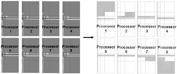
Fig. 1. The shared domain decomposition where the copy of computational mesh is duplicated on every processors, but degrees of freedom are stored in distributed manner. The data structure
takes no more than 10% of the total memory utilized during the solver call
In this paper we propose an alternative parallelization technique, based on the shared domain decomposition paradigm, illustrated on the right panel in Fig. 1. The entire data structure with the computational mesh is stored on every processor. However, the computations performed over the mesh are shared between processors. It is done by assigning the so-called processor owners to particular mesh elements, and executing computations over these elements by assigned processors. This is usually performed by sharing the algorithm‘s loops by many
processors, followed by mpi_allreduce call merging results.
The paper is an extended version of the presentation for the International Conference on Computational Science ICCS 2012 [Calo et. al. 2011]. The structure of the paper is the following. In Section 2 entitled Automatic hp Adaptivitywe introduce an overview of the self-adaptive goal-oriented algorithm. In the following Section 3 entitled Data Structure supporting
mesh refinements we introduce details of the classes necessary to implement the hp adaptive
algorithm. Section 4 entitled Parallel fully automatic goal-oriented hp Finite Element Method deals with the parallelization of the self-adaptive goal-oriented algorithm. Finally, Sections 5 and 6 entitled Computational problem formulation and Numerical results present the simulation results and the scalability of the parallel algorithm.
2. Automatic hp adaptivity
A general sequential algorithm for the fully automatic hp adaptation can be described is the following steps.
(2) The computational problem is solved over the coarse mesh and the approximate solution uhp is obtained.
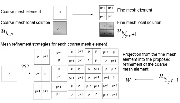
(3) The coarse mesh is globally hp-refined in order to produce the fine mesh. It is done by breaking each finite element into four son elements and increasing the polynomial order of approximation by one. This will be the reference mesh used for calculation of the interpolation error over the coarse mesh.
(4) The computational problem is solved on the fine mesh and the approximate solution
1 , 2p
h
u is obtained.
(5) As the relative error estimator for the coarse mesh, the difference (in H1-seminorm) between the coarse and the fine mesh solutions is taken. The optimal refinements are selected based on the calculated error estimators for the subset of the coarse mesh elements with higher relative error estimators. Selected elements are either broken into smaller son elements (this is so called h-refinement) isotropically (4 sons) or anisotropically (2 sons in the same direction) or the polynomial order of approximation is increased on element edges or interiors (this is so called p-refinement), or both. This is illustrated in Fig. 2.
The optimal refinements are selected independently over each coarse mesh element. It is done in a way to provide maximal error decrease rate given by:
nrdof w u u u rate p h p h p h 1 1 , 2 1 , 1 , 2 max (1)
where nrdof is the number of added degrees of freedom during the considered refinement, w is the solution for proposed refinement strategy, obtained by utilizing the projection based
interpolation (Demkowicz 2004) from the fine mesh solution , 1
2p
h
u into the considered
refined element, uh ,p 1 uh,p
2
is the relative error estimation over the current coarse mesh
with respect the fine mesh and uh ,p1w 2
is the relative error estimation for the refinement
strategy proposed for the coarse mesh element with respect to the fine mesh. Thus, we seek for a refinementproviding the best error decrease rate with a minimum increase in the number of degrees of freedom.
(1) The selected refinements are executed over the coarse mesh to obtain the new optimal
mesh.
Fig. 2. Many possible refinements of a coarse mesh element
The selection of the optimal refinements for the coarse mesh finite elements is actually performed in two steps, in order to limit the number of possibilities considered in point 6). First, the optimal refinements are selected for finite element edges, and then the optimal refinements for element interiors are selected, with restriction to known optimal refinements for element edges. The relative error measurements over element edges are performed in the H½ seminorm.
The above energy-norm based adaptive algorithm has been further generalized to the case of goal-oriented adaptivity. The necessary modifications included solving the so-called ―dual‖ problem over the same coarse and fine grids, and estimate goal-oriented errors as a combination of the solutions of both direct and dual problems. From the parallel data structures point-of-view, these modifications implied duplicating the number of degrees-of-freedom in order to accommodate solution of the dual problem.
3. Data Structure supporting mesh refinements
In this section we introduce data structure supporting mesh h and p refinements performed by the self-adaptive hp finite element method algorithm.
In the following part of the section, the element, node and vertex classes are introduced
Class:
Element
Attributes:
character(5) : type - 'quadr‘, 'trian' the information about type of the element (currently, the code supports only quadrilateral elements)
integer(4) : neighbors – pointers to 4 adjacent elements stored in ELEMS table
integer(4) : vertices – pointers to 4 vertices stored in VERTS table
integer(5) : nodes - pointers to 4 edge nodes and 1 middle node
stored in NODES table
integer(4) : bcond - boundary conditions for 4 element edges
integer : processor_owner - processor owning the element
Class:
Vertex
Attributes:
double(2) : geom_coord – geometrical coordinates of the node
integer : father – pointer to father node in NODES table
integer : father_iel - pointer to father initial mesh element
in ELEMS table (if any)
double : solution d.o.f. - degree of freedom (coefficient of local shape functions) utilized for local approximation of the solution
integer(4) : processor_owners - list of processors owning the vertex
integer :: nr_processor_owners – size of the list
Class:
Node
Attributes:
character(4) : type - type of the node: 'medg' for edge node,
'mdlq' for middle node
integer : order - order of approximation
integer : father – pointer to father node in NODES table
integer : ref_kind – flag coding refinement type of the node
integer, dimension(:) : vertex_sons - dynamically allocated table storing pointers to all son vertices for broken edge or interior nodes
integer, dimension(:) : edge_sons - dynamically allocated table storing pointers to all edge son nodes for broken edge or interior nodes
integer, dimension(:) : interior_sons - dynamically allocated table storing pointers to all interior son nodes for broken interior nodes
double, dimension(:,:) : geometry_d.o.f. - geometrical degrees of freedom utilized to express geometry of curvilinear edges, expressed as a combination of node shape functions
double, dimension(:,:) : solution_d.o.f. - degrees of freedom
(coefficients of local shape functions) utilized for local approximation of the solution
integer : kref - required refinement for the node, used during the virtual refinements
integer(4) : processor_owners - list of processors owning the vertex
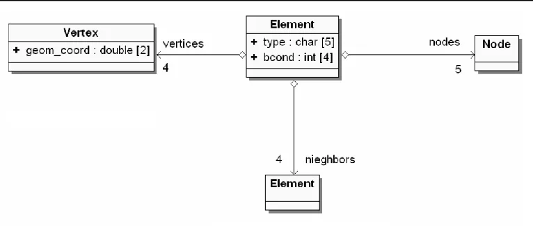
Fig. 3. Relations between Element, Node and Vertex
The classes are stored in the following ELEMS, VERTS and NODES collections
Collections of objects:
type(Element), pointer, dimension(:) :: ELEMS
dynamically allocated table of Element class objects
type(Node), pointer, dimension(:) :: NODES
dynamically allocated table of Node class objects
type(Vertex), pointer , dimension(:) :: VERTS
dynamically allocated table of Vertex class objects
The Element class objects are created for initial mesh elements only. Each initial mesh element may have up to four adjacent initial mesh elements. The pointers to neighbors (actually indices of neighbors in ELEMS collection) are stored in bcond array. Let us discuss relations between Element, Node and Vertex classes presented in Figure 3.
Each element consists of four vertices, four edges and one interior. Element vertices
correspond to Vertex class objects. Each Element class object aggregates the vertices
list of four Vertex objects. Each Element class object aggregates the nodes list of four
Node objects of ‘medg’ type and one Node object of ‘mdle’ type. Four Node class objects are related to element edges, and these objects have attribue type=’medg’. One
Node class object is related to element interior, and this Node class object has attribue
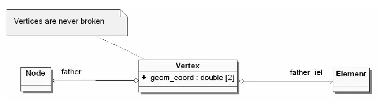
Fig. 4. Links stored by Vertex class object
When an element edge is broken, one new graph vertex representing element vertex and two new graph vertices representing element edges are created. These newly created graph vertices are again represented by one Vertex class object and two Node class objects, with type=‘medg‘. The Node class object with type=‘medg‘, representing element edge, aggregates a list of vertex_sons and edge_sons. When the edge is broken, the ref_kind attribute of the Node class object is set to 1, and references to newly created Vertex class and Node class objects are stored on these lists. This is illustrated in Figure 5.
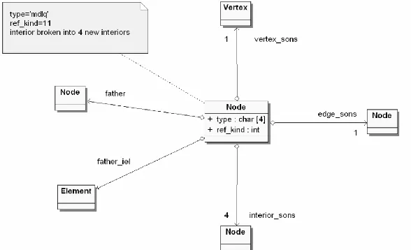
When an element interior is broken in both, horizontal and vertical directions, one new graph vertex representing element vertex, four new graph vertices representing element edges, and four new graph vertices representing element interiors are created. These newly created graph vertices are again represented by one Vertex class object, four Node class objects, with type=‘medg‘ and four Node class objects, with type=‘mdle‘. The Node class object with type=‘mdle‘, representing element interior, aggregates a list of vertex_sons, edge_sons and interior_sons. When the interior is broken in both directions, the ref_kind attribute of the Node class object is set to 11, and references to newly created Vertex class and Node class objects are stored on these lists. This is illustrated in Figure 6.
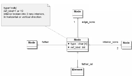
The application supports also anisotropic mesh refinements, thus, element interior can be broken in one direction. When an element interior is broken in one direction, one new graph vertex representing element edge, and two new graph vertices representing element interiors are created. These newly created graph vertices are again represented by one Node class objects,
with type=’medg’ and two Node class objects, with type=’mdle’. The Node class
object with type=’mdle’, representing element interior, aggregates a list of
Fig. 5. Relations between Element, Node and Vertex class objects for broken element edge
4. Parallel fully-automatic goal-oriented hp Finite Element Method
In this section, we present the parallel version of the fully automatic goal-oriented hp adaptivity, implemented under the shared domain decomposition paradigm. The new parallel algorithm can be summarized in the following steps:
Fig. 7. Relations between Element, Node and Vertex class objects for element interior broken in one direction
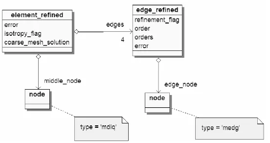
(1) The coarse initial mesh is generated on every processor. The initial mesh elements are assigned to different processors, by filling processor_owner attribute of the element object. It is performed either by interfacing with the ZOLTAN library (ZOLTAN), or by utilizing simple row-wise mesh partitioners for two dimensional meshes. The element‘s processor_owner attribute is filled on every processor, in other words, each processor knows processor owners of all elements. The element edges and vertices are assigned to processor owners. It is performed by browsing all elements and filling processor_owners lists located at element node or vertex objects. This is illustrated in Figure 8. The element_refined objects are created for each active finite element. This is illustrated in Figure 9. The middle_node links are related with interior nodes of active finite elements, represented by node objects with type=‘mdlq‘. The edge_refined objects are created for all active finite element edges. The edge_node links are related with element edge nodes, represented by node objects with type=‘medg‘. Notice, that element_refined objects (related to active finite elements) do not correspond to element objects (related to the initial mesh elements only).
(2) The computational problem is solved over the current coarse mesh, by utilizing multi-frontal parallel direct solver [Paszyński et al. 2010; Paszyński and Schaefer 2010]. Each processor stores the local solution vector at its active finite element node and
vertex objects, in the solution_d.o.f. attribute, see Figure 8. The coarse
mesh solution d.o.f. are also recorded at coarse_mesh_solution arrays of
elements_refined objects.
Fig. 9. Additional data structure managing mesh refinements over the distributed data structure
(1) The global hp refinement is executed over the coarse mesh in order to construct the reference fine mesh. This is performed by every processor over the entire data structure. Each finite element from the coarse mesh is partitioned into four new finite elements, and the polynomial order of approximation is uniformly raised by one. This is done by executing isotropic h refinement over each element interior node object,
as well as refinement over each element edge node object. Also, the
order_of_approximation attribute is increased for each active node (for each leaf node object).
(2) The processor_owners of newly created node and vertex objects are filled based on the information inherited from father node objects.
(3) The computational problem is solved again over the fine mesh by utilizing the multi-frontal parallel direct solver [Paszyński et al. 2010; Paszyński and Schaefer 2010]. Each processor stores the local solution vector at its active finite element node and
vertex objects, in the solution_d.o.f. attribute. Notice that the coarse mesh solution is still stored at parent nodes as well as at elements_refined objects. For the case of goal-oriented adaptivity, we also solve for the ―dual‖ problem.
(4) Each processor loops through its active elements and computes the relative error estimation over the element
1 1
1 , 2 1 , 2
H p h H p h hp
u u
u
(2)
with uhp being the coarse mesh solution restored from the element_refined objects, and
1 , 2p
h
u being the fine mesh solution restored from the solution_d.o.f. attribute of active
finite element node and vertex objects. The relative error is stored in the error attribute of the element_refined objects. For the case of goal-oriented adaptivity, the relative error estimation over the element also incorporates terms corresponding to the solution of the dual problem.
(1) The maximum element relative error is computed, and elements with the relative error
(2) For elements with strong gradient of the error in one direction, the isotropy_flag
attribute of the element_refined object is set to enforce the element refinement in one direction.
(3) Different refinement strategies are considered for element edges, by utilizing the formula
K K p h K p h K p h p h K p h p h nrdof w u w u u u u u , 2 1 1 , 2 , 2 1 1 , 2 , 2 1 , 1 , 2 , 2 1 , 1 , 2 ~ ~ ~ ~ (3)with K denoting an element, uhp the coarse mesh solution restored from the
element_refined objects, , 1 2p
h
u the fine mesh solution restored from active finite
element node and vertex objects, and w being the projection based interpolant of the fine
mesh solution , 1
2p
h
u into the considered edge refinement. Tilde symbol denotes solution of
the ―dual‖ problem needed for goal-oriented adaptivity. The H½
seminorm is utilized to measure
the relative error over an element edge. The selected refinement is stored in edge_refined
object. If an element edge is going to be p refined, the ref_flag attribute for the edge is set to 1, and the proposed order of approximation is stored at order attribute. If an element edge is going to be h refined, the ref_flag attribute for the edge is set to -1, and the proposed orders of approximation for son edges are stored at orders attribute array. These estimations are performed by every processor over active finite elements assigned to the processor. Thus, the optimal refinement information is stored in distributed manner in element_refined
and edge_refined objects. These estimations are performed only for edges of elements with relative error estimation larger than 33% of the maximum relative error.
(1) The proposed refinement data (ref_flag, order and orders attributes of
edge_refined object as well as isotropy_flag of element_refined object) are broadcasted to all processors.
(2) The fine mesh is deallocated and the coarse mesh is restored.
(3) The selected optimal refinements are executed for element edges. This is done by all processors over the entire data structure. It can be done, since we broadcasted the proposed refinement data. Some edges are h refined: one new vertex object and two new edge node objects are created are connected to the original edge node. The order of approximation for new node objects is taken from orders attribute array of edge_refined object. Some edges are p refined, and the new order of
approximation is taken from order attribute of edge_refined object. Some edge
refinements are modified based on the isotropy_flag from
element_refined objects.
(4) Different element interior node refinements are considered for elements. This is done by utilizing the formula
relative estimated error above 33% of the maximum relative error.
(1) The proposed interiors refinement data (refinement_flag and orders
attributes of element_refined objects) are broadcasted to all processors.
(2) The selected optimal refinements are executed for element interiors. This is done by all processors over the entire data structure. Some elements are h refined: new edge and interior node objects and vertex objects (for isotropic h refinement) are created and connected to the original interior node. The order of approximation for new node
objects is taken from orders attribute array of element_refined object. Some
elements are p refined, and the new orders of approximation are taken from orders
attribute of element_refined object.
(3) The minimum rule is enforced over the entire data structure: the order of approximation over element edges is set to be equal to the minimum of orders for adjacent element interiors. This is done by all processors over the entire data structure. Thus, an identical copy of the new optimal mesh is stored on every processor.
(4) The element_refined and edge_refined objects are deallocated.
If the maximum error is still greater than the required accuracy of the solution, the new optimal mesh becomes a coarse mesh and the next iteration is executed.
5. Computational problem formulation
In this section we present exemplary parallel simulations for the 3D DC resistivity logging measurement simulation problem. The problem consists in solving the conductive media equation
impJ
u
(5)
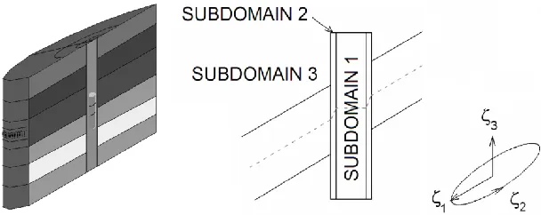
in the 3D domain with different formation layers presented in Fig. 10. There is a logging tool with one transmitter and two receiver electrodes in the borehole. The tool is shifted along the borehole. The reflected waves are recorded by the receiver electrodes in order to determine location of the oil formation in the ground. Of particular interest to the oil industry are 3D simulations with deviated wells, where the angle between the borehole and formation layers is
sharp (
0
90
). This 3D problem can be decomposed as a sequence of coupled 2D problemset al. 2010], the variational formulation in the new system of coordinates consists in finding
1 D DH
u
u
such that:
1 2 2 ˆ , ˆ , D L L H v f v v u (6)where new electrical conductivity of the media
ˆ
:
J
1
J
1TJ
andf
ˆ
:
f
J
withimp
J
f
being the gradient of the impressed current, and
1 2 3
3 2 1 , , , ,
x x x
J
(7)
stands for the Jacobian matrix of the change of variables from the Cartesian reference to non-orthogonal systems of coordinates, and
J
det
J
is its determinant. We take Fourier seriesexpansions in the azimuthal
2 direction
, ,
,
2;3 1 3 2 1
l l jl l e uu
(8)
, ,
,
2;3 1 3 2 1
m m jm m e (9)
, ,
,
2;3 1 3 2 1
l l jl l e ff
(10)
where
2 0 2 2 2
1 ue d
ul jl ,
2 0 2 2 2
1
d e jm
m and
2 0 2 2 2 1 d e f
fl jl and j is the imaginary
unit. We introduce symbol Fl such that applied to a scalar function u it produces the l
th
Fourier modal coefficient ul, and when applied to a vector or matrix, it produces a vector or matrix of
the components being lth Fourier modal coefficients of the original vector or matrix components.
Using the Fourier series expansions we obtain the following variational formulation:
Find Fl
u Fl
uD HD1
such that:
1 2 2 2 2 22 , ˆ
ˆ , D L jl l L m l j m
l e vF f e v H
v F u F D D (11)
The Einstein‘s summation convention is applied with respect to l,m. We select a
mono-modal test function jk2
ke v
v . Thanks to the orthogonality of the Fourier modes in L2,
extension of [Pardo et al. 2008] and they include also the case in presence of 10 cm and 50 cm invasion. The problem geometry can be described by using cylindrical coordinates
,,z
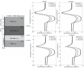
.Fig. 10. Left panel: The borehole, the tool with receiver and transmitter electrodes and the deviated formation layers. Right panel: The non-orthogonal system of coordinates
(1) Four (one current and three voltage) 2 × 5-cm ring electrodes located 8 cm from the
axis of symmetry and moving along the vertical direction (z axis). Voltage (collector) electrodes are located 100, 125, and 150 cm above the current (emitter) electrode, respectively.
(2) Borehole: a cylinder A of radius 10 cm surrounding the axis of symmetry
, , : 10cm
A x z with resistivity R0.1m.
(3) Casing: a pipe (cylindrical shell) B of thickness 1.27 cm surrounding the axis of
symmetry B
x,,z
:10cm11.27cm
, with resistivity R105m.(4) Formation material 1: a subdomain C defined by
, , : 11.27cm,0cm 100cm
C x z z with resistivity R m
4
10 .
(5) Formation material 2: a subdomain D defined by
, , : 11.27cm,50cm 0cm
(6) Formation material 3: a subdomain E defined by
, , : 11.27cmor 100cm
E x z z with resistivity R5m.
Notice that each point on the plot requires a solution of the 3D problem, and the point corresponds to the value of the solution at receiver electrode, computed with a very high accuracy thanks to the goal-oriented hp adaptive methodology. The logging tool has been shifted along the borehole, from the relative position of 2meters down to -2meters, and we perform a new simulation for each position of the logging tool. We refer to [Pardo et al. 2008] for more details. Figure 12 presents the scalability tests of the parallel solver algorithm. The parallel version of the solver has been tested on the two dimensional mesh with 576 finite elements with uniform polynomial order of approximation p=2 and 10 Fourier modes utilized to approximate the solution in its third direction (thus, total number of d.o.f. per node is equal to 20). We refer to [Paszyński et al. 2010; Paszyński and Schaefer 2010; Paszyński et. al. 2010a] for more details on the solver algorithm. The total number of d.o.f. over the entire mesh is 210,370. The parallel solver reduces the execution time from 211 seconds on a single processor to less than 2 seconds on 192 processors. Notice that the scalability test corresponds to a single position of a receiver antenna.
Fig. 11. Logging curves for through casing resistivity logging measurement simulations in deviated wells
7. Conclusions
Fig. 12 Left panel: Parallel solver execution time [s] up to 256 processors. Right panel: Speedup of the solver. Logarithmic scales are utilized on both axes
Извод
Паралелизоване симулације мерења 3Д отпора једносмерне струје за
бушотину помоћу циљно-оријентисане самоадаптивне hp методе
коначних елемената
M.Paszyński1*, D.Pardo2, V.Calo3
1
AGH University of Science and Technology, Krakow, Poland [email protected]
2
The University of the Basque Country, Bilbao, Spain and IKERBASQUE (Basque Foundation of Science) [email protected]
2
King Abdullah University of Science and Technology, Thuwal, Saudia Arabia [email protected]
*Corresponding author
Резиме
У овом раду излажемо један алгоритам циљно оријентисане самоадаптивне hp методе коначних елемената (hp-МКЕ) са дистрибуираном структуром података и мулти-фронталним директним солвером. Алгоритам генерише у потпуно аутоматизованој форми (без било какве интеракције корисника) низ мрежа које дају експоненцијалну конвергенцију задате величине у односу на величину мреже (број степени слободе). Низ мрежа се генерише на основу задате иницијалне мреже, путем h (дељењем елемената на
мање елементе), или p (прилагођавањем реда апроксимације) или hp (оба поступка)
променом одабраних елемената. Нова паралелизована примена користи мрежу за
рачунање која се дели између више процесора. Описујемо паралелизовани hp-МКЕ
алгоритам са заједничким рачунским доменом, као и његове мере ефикасности. Презентација је обогаћена нумеричком симулацијом проблема мерења 3Д отпора једносмерне струје за бушотину уз постојање инвазије.
Књучне речи: hp Метод коначних елемената, циљно оријентисана адаптивност, расподељена структура података
References
Booch G, Rumbaugh J, Jacobson I (1994) The Unified Modeling Language User Guide. Addison-Wesley, 1st edition.
Calo VM, Pardo D, Paszyński M (2011) Goal-Oriented Self-Adaptive hp Finite Element Simulations of 3D DC Borehole Resistivity Simulations, Procedia Computer Science, Proceding of the International Conference on Computational Science ICCS 2011, 4, 1485-1495.
Package. Computers and Mathematics with Applications 22, 3-4, 255-276.
Paszyński M, Kurtz J, Demkowicz L (2006) Parallel Fully Automatic hp-Adaptive 2D Finite Element Package. Computer Methods in Applied Mechanics and Engineering 195, 7-8, 711-741.
Paszyński M, Pardo D, Torres-Verdin C, Demkowicz L, Calo V (2010) A Parallel Direct Solver for the Self-Adaptive hp Finite Element Method. Journal of Parallel and Distributed Computing 70, 270-281.
Paszyński M, Pardo D, Paszyńska A (2010a) Parallel multi-frontal solver for p adaptive finite element modeling of multi-physics problems, Journal of Computational Science 1, 1, 48-54.
Paszyński M, Schaefer R (2010) Graph grammar-driven parallel partial differential equation solver. Concurrency & Computations, Practise & Experience 22, 9, 1063-1097.
![Fig. 12 Left panel: Parallel solver execution time [s] up to 256 processors. Right panel: Speedup of the solver](https://thumb-us.123doks.com/thumbv2/123dok_us/8371124.1675222/16.499.72.403.145.272/left-parallel-solver-execution-processors-right-speedup-solver.webp)
