Abstract— The intelligent water drops (IWD) algorithm was introduced in 2007 by Hamed Shah Hosseini, and has been successfully implemented to solve many types of optimization problems, especially traveling salesman problem (TSP). The algorithm works by imitating the behavior of the natural river water drops. Principally, the algorithm finds solution of the problem by constructing it iteratively in certain number of stages.
In this paper, we adjusted (or slightly modified) the IWD algorithm in order to be properly implemented in the flow shop scheduling problem. The testing was conducted on the Taillard (1993) benchmark, and the results were compared with the ones obtained by MOACSA (multi objective ant colony system algorithm). Based on the comparison especially on the makespan values between both algorithms, it is seen that the adjusted IWD algorithm gave better solution than MOACSA on solving flow shop scheduling problem with the objective to optimize the makespan.
Index Term-- Intelligent water drops, scheduling problem, flow shop scheduling, optimization problem, makespan, adjusted IWD.
I. INTRODUCTION
Scheduling is a decision making process to allocate resources to tasks in a certain time interval in order to optimize one or more objectives [12]. Scheduling problems are becoming more complicated as the increase of tasks number to be scheduled, and constraints number to be met. Flow shop scheduling is one of the most widely studied scheduling problems [1]. The scheduling problem is to schedule n tasks in a system with m machines in the equal order of machine processing for each task. Every job (task) must be processed in m machines. And the objective of this scheduling is to find the order of tasks processing for each machine that minimize makespan, respect to some specified criteria (or constraints).
There have been many approaches used to solve flow shop scheduling problems, such as branch and bound and beam search [2], exact calculation method [11] that require many calculations and times. Flow shop scheduling problem may involve a large number of jobs and machines such that, it can be classified as an optimization combinatorial problem. The approach of meta-heuristic has been widely used to solve the optimization combinatorial problems, including the flowshop scheduling problems. Ant colony optimization, bee colony optimization, genetic algorithm, particle swarm optimization, etc., are examples of metaheuristics algorithms that have been
successfully implemented to solve flow shop scheduling problems.
The intelligent water drop (IWD) algorithm was first time introduced by Hamed Shah-Hosseini in 2007, and in his research he successfully implemented it in solving the traveling salesman problem. At the same time, he also stated that IWD algorithm worked very much like ant colony did. Therefore, the success of the research about ant colony algorithm in solving flow shop scheduling algorithm have motivated to implement IWD algorithm in solving the flow shop scheduling problem. The capability of this algorithm to change their properties (i.e., and ); it is expected that the algorithm capable of finding a solution for flow shop scheduling problem better than what had been found by ant colony algorithm.
II. RELATEDWORKS
The two ant-colony optimization algorithms – max-min ant system are developed by Stuetzle, and continue to be developed to solve the flow shop scheduling problems [4]. The flow shop scheduling problem being solved in this re- search was specialized on flow shop permutation scheduling to minimize makespan and total flow time. Another research introduced IWD algorithm [7] inspired by the flow of water in the river that can be a good flow path from one source to certain target. Some properties of water flow in the river are adopted into algorithm to solve optimization problem. It was also mentioned that this algorithm has some equalities in the way to find a solution with ant colony algorithm. In this research, IWD algorithm is used to solved the traveling salesman problem.
Further implementation of IWD algorithm in n-queen puzzle, and multiple knapsack problems [8]. The research results proved that IWD algorithm was able to find optimal solution for several optimization problems. Flow shop scheduling problem was solved by using ant colony algorithm [2]. In this research, ant colony algorithm was paired with local search algorithm in order to find solution for flowshop scheduling problem that minimize makespan and total of flow time. Discrete artificial bee colony algorithm was implemented in solving flow shop scheduling problem [10]. This research compared the quality of solution and CPU time obtained from discrete artificial bee colony algorithm, and evolution differential hybrid algorithm with several algorithms that have good performance – iterated greedy algorithm, genetic algorithm hybridized with a tabu search, insertion search with cut and repair, variable neighborhood search, and estimation of distribution algorithm. The testing results proved that both algorithms were highly competitive with the
An Adjusted Intelligent Water Drop (AIWD) Algorithm in
Flow Shop Scheduling Problem
(Center, Times New Roman 16, maks
15 kata Bhs. Ind.
)
Suprapto and Kurnia Damarenjang Pintati
Departement of Computer Science and Electronics
Faculty of Mathematics and Natural Sciences, Universitas Gadjah Mada Yogyakarta, Indonesia
mentioned algorithms.
It is different than those of previous mentioned researches, this research implements IWD algorithm by adjusting it (slight modification) to the problem, which is flow shop scheduling. The research is highly motivated by the statement that IWD algorithm worked similar to ant colony, and by considering the success of ant colony algorithm in solving flow shop scheduling problems. In the end, the solution obtained by adjusted IWD algorithm was compared with the one obtained by ant colony algorithm. Based on the comparison of the makespan values resulted by both algorithms, proven that adjusted IWD algorithm was better than ant colony algorithm.
III.
D
ISCUSSIONThis section gives an overview of flow shop scheduling, and IWD algorithm, and then presents the solution of flow shop scheduling problem by the adjusted IWD algorithm.
A. Flow shop scheduling
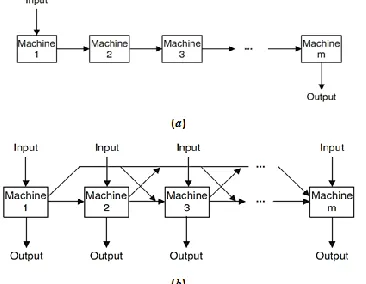
The shop contains m different machines, and each job consists of m operations, each of which requires a different machine. The flow shop is characterized by a flow of work that is unidirectional. When machines are numbered, so that if the jth operation of any job precedes its kth operation, then the machine required by the jth operation has a lower number than the machine required by the kth operation. The machines in a flow shop are numbered 1, 2, ..., m; and the operation of jobi correspondingly are numbered (i,1),(i,2),...,(i,m). Each job can be treated as if it has exactly m operations, in case there is jobi; for some i has fewer than m operations, the corresponding processing times can be set to zero [9]. The flow of work in pure flow shop is shown in Figure 1 (a), and (b) shows the flow of work in a more general one.
Fig. 1. (a) The flow of work in pure flow shop, (b) the flow of work in a more general flow shop
B. Flow shop Representation
Flow shop scheduling is represented by a disjunctive graph [2] [13], which is generally described as graph G = (V, C, D); with V is a set of nodes representing all operations of all jobs, C is set of directed conjunctive arc representing precedence relation among jobs (job precedence), and D is set of undirected disjunctive arc relating operations processed in the same machine. Figure 2 shows an example of disjunctive graph for flow shop scheduling problem with 4 jobs and 4
machines.
Fig. 2. Example of disjunctive graph for flow shop scheduling problem with 4 jobs and 4 machines
As scheduling problems in general, their solution (i.e., schedules) can be represented by Gantt chart [9] [13]. The chart is shown in Figure 3.
Fig. 3. Example of Gantt chart for solution representation of flow shop scheduling
Flow shop scheduling problem optimizing makespan can be detonated with triplet ; where describes machine
environment, β is a field for constraint and characteristic process, and is the problem objective – minimize
makespan.
Makespan ( ) of flow shop scheduling is amount of
time of the last job in a machine had been processed. Therefore, if is completion time of , makespan for flow shop scheduling with machines and jobs is defined as
{ }. Hence, the definition of
indicates that the smaller makespan value of schedule the more optimal the solution.
C. Intelligent water drop
The IWD algorithm was first time introduced in 2007 by Hamed Shah-Hosseini. It is built by two properties : , the speed of algorithm; and , the amount of soil is carried by algorithm. These properties may change during its life time.
D. Intelligent water drop algorithm
condition of termination is achieved. End of each iteration is indicated by the completion of solution generation of all IWD. At the end of each iteration, the best iteration solution ( ) is
chosen, and it is used to update the best solution ( ). The
number of soil on edges that generates will be subtracted
based on quality of the solution, and the algorithm will perform next iteration with new values of parameters. The algorithm will stop when either the maximum iteration or
with the required quality had been achieved.
The IWD algorithm has two kinds of parameters: statical parameter, one that has constant value during algorithm is running; and dynamical parameter, one that its value will be reinitialized at the end of each iteration. The steps of IWD algorithm can be described as follows.
1) Initialization of statical parameters, such as graph ( ), the best total solution initialized by the worst value,
number of iteration determined by user, iteration
counter variable initialized by 0. The number of
water drop initialized by a positive integer value,
usually equal to number of node in graph of problem. Parameters , , and are used to update velocity variable of IWD. Parameters , , and are used to update variable of IWD. Parameters n = 0.9 is used to update local variable of IWD, and is used to update
global variable of IWD. Parameter used to initialized for each path between two nodes i and j, ( ) . Initialization of for each is done by giving a value corresponds tothe value of parameter, while the values of and parameters are determined by user.
2) Initialization of dynamical parameters. Every has ( ) that records nodes that had already been visited by that , ( ) is initialized by empty set . Besides, it also has that is initialized by a value corresponds to , and soil for each is initialized by 0.
3) Randomly distribution of all of to nodes in graph as the first nodes that will be visited by that .
4) Insertion of first node for every to corresponding ( ) of that .
5) Repetition of steps from 5.a) through 5.d) for every until all nodes had been visited.
a. For is currently in , choose that satisfy constraints of the problem, and hasnot been in VC(IWD) with probability
( ) ( ( ))
∑ ( ) ( ( )), with ( ( ))
( ( )), and ( ( )) ( ) if
( )( ( )) , and ( ( ))
( ) ( )( ( )) for others. Node
(i.e., ) is then inserted into ( ).
b. For every moving from to , variabel ( ) is updated with (according to) (
) ( )
( ).
c. Computation of obtained by from path
between and travesed, i.e., ( ) according to the formula
( ) ( ( )) where ( ( )) ( )
( ) and ( ) is
determined heuristic undesirability.
d. Updating ( ) from path connecting to , and also (one that is brought by )
according to formula ( ) ( ) ( ) ( ) and formula
( ).
6) Selecting the best iteration solution among all
solutions obtained by according to the formula
( ), where q is quality function
of solution.
7) Updating on selected path by the best iteration solution according to the formula ( )
( ) ( )
( ) ,
where is the number of nodes in .
8) Updating the best total solution for this iteration,
according to if ( ) ( ),
otherwise.
9) Updating number of iteration, , if
, then return to step 2.
10) The IWD algorithm terminates with the best solution .
E. An adjusted IWD for Flow shop scheduling problem In order to conveniently implement IWD algrithm to find solution for flow shop scheduling problem, first is a certain number of adjustments performed. The adjusted IWD algorithm creates a number of intelligent water drops , places them on a number of points (or nodes) to start per-forming their flows and building the solution of the problem as ’s are flowing. Therefore, the problem to be solved must be represented by a graph. The flow shop scheduling problem to be solved by IWD algorithm is a flow shop with m machines and n jobs in order to minimize makespan.
The schedule is represented as a digraph ( ) with is set of nodes ( ) – operation of job in machine , and is a set of edges as a union of disjunctive arcand conjunctive arc of flow shop scheduling denoted by ( ). Adjusted IWD algorithm constructs the solution for flow shop scheduling problem in certain number of stages, the solution is constructed by every created , so that one will construct one schedule. Every flows through every node in the problems’ digraph, and the flows of to a node indicates that operation represented by that node is running.
1) Adding statical parameter denotes the number of created , and initialized by number of jobs in scheduling, . Only nodes that represent first operation of each job ( ) will be processed at the first time, and will be considered as initial nodes.
2) Adding statical parameter of processing time ( ), for operation ( ).
3) Adding statical parameter will store the list of ( ) of the best total solution.
4) Adding dynamical parameter and for every
used to compute makespan of schedule built by every . tmachine records time where machine finish processing, while records time where job finish being processed. The initial value ofboth and
are zero.
5) Adding dynamical parameter stage for every and every job, used to store machine number where every job the last time being processed. Besides, stage parameter also used to determined which nodes are visitable by every during building the solution. The initial value of stage for each job are initialized by 0 – all of jobs have not been processed, and the value will be updated by last machine number where the corresponding job being processed at the last time.
6) For step 3 of IWD (original) algorithm, the distribution of to a number of nodes did not perform randomly. Each of will be placed at every first operation node of each job.
7) Adding step to step 4 of IWD (original) algorithm.This additional step updates values of , and stage parameters for every . For every node ( ) that has just been visited, ( ) ( ), ( ) ( ),
and ( ) .
8) At the step 5.1 of IWD (original) algorithm, the selection of next visited nodes by must meet the job precedence rule in flow shop scheduling. The following are the rules for selecting those nodes.
node ( ), if ( ) ,
node ( ), if ( ) , for . 9) First condition denotes the nodes of first operation every
job that has not been in ( ) list. First operation (the operation in machine 1) of each job can be performed any time. This means that these nodes can be visited by providing they are not in the list of ( ). While the second makes sure thatjob precedence in flow shop scheduling is satisfied – operations of job must done sequentially, starting from operation ( ), then ( ), etc. Hence, operation ( ) can be done only if operation ( ) had been done. In IWD algorithm, this means that nodes ( ) can be visited only if node ( ) had been visited (or already been in ( ) list). When a job has means the job is last time processed in machine , then nodes representing this job will not be put in the list of next visitable nodes.
10) Heuristic undesirability ( ) for flow shop scheduling is assigned by the same value as idle time of machines in this scheduling process. This value measures how
big the unwillingness of not to move from one node to the next. The value of machine idle time is chosen as the value of , since the value of will be used to determine time required by IWD to flow to the next visited node, and this time value must be proportional with its value. Hence, the bigger value of idle time (or ) the longer time required by IWD to move from a node. For an IWD that will move from node ( ) to node ( ), the value of can be determined by taking the value of idle time of machine – how long this machine should be idle until node ( ) is visited. The value of for that move from node ( ) to node ( ) is given by : ( )( ) ( )
( ), if and ( ) ( ), and
( )( ) , for others. The value of will be zero if , it means that the next node is an operation that will be processed in machine 1 (first machine). It happened since any operation processed in the first machine will immediately be started providing the previous operation for this machine had been done, so that the first machines will never have idle time. While idle time of other machines are computed by comparing the values of ( ) and ( ). If
( ) ( ) – has not been completely
processed in machine ( ) when machine is ready to process , then according to job precedence in the flow shop scheduling, operation ( ) will start once had been processed in machine . In this case, machine must be idle until had been done with machine ( ) – the value of idle time of machine is equal to the last time being processed in machine ( ) minus time of machine . If ( )
( ), then had been processed in machine
( ), when machine ready to process , then is immediately processed in machine and the value of idle time of machine is equal to zeroHeuristic undesirability (HUD) for flow shop scheduling is assigned by the same value as idle time of machines in this scheduling process. This value measures how big the unwillingness of not to move from one node to the next. The value of machine idle time is chosen as the value of , since the value of will be used to determine time required by IWD to flow to the next visitednode, and this time value must be proportional with its value. Hence, the bigger value of idle time (or ) the longer time required by to move from a node. For an IWD that will move from node ( ) to node ( ), the value of can be determined by taking the value of idle time of machine – how long this machine should be idle until node ( ) is visited. The value of for that move from node ( ) to node ( ) is given by : ( )( ) ( )
( ), if and ( ) ( ), and
the first machine will immediately be started providing the previous operation for this machine had been done, so that the first machines will never have idle time. While idle time of other machines are computed by comparing the values of ( ) and . If
( ) ( ), then has not been
completely processed in machine ( ) when machine is ready to process , then according to job precedence in the flow shop scheduling, operation ( ) will start once had been processed in machine ( ). In this case, machine must be idle until had been done with machine ( ) – the value of idle time of machine is equal to the last time being processed in machine ( ) minus time of machine .
If ( ) ( ) – had been processed in
machine ( ), when machine ready to process , then is immediately processed in machine and the value of idle time of machine is equal to zero.
11) Adding new step 5.5 to step 5 of IWD (original) algorithm. It is required to update values of ; , and . For that moves from node ( ) to
node ( ), updating those values was done in accordance with :
( ) ( ) ( ), if and
( ) { ( ) ( )} ( ),
if ,
( ) ( ),
( ) ( )
12) The best total solution , and the best iteration solution of IWD algorithm for flow shop scheduling problem is of built schedule that is computed by ( ), where is number of
machines. Once the solution was built, was computed for every built schedule whose value is
( ) – the last machine perform processing.
13) Quality function () is a minimal function. Therefore, the formula ( ) will produce the minimal value of makespan. In accordance with the objective of scheduling, either or the solution is makespan with minimal value.
14) Adding step to reinitialize ( ) as done in the implementation of IWD algorithm for traveling salesman problem [7]. Based on characteristic of the flow shop scheduling, reinitialization is done every 20 iterations, according to: ( ) for any ( ) , and ( ) for others. After
20 iterations, soil of all paths are reset to except one of paths that built best total solution. For these paths, is initialized by the value of times 0.001. This multiplication is required to make paths of best total solution has with fewer value than one of other paths, so that these paths tend to be selected by ’s as the flowing paths in the next iteration.
15) Termination criteria is defined by the maximum iteration.
Fig. 4. Flowchart of the adjusted IWD Algorithm for Flow shop scheduling
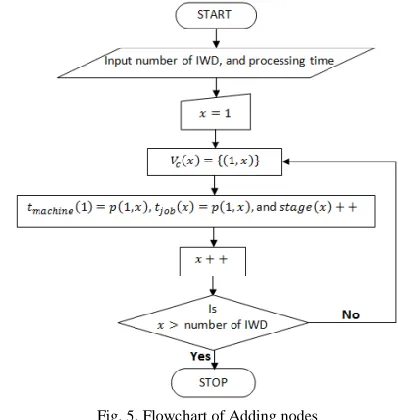
Considering a number of adjustments made to IWD algorithm mentioned above, so that the flowchart of the complete adjusted IWD algorithm can be described in Figure 4. Subsequently, Figure 6 and Figure 5 respectively shows the flowcharts of two dominant subprocesses of adjusted IWD algorithm in Figure 4 with (*) and (**) marks.
Fig. 5. Flowchart of Adding nodes
( ) ( )), and their , and . The process will terminate whenever is greater than the number of .
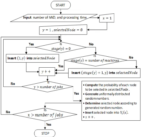
Fig. 6. Flowchart of Selecting and Inserting nodes
The beginning process for selecting the nodes is similar to the one for adding nodes. For each , however, is performed several steps, such as selecting the node to be visited next, possibility of the node being selected, generatingrandom number and determinating the selected node from this generated random numbers, and the possibility of each node. Finally, inserting the selected node into ( ). If all steps mentioned above had been done in all s, the process terminates.
IV. EXPERIMENTATIONSANDRESULTS In order to test the algorithm, a program was developed in Java using an application Netbeans IDE 6.9.1. The program was run on a computer with hardware specifications: processorIntel Pentium Dual-Core CPU E6600 3.06GHz, memory 4GB DDR III, and Graphic card Intel G41 Express Chipset, and the software specifications: Windows 8 (6.2) 32-bit (Build 9200) and Java Runtime Environment Version 7 update 45. Figure 7 shows an example of processing time data of each job in every machine (in this example, there are 20 jobs and 5 machines).
Fig. 7. An example of processing time data for 20 jobs and 5 machnes
The values of processing time can be either manually inputed or randomly generated with selected random number distribution. An illustration of this inputing stage is shown in Figure 8.
Figure 8: An illustration of inputing stage
While Figure 9 shows an example of program testing result. For simplicity reason, it uses input with 3 jobs and 2 machines (small number of job and machines).
Further testing was performed by varying the input values of scheduling – the number of machines, the number of jobs, and their processing time. In order to capable of comparing the testing result of adjusted IWD algorithm with those of results obtained from implementation of ant colony algorithm in flow shop scheduling problem done by Yagmahan and Yenisey (2010) – MOACSA (Multi-Objective Ant Colony System Algorithm), testing was conducted by dataset from Taillard (1993).
Fig. 9. An example of program testing result
To keep a fairness of comparison, parameter values of the adjusted IWD algorithm are specified similarly with ones specified in the research of IWD in TSP done by Hamed Shah-Hosseini (2009); i.e., ; ; ; ;
; ; ; ; ; and . All of dataset used in the testing was downloaded from http://mistic.heig-vd.ch/taillard/ problems.dir/ordonnancement.dir/ordonnancement.html.
is shown in Table I.
Table I
The comparison of makespans resulted by MOACSA and by adjusted IWD algorithm for Flow shop scheduling
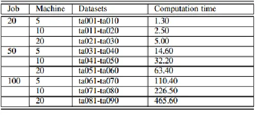
In addition, times required by Adjusted IWD algorithm to find a solution (i.e., computation time) for various pairs of job number and machine number is shown in Table II.
Table II
The computation time of Adjusted IWD algorithm for flow shop scheduling
V. CONCLUSION
The IWD algorithm introduced by Hamed Shah-Hosseini (2009) was successfully implemented for solving flow shop scheduling problem by adjusting a certain number of steps (i.e., adding both statical and dynamical parameters, defining the updating mechanism for parameters , , and
, etc.). Based on the testing results of the adjusted IWD algorithm (especially of scheduling), and the comparison with ones obtained by ant colony algorithm for flow shop scheduling shown in Table I, on average the adjusted IWD algorithm gave better solution (more optimal) than ant colony algorithm had.
REFERENCES
[1] A., Rabanimotlagh, 2011. An Efficient Ant Colony Optimi-zation Algorithm for Multiobjective Flow Shop Schedu-ling Problem. WASET, 51, 127-133.
[2] B., Yagmahan, and M.M., Yenisey, 2008. Ant Colony Optimization for Multi-Objective Flow Shop Scheduling Problem. Computers and Industrial Engineering, 54, 411-420.
[3] B., Yagmahan, and M.M., Yenisey, 2010. A Multiobjective Ant Colony System Algorithm for Flow Shop Scheduling Problem. ESWA, 37, 1361-1368.
[4] C., Rajendran, and H., Ziegler, 2004. Ant-Colony Algori-thms for Permutation Flowshop Scheduling to Minimize Makespan/Total Flowtime of Jobs. EJOR, 155, 426-438.
[5] E., Taillard, 1993. Benchmark for Basic Scheduling Pro-blems. EJOR, 64, 278-285.
[6] H., Boukef, M. Benrejeb, and P., Borne, 2007. A Proposed Genetic Algorithm Coding for Flow-Shop Scheduling Problems. IJCCC, 3, II, 229-240.
[7] H., Shah-Hosseini, 2007. Problem Solving by Intelligent Water Drops. IEEE Congress on Evolutionary Computa-tion, Singapore. [8] H., Shah-Hosseini, 2009. The Intelligent Water Drops Algorithm:
A Nature-Inspired Swarm-Based Optimiza-tion Algorithm. IJBIC, 1/2, 1, 71-79.
[9] K.R., Baker, and D., Trietsch, 2009. Principles of Sequencing and Scheduling. John Wiley Sons, Inc., New Jersey.
[10] M.F., Tasgetiren, Q.K., Pan, P.N., Sganthan, and A.H.L., Chen, 2011. A Discrete Artificial Bee Colony Algorithm for the Total Flowtime Minimization in Permutation Flow Shops. Information Sciences, 181, 3459-3475.
[11] M.H.A., Ashkezari, N.S., Pour, and H.M., Andargoli, 2012. An Ant Colony System for Solving Fuzzy Flow Shop Scheduling Problem. International Journal of Engineering and Technology, 1, 2, 44-57. [12] M.L., Pinedo, 2008. Scheduling Theory, Algorithms, and Systems.
3rd edition, Springer, New York.
[13] P., Bruker, 2007. Scheduling Algorithms. 5th edition, Springer, 5th
edition, New York.