http://www.sciencepublishinggroup.com/j/ijepe doi: 10.11648/j.ijepe.20160505.11
ISSN: 2326-957X (Print); ISSN: 2326-960X (Online)
Optimal Network Reconfiguration and Distributed
Generation Placement in Distribution System Using a
Hybrid Algorithm
Mohammad Ali Hormozi, Mohammad Barghi Jahromi, Gholamreza Nasiri
Fars Regional Electrical Company, Shiraz, Iran
Email address:
To cite this article:
Mohammad Ali Hormozi, Mohammad Barghi Jahromi, Gholamreza Nasiri. Optimal Network Reconfiguration and Distributed Generation Placement in Distribution System Using a Hybrid Algorithm. International Journal of Energy and Power Engineering.
Vol. 5, No. 5, 2016, pp. 163-170. doi: 10.11648/j.ijepe.20160505.11
Received: August 26, 2016; Accepted: September 13, 2016; Published: October 19, 2016
Abstract:
In this paper a method for solving optimal distribution network reconfiguration and optimal placement distributed generation (DG) with the objective of reducing power losses and improving voltage profile with the least amount of time using a combination of various techniques is offered. In the proposed method, first, a meta-heuristic algorithm (MHA) is used to solve the problem of optimal DG placement. The search space for using this technique has been reduced to the optimal scale which is why this technique is accurate and quick. After solving optimal DG placement using the abovementioned technique, a binary particular swarm optimization algorithm (BPSO) is presented for solving the network reconfiguration. In fact, by reducing the search space, the speed of the technique for solving the problem is improved. The proposed technique has been implemented with different scenarios on IEEE 33- and 69-node test systems. The comparison of the results with those of other methods indicates the effectiveness of this technique.Keywords:
Distribution Network Reconfiguration, Distributed Generation, Hybrid Algorithm, Meta-Heuristic Algorithm, Binary Particular Swarm Optimization Algorithm, Power Loss1.
Introduction
Distributed Generation plays an important role in electricity markets and power systems. Installation of DG on distribution feeders can have a significant impact on power system operation and control [1]. DG can be fitted with different strategies in the power network. For example, reducing power losses, cost reduction peak load, improving voltage profile or system reliability, all depend on the location and size of the DG [2]. Since selection of the best locations and sizes of DG units is also a complex combinatorial optimization problem, many methods are proposed in this area in the recent past [3]. Wang and Nehrir [4] proposed an analytical method to determine optimal location to place a DG in distribution system for power loss minimization. Celli et al. [5] presented a multi-objective algorithm using GA for sitting and sizing of DG in distribution system.
Optimal network reconfiguration is, in fact, the best network configuration among all existing configurations in
example, genetic algorithms [10], neural networks [11], simulated annealing [12], swarm optimization [13], ant colonies [14]. In [3], authors have dealt with network reconfiguration and DG placement simultaneously using Harmony Search Algorithm (HSA) based only on minimization of power losses. In [15] using fireworks optimization algorithm for solving the distribution system network, reconfiguration, together with DG placement, for the problem of power loss minimization and voltage stability enhancement has been done.
The proposed technique combines the BPSO algorithm for solving the optimal network reconfiguration with MHA algorithm for solving the optimal placement of DG. The proposed technique has been validated on two standard IEEE 33- and 69-node test systems, and the simulated results were
compared with the results of other techniques available [3-15] in the literature to assess the performance and effectiveness of the proposed method.
This paper is organized as follows: Section 2 gives the problem formulation, Section 3 overview of the hybrid algorithm and the proposed method, Section 4 presents results, and Section 5 outlines conclusions.
2. Problem Formulation
2.1. Power Flow Equations
Power flows in a distribution system are computed by the following set of equations [16]:
= − , − = −| | + + | | − (1)
= − , − = −| | + + | | − | | − | | − (2)
| | = | | + | | + − 2 + = | | + | | + + | | − 2 + + | | (3)
The power loss in the line section connecting nodes and + 1 may be computed as , + 1 = ∗ "# $| | % (4)
The total power loss of the system is determined by the summation of losses in all the line section, which is given as &, = ∑(*) , + 1 (5)
2.2. Power Loss Using Network Reconfiguration The power loss of a line section connecting nodes between and + 1 after reconfiguration of network can be computed as +, , + 1 = ∗ -#./0 $./0 1 ./01 2 (6)
The total power loss after reconfiguration of the system is determined by the summation of losses in all the line section, which is given as &,+, = ∑(*) +, , + 1 (7)
2.3. Objective Function of the Problem The objective function of the problem is formulated to minimize the power loss reduction in distributed system, which is given by 45654578 9 1 = 456. ;#<,)=>>?@ #<,)=>>A (8)
45654578 9 2 = 456. ;#<,)=>>./0 B A (9)
2.4. Constraints of the Problem 1) Apparent Power flow through any distribution feeder must comply with the thermal capacity of line, that is, |C | ≤ 1C ,EFG1 (10)
2) Node voltages and line currents limits: EHI ≤ | +,| ≤ EFG (11)
EHI≤ 1 JK1 ≤ EFG (12)
1L ,+, 1 ≤ 1L , ,EFG1 (13)
1LJK, 1 ≤ 1L , ,EFG1 (14)
3) Power conservation limits:
MNO+ ∑(*P JK, = ∑(*) , + 1 + ∑(*R FQ,
(15) 4) DG capacity limit:
&JK ≤ #STU (16) 5) DG location limit:
The search space for each DG unit location limited to four nodes candidate:
VW = VJK∗ 4 YZ6[5[Z\8 (17)
6) The radial constraint is verified by using incidence matrix ] .
3. The Proposed Method by Hybrid
Algorithm
3.1. Objective Function of the Problem
A hybrid algorithm is an algorithm that combines two or more other algorithms that solve the same problem, either choosing one (depending on the data), or switching between them over the course of the algorithm. This is generally done to combine desired features of each, so that the overall algorithm is better than the individual components. In [17], network reconfiguration and DG placement simultaneously using novel hybrid method of meta-heuristic and heuristic algorithms in order to boost robustness and shorten the computational runtime to achieve network minimum loss configuration in the presence of DGs. In [18], Optimal reconfiguration using a combination of Tabu Search (TS) and Branch Exchange (BE) in order to minimize energy loss. 3.2. MHA for Solving Optimal DG Placement
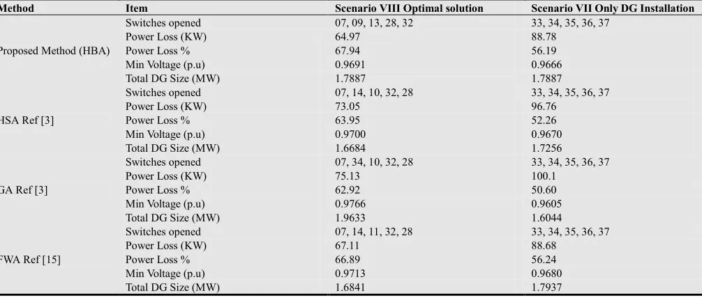
The stages of the proposed meta-heuristic algorithm for DG placement which does not need much time to be solved consist of the following:
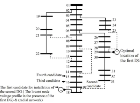
Step 1: Close all tie switches in the network. (Ring network)
Step 2: We find the node that has the least voltage profile and select it as the first candidate for installing DG. Are we considering the initial optimal value of this DG, 1/3 of the active power of the network and we put it in the network. Then, by obtaining power flow in the network, we calculate network loss. Now we limit the next candidate for installing this DG to one to three nodes before the selected node. By installing this DG on these nodes, the node that has the least power loss is the suitable one for installing this DG (Figure 1).
Step 3: For adding another DG to the network, first, turn the network to the normal condition (Radial network). Second, we act as in step 2 by considering the presence of the first DG in the network and calculating power flow with the change that the value of the second DG is 1/3 of the first DG. In the same way we consider the value of the next DG 1/3 of the previous DG. The results of simulation show that the 1/3 estimation is quite optimal. The next DG placements are obtained in the presence of the first DG as in Figure 2. Step 4: After we have had enough optimal DG placements
in the network, we do the reconfiguration in the presence of all the DGs which leads to a quite optimal result. Accordingly, by limiting the search space for finding the optimal placement and estimating the optimal value of the DG there is no need to spend a lot of time for solving the problem and the simulation results show that it is quite optimal.
Fig. 1. Optimum location for installation of the first DG.
Fig. 2. Optimum location for installation of the next DG.
3.3. BPSO for Solving Network Reconfiguration
The parameters of BPSO algorithm used in the simulation of network are Number of iterations VgFG= 3, Number of runs ViNI=10, Inertia weight jEFG 0.9, jEHI 0.4, and Acceleration constants l, 2. The search space was optimally reduced which leads to high accuracy and fast performance of this technique. Indeed, by removing the switches that are not effective in solving optimization problem the performance of this technique improves. By using the 33- node system the way to find the optimal search space is shown.
Step 1: By closing all tie switches, the network will become multi loop. Now to specify any loop in the network, one should note that each tie switch must belong to a loop. In Figure 3, each loop is shown with different geometric shapes.
Step 2: Removing the branches that do not belong to any of the loops. In Figures 3, they are not shown with any geometric shapes.
Step 3: Removing the branch of the loops which does not share with other loops.
a) If a desired branch has more than three switches, it will be removed.
part that has the minimum number of switches will be removed. If the tie switch does not share with another loop, it will be removed itself.
Step 4: After the network has been simplified we go to step 2 and do the simplification again bearing in mind that in repeating the process no tie switch will be removed (Figure 4).
Fig. 3. Search space of the 33-node system.
Fig. 4. Optimum search space of the 33- node system.
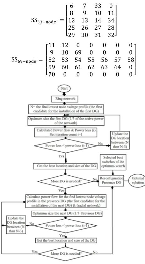
Therefore, with the proposed method, the search space in the 33-node system is reduced from 37 switches to 19 switches and it is reduced in the 69-node system from 73 switches to 19 switches. So the optimal search space to find the suitable switches for opening or closing in the network is as follows with each row of the matrix representing each loop in the network:
SSnnopqrs =
t u u u
v68 7 339 10 110 12 13 14 34 25 26 27 28 29 30 31 32{|
| | }
SS~•opqrs
t u u u
v11 129 10 690 00 00 00 00 52 53 54 55 56 57 58
59 60 61 62 63 64 0
70 0 0 0 0 0 0 {|
| | }
Fig. 5. Flow chart of the proposed technique HBA.
4. Simulation Results
In order to demonstrate the effectiveness of the proposed technique using HBA, it is applied to two test systems consisting of 33 and 69 node. In the simulation of network, eight scenarios are considered to analyze the superiority of the proposed technique. The results simulated are compared with the results of other techniques such as FWA [15] and HSA [3] and GA [3] to assess the performance and effectiveness of the proposed technique.
Scenario I: The system is without reconfiguration and DG (Base case);
Scenario II: The system is with reconfiguration and without DG unit;
Scenario III: The system is without reconfiguration and with installation of the first DG unit; Scenario IV: The system is with reconfiguration and
installation of the first DG unit;
with installation of the two DG units; Scenario VI: The system is with reconfiguration and
installation of the two DG units;
Scenario VII: The system is without reconfiguration and with installation of the three DG units; Scenario VIII:The system is with reconfiguration and
installation of the three DG units (Optimal solution).
All scenarios are programmed in MATLAB, and simulations are carried on a computer with Pentium IV, 1.8 GHz, 2 GB RAM.
4.1. 33-Node Test System
The line, load and tie line data of this test system are taken from [19]. The normally closed sectionalize switches are 1–32 and the open tie switches are 33–37. The single line diagram of 33-node system with the loops formed corresponding to each tie switch is shown in Fig. 1. The total real and reactive power loads of the system are 3715 KW and 2300 KVAr, respectively. The performance of the proposed method at nominal load level is presented in Table 1. The total power loss (kW) at nominal load condition is reduced from 202.67 to 64.96 in
scenario VIII respectively. In order to illustrate the performance of the proposed technique, the performance of HBA is compared with the results of FWA [15], HSA [3] and GA [3] available in the literature and is presented in Table 2.
Fig. 6. Voltage profile of 33-node system.
Table 1. Results of 33-node system.
Switches Opened Power Loss (KW) Min Voltage (p.u) Size of DG in MW (Location) CPU Time (s)
Scenario I 33, 34, 35, 36, 37 202.67 0.9131 - -
Scenario II 07, 09, 14, 28, 32 139.98 0.9412 - 1.969
Scenario III 33, 34, 35, 36, 37 120.63 0.9295 1.23830 (29) 0.003
Scenario IV 07, 09, 14, 28, 32 89.81 0.9479 1. 23830 (29) 2.532
Scenario V 33, 34, 35, 36, 37 93.5 0.9558 1. 23830 (29) 0.01
0.41278 (15)
Scenario VI 07, 09, 13, 28, 32 69.64 0.9662 1. 23830 (29) 3.043
0.41278 (15)
Scenario VII 33, 34, 35, 36, 37 88.78 0.9666
1. 23830 (29)
0.02 0.41278 (15)
0.13759 (18)
Scenario VIII 07, 09, 13, 28, 32 64.97 0.9691
1. 23830 (29)
3.552 0.41278 (15)
0.13759 (18)
Table 2. Comparison of simulation results of 33-node system.
Method Item Scenario VIII Optimal solution Scenario VII Only DG Installation
Proposed Method (HBA)
Switches opened 07, 09, 13, 28, 32 33, 34, 35, 36, 37
Power Loss (KW) 64.97 88.78
Power Loss % 67.94 56.19
Min Voltage (p.u) 0.9691 0.9666
Total DG Size (MW) 1.7887 1.7887
HSA Ref [3]
Switches opened 07, 14, 10, 32, 28 33, 34, 35, 36, 37
Power Loss (KW) 73.05 96.76
Power Loss % 63.95 52.26
Min Voltage (p.u) 0.9700 0.9670
Total DG Size (MW) 1.6684 1.7256
GA Ref [3]
Switches opened 07, 34, 10, 32, 28 33, 34, 35, 36, 37
Power Loss (KW) 75.13 100.1
Power Loss % 62.92 50.60
Min Voltage (p.u) 0.9766 0.9605
Total DG Size (MW) 1.9633 1.6044
FWA Ref [15]
Switches opened 07, 14, 11, 32, 28 33, 34, 35, 36, 37
Power Loss (KW) 67.11 88.68
Power Loss % 66.89 56.24
Min Voltage (p.u) 0.9713 0.9680
Total DG Size (MW) 1.6841 1.7937
0 5 10 15 20 25 30 35
0.91 0.92 0.93 0.94 0.95 0.96 0.97 0.98 0.99 1
V
o
lt
ag
e
M
ag
n
it
u
d
e
(p
.u
)
Node Number
Voltage Profile of 33-Node System at Nominal Load
4.2. 69-Node Test System
This is a 69-node large scale radial distribution system with 68 sectionalizing and five tie switches. Configuration, line, load, and tie line data are taken from [20]. Total system loads for base configuration are 3802.19 KW and 2694,06 KVAr. The sectionalizing switches are labeled from 1 to 68 and tie
switches from 69 to 73, respectively.
Similar to 33 node test system, this test system is also simulated for eight scenarios at one load level and the results are presented in Table 3. The total power loss (KW) at nominal load condition is reduced from 224.96 to 38.36 in scenario VIII respectively.
Table 3. Results of 69-node system.
Switches Opened Power Loss (KW) Min Voltage (p.u) Size of DG in MW (Location) CPU Time (s)
Scenario I 69, 70, 71, 72, 73 224.97 0.9091 - -
Scenario II 12, 58, 61, 69, 70 98.79 0.9494 - 2.556
Scenario III 69, 70, 71, 72, 73 96.58 0.9578 1.2673 (61) 0.001
Scenario IV 12, 55, 64, 69, 70 50.54 0.967 1.2673 (61) 3.488
Scenario V 69, 70, 71, 72, 73 83.95 0.9672 1.2673 (61) 0.008
0.42243 (64)
Scenario VI 12, 56, 61, 69, 70 39.49 0.9776 1. 2673 (61) 4.372
0.42243 (64)
Scenario VII 69, 70, 71, 72, 73 78.1 0.9743
1. 2673 (61)
0.01 0.42243 (64)
0.14081 (24)
Scenario VIII 12, 57, 61, 69, 70 38.36 0.9777
1. 2673 (61)
5.26 0.42243 (64)
0.14081 (24)
Fig. 7. Voltage profile of 69-node system.
The performance of HBA on 69-node system is also compared with the results of FWA and HAS and GA methods similar to 33-node system, and the results are presented in Table 4.
0 10 20 30 40 50 60 70
0.9 0.91 0.92 0.93 0.94 0.95 0.96 0.97 0.98 0.99 1
V
o
lt
ag
e
M
ag
n
it
u
d
e
(p
.u
)
Node Number
Voltage Profile of 69-Node System at Nominal Load
Table 4. Comparison of simulation results of 69-node system.
Method Item Scenario VIII Optimal solution Scenario VII Only DG installation
Proposed Method (HBA)
Switches opened 12, 57, 61, 69, 70 69, 70, 71, 72, 73
Power Loss (KW) 38.36 78.10
Power Loss % 82.94 65.28
Min Voltage (p.u) 0.9777 0.9679
Total DG Size (MW) 1.8305 1.8305
HSA Ref [3]
Switches opened 69, 17, 13, 58, 61 69, 70, 71, 72, 73
Power Loss (KW) 40.03 86.77
Power Loss % 82.08 61.43
Min Voltage (p.u) 0.9736 0.9677
Total DG Size (MW) 1.8718 1.7732
GA Ref [3]
Switches opened 10, 15, 45, 55, 62 69, 70, 71, 72, 73
Power Loss (KW) 46.20 88.5
Power Loss % 73.38 60.66
Min Voltage (p.u) 0.9727 0.9687
Total DG Size (MW) 2.0292 1.9471
FWA Ref [15]
Switches opened 69, 70, 13, 55, 63 69, 70, 71, 72, 73
Power Loss (KW) 39.25 77.85
Power Loss % 82.55 65.39
Min Voltage (p.u) 0.9796 0.9740
Total DG Size (MW) 1.8182 1.8329
5. Conclusion
In this paper a hybrid algorithm for solving optimal distribution network reconfiguration and optimal DG placement with the objective of reducing power loss and improving voltage profile was presented. The first algorithm for solving optimal DG placement is to use a simple meta-heuristic algorithm (MHA) which estimates optimal places for installing DG and their value. The second algorithm for solving reconfiguration is a quick binary particular swarm optimization (BPSO) algorithm. The results obtained clearly
indicate that scenario VIII (DG installation with network reconfiguration) is found to be more effective in minimizing the power loss compared to the other scenarios considered. To show the efficiency of the proposed algorithm tested it on two 33- and 69-node systems. The results show the better performance of this method compared to genetic algorithm (GA), harmony search algorithm (HAS), and fireworks algorithm (FWA). Considering the simplicity and quick performance of this proposed algorithm, one can use it in intelligent networks with total load of less than 10 megavolt ampere and with any number of nodes in real time.
Nomenclature
Real power flowing out of node . Reactive power flowing out of node .
+, Real power flowing out of node after reconfiguration. +, Reactive power flowing out of node after reconfiguration.
Real load power at node + 1. Reactive load power at node + 1.
MNO Active power supplied by the substation.
FQ, Real power load at node .
JK, Real power supplied by DG at node .
C Apparent power flowing in the line section between nodes and + 1.
C,EFG Maximum power flow capacity limit of line section between nodes and + 1.
V Total number of lines sections in the system.
VI Total number of nodes in the system.
VW Number of candidate nodes for DG installation.
VJK Number of DG unit in the system.
] Node incidence matrix.
L,+, Current in line section between nodes and + 1 after reconfiguration.
LJK, Current in line section between nodes and + 1 after DG installation.
L, ,EFG Maximum current limit of line section between nodes and + 1.
Reactance of the line section between nodes and + 1.
, + 1 Loss in the line section connecting nodes and + 1.
&,€bee Total power loss of the feeder.
&,+, Total power loss of the feeder after reconfiguration
&,JK Total power loss of the feeder with DG.
Voltage at node .
+, Voltage at node after reconfiguration. JK Voltage at node after DG installation.
EFG Maximum node voltage at node . EHI Minimum node voltage at node .
Shunt admittance at any node .
&JK Total real power of the DG units.
CC(I Search space of the test system.
References
[1] N. S. Rau and Y. H. Wan, “Optimal location of resources in distributed planning”, IEEE Trans. Power Syst., Vol. 9, pp. 2014-2020, Nov. 1994.
[2] W. EI-hattam, M. M. A. Salma, “Distributed Generation Technologies, Definitions and Benefits” Elect. Power Syst. Res., Vol. 71, pp. 119-1283, 2004.
[3] R. Srinivasa Rao, K. Ravindra, K. Satish, and S. V. L. Narasimham, “Power Loss Minimization in Distribution System Using Network Reconfiguration in the Presence of Distributed Generation,” IEEE Trans. Power Syst., vol. 28, no. 1, pp. 317–325, Feb 2013.
[4] C. Wang and M. H. Nehrir, “Analytical approaches for optimal placement of distributed generation sources in power systems,” IEEE Trans. Power Syst., vol. 19, no. 4, pp. 2068–2076, Nov. 2004.
[5] G. Celli, E. Ghiani, S. Mocci, and F. Pilo, “A multi-objective evolutionary algorithm for the sizing and the sitting of distributed generation,” IEEE Trans. Power Syst., vol. 20, no. 2, pp. 750–757, May 2005.
[6] J. J. Young, K. J. Chul, Jin-O. Kim, J. O. Joong-Rin Shin, K. Y. Lee, An efficient simulated annealing algorithm for network reconfiguration in large-scale distribution systems, IEEE Trans. Power Del., vol. 17, no. 4, pp. 1070–1078, October. 2002. [7] S. K. Goswami and S. K. Basu, “A new algorithm for the
reconfiguration of distribution feeders for loss minimization,” IEEE Trans. Power Del., vol. 7, no. 3, pp. 1484–1491, July 1992.
[8] A. Merlin and H. Back, “Search for a minimal-loss operating spanning tree configuration in an urban power distribution system,”in Proc. 5th Power System Computation Conf. (PSCC), Cambridge, U.K., pp. 1–18, 1975.
[9] S. Civanlar, J. Grainger, H. Yin, and S. Lee, “Distribution feeder reconfiguration for loss reduction,” IEEE Trans. Power Del., vol. 3, no. 3, pp. 1217–1223, Jul. 1988.
[10] K. Nara, A. Shiose, M. Kitagawa, and T. Ishihara, “Implementation of genetic algorithm for distribution systems loss minimum reconfiguration,” IEEE Trans. Power Syst., vol. 7, no. 3, pp. 1044–1051, August 1992.
[11] H. Kim, Y. Ko, and K. H. Jung, “Artificial neural networks based feeder reconfiguration for loss reduction in distribution systems,” IEEE Trans. Power Del., vol. 8, no. 3, pp. 1356– 1366, July 1993.
[12] H. C. Chang and C. C. Kuo, “Network reconfiguration in distribution system is using simulated annealing,” Elect. Power Syst. Res., vol. 29, pp. 227–238, May 1994.
[13] J. Kennedy and R. Eberhart, “A discrete binary version of the particle swarm algorithm,” Proc. IEEE Int. Conf. on Systems, Man, and Cybernetics (SMC 97), vol. 5, pp. 4104–4109, October 1997.
[14] C. T. Su, C. F. Chang and J.-P. Chiou, “Distribution network reconfiguration for loss reduction by ant colony search algorithm,” Elect. Power Syst. Res., vol. 75, pp. 190–199, August 2005.
[15] A. Mohamed Imran, M. Kowsalya, D. P. Kothari “A novel integration technique for optimal network reconfiguration and distributed generation placement in power distribution network,” Electr Power Energy Syst., vol. 63, pp. 461–472, 2014
[16] R. Srinivasa Rao, S. V. L. Narasimham, M. R. Raju, and A. Srinivasa Rao,“Optimal network reconfiguration of large-scale distribution system using harmony search algorithm,” IEEE Trans. Power Syst., vol. 26, no. 3, pp. 1080–1088, Aug. 2011. [17] H. R. Esmaeilian, R. Fadaeinedjad, “Energy Loss Minimization
in Distribution Systems Utilizing an Enhanced Reconfiguration Method Integrating Distributed Generation,” IEEE Syst. J., IEEE, pp. 1-10, July. 2014.
[18] N. G. A. Hemdana, B. Deppec, M. Pielked, M. Kurrata, T. Schmedesd, E. Wiebene “Optimal reconfiguration of radial MV networks with load profiles in the presence of renewable energy based decentralized generation” Elect. Power Syst. Res., Vol. 116, pp. 355-366, November 2014.
[19] M. E. Baran and F. Wu, “Network reconfiguration in distribution system for loss reduction and load balancing,” IEEE Trans. Power Del., vol. 4, no. 2, pp. 1401–1407, Apr. 1989.
[20] J. S. Savier and D. Das, “Impact of network reconfiguration on loss allocation of radial distribution systems,” IEEE Trans. Power Del., vol. 2, no. 4, pp. 2473–2480, Oct. 2007.