http://www.sciencepublishinggroup.com/j/com doi: 10.11648/j.com.20170503.11
ISSN: 2328-5966 (Print); ISSN: 2328-5923 (Online)
Comparative Study of Least Square Methods for Tuning
CCIR Pathloss Model
Nnadi Nathaniel Chimaobi
1, Ifeanyi Chima Nnadi
1, Chibuzo Promise Nkwocha
21Department of Electrical/Electronic Engineering, Imo State Polytechnic, Umuagwo, Owerri, Nigeria 2
Department of Chemical Engineering, Federal University of Technology, Owerri (FUTO), Owerri, Nigeria
Email address:
[email protected] (N. N. Chimaobi)
To cite this article:
Nnadi Nathaniel Chimaobi, Ifeanyi Chima Nnadi, Chibuzo Promise Nkwocha. Comparative Study of Least Square Methods for Tuning CCIR Pathloss Model. Communications. Vol. 5, No. 3, 2017, pp. 19-23. doi: 10.11648/j.com.20170503.11
Received: MM DD, 2017; Accepted: MM DD, 2017; Published: June 14, 2017
Abstract:
Comparative study of two least square methods for tuning CCIR pathloss model is presented. The first model tuning approach is implemented by the addition or subtraction of the root mean square error (RMSE) based on whether the sum of errors is positive or negative. The second method is implemented by addition of a composition function of the residue to the original CCIR model pathloss prediction. The study is based on field measurement carried out in a suburban area for a GSM network in the 1800 MHz frequency band. The results show that the untuned CCIR model has a root mean square error (RMSE) of 17.33 dB and prediction accuracy of 85.33%. On the other hand, the pathloss predicted by the RMSE tuned CCIR model has RMSE of 4.09dB and prediction accuracy of 96.82% while the pathloss predicted by the composition function tuned CCIR model has RME of 2.15 dB and prediction accuracy of 98.39%. In all, both methods are effective in minimizing the error to within the acceptable value of less than 7 dB. However, the composition function approach has better pathloss prediction performance with smaller RMSE and higher prediction accuracy than the RMSE-based approach.Keywords:
Pathloss, Propagation Model, CCIR Model, Composition Function, Empirical Model, RMSE-Based Tuning Approach, Least Square Method1. Introduction
Pathloss models are mathematical expressions designed for predicting the expected pathloss that signal can experience in a given environment [1-6]. Pathloss prediction is particularly essential in wireless network communication systems for determining the network coverage area. Empirical pathloss models are the pathloss models that are developed based on empirical measurements conducted in a specific area [7-9]. Empirical pathloss models are limited in their ability to predict pathloss effectively in different environments other than the one where they are developed from [10-14]. As such, model tuning is normally used to modify the model parameters so as to improve on the its pathloss prediction performance [15-18]. In this paper, comparative study of two pathloss tuning approaches are presented. The two approaches are basically least square methods that use different correction factors to minimize the pathloss prediction error. In the first approach, the correction factor is the root mean square error (RMSE)
whereas in the second approach the correction factor is obtained by using a composition function that estimates the pathloss prediction error based on the current pathloss prediction. Particularly, in this paper, the CCIR pathloss model is considered for 1800MHz GSM network in a suburban area.
2. Methodology
2.1. CCIR Pathloss Model
The CCIR (Comit´e Inter-national des
Radio-Communication, now ITU-R) developed an empirical pathloss model that takes into account the varying degrees of urbanization. The CCIR model is given as follows [19-22]:
= + ∗ log − (1) where A and B are defined in the Okumura-Hata model with
= 69.55 + 26.16 ∗ log − 13.82 ∗ log ℎ" − ℎ (2)
= 44.9 − 6.55 ∗ log ℎ" (3)
ℎ = $1.1 ∗ log − 0.7' ∗ ℎ − $1.56 ∗ log − 0.8' (4)
Eq 4 is for small city, medium city, open area, rural area and suburban area. The parameter E accounts for the degree of urbanization and is given by;
E = 30 − 25log (5)
Where PB is the % of area covered by buildings
where E = 0 when the area is covered by approximately 16% buildings.
For Urban Area PB ≥ 16% and hence, E is set to 0 for urban area.
For Sub-Urban Area PB < 16% (typical PB =8%). For Rural Area PB < 16% (typical PB =3%). Where
f is the centre frequency f in MHz d is the link distance in km
ℎ is an antenna height-gain correction factor that depends upon the environment
150 MHz≤ f≤ 1000MHz 30m ≤ℎ" ≤ 200m 1m≤ ℎ ≤ 10 m 1 km ≤ d ≤ 20km
2.2. Model Optimization Process
The parameters of the CCIR pathloss model were adjusted (optimized) using least square algorithm to fit to measured data using the following process.
1)First, the residual (or error, () ) between measured pathloss, *+ ) and the CCIR model predicted pathloss , *+ ) is calculated for each location point, i.
() = *+ ) - , *+ ) (6)
2)Second, the RMSE is calculated based along with sum of errors, that is ∑ .()01 )0 ) /.
3)Thirdly, if ∑ .()01 )0 ) / < 0 then the optimised model is obtained by subtracting RMSE from each , *+ ) otherwise, if ∑ .()01 )0 ) / ≥ 0 the optimised model is obtained by adding RMSE to each , *+ ), as given in Eq 6 ; () = *+ ) - , *+ )
4)For the RMSE–based tuning, the tuned pathloss model is denoted as PL456789:7; where,
PL456789:7;= *+ ) + <=>
5)For the composition function –based tuning, the tuned pathloss model is denoted as PL?@489:7; and the composition function of residue is denoted as
() where,
PL A BCDEF= *+ ) + () (7)
where
() = K1 ( *+ )) +K2 (8) K1 and K2 are the tuning coefficients for the composition of function of residual given as () .
Essentially, () is a function the predicts the residue (that, is the prediction error) based on the pathloss predicted by the untuned CCIR model.
2.3. Received Signal Strength (RSS) and Spatial Data Collection and Processing
Samsung Galaxy S4 mobile phone with Cellmapper android and MyGPS applications installed is used to capture and store the Received Signal Strength (RSS) and spatial data (longitude,latitude and altitude) dataset. The RSS and spatial data d are captured in a suburban area for a 18000MHz GSM network. The RSS is converted to the measured pathloss (PL) using the formula [23-25]:
*+ = PBTS + GBTS + GMS – LFC – LAB – LCF – RSS(dBm) (9) where
PLG HI is the measured pathloss for each measurement location at a distance d (km)
RSS is the mean Received Signal Strength (RSS) in dBm, PBTS = Transmitter Power (dBm), GBTS = Transmitter Antenna Gain (dBi), GMS = receiver antenna gain (dBi), LFC = feeder cable and connector loss (dB), LAB = Antenna Body Loss (dB) and LCF = Combiner And Filter Loss (dB). The values of these parameters are given as [13] as: PBTS = 40 W = 46 dBm, GBTS = 18.15 dBi, GMS = 0 dBi, LFC = 3 dB, LAB = 3 dB, LCF = 4.7 dB. Hence,
*+ = 53.5 (dBm).– RSS(dBm) (10)
Again, the Haversine formula in Eq 11 is used to computer the distances (d) between each measurement point and the base station as follows;
= 2, UVsin XYZB[\YZB]
^ _
^
+ cos a cos a^ sin XYbDc[\YbDc^ ]_ ^
[
d (11)
LAT in Radians = ef8 gh ;ijkiil ∗ m. n^o (12)
LONG in Radians = ep:q gh ;ijkiil ∗ m. n^o (13)
Where
LAT1 and LAT2 are the latitude of the coordinates of point1 and point 2 respectively
LONG1 and LONG2 are the longitude of the coordinates of point1 and point 2 respectively
R = radius of the earth = 6371 km
d = the distance between the two coordinates
R varies from 6356.752km at the poles to 6378.137 km at the equator
The pathloss prediction performance measures for the CCIR model are defined as follows:
MSE = Vu [ 1v∑) 0 1) 0 w xyz{|x* ) − }|x*)~•x* ) w^€•(14)
ii) Then, the Prediction Accuracy (PA, %) based on mean absolute percentage deviation (MAPD) or Mean Absolute Percentage Error (MAPE) is calculated as follows:
PA = ƒ1 −1 „∑ …w†Y‡ˆ‰Š‹Œˆ• Ž\†Y•Œˆ•Ž•‘ˆ• Ž w
†Y‡ˆ‰Š‹Œˆ• Ž …
)01
)0 ’“ * 100% (15)
3. Results and Discussions
The field measured distance, received signal strength (RSSI) and pathloss (PLm) are given in Table 1. The link budget equation, *+ = 53.5 (dBm) – RSS(dBm) is used to obtain the measured pathloss (PLm) whereas Haversine formula is used to obtain the distance between the GSM base station and each of the measurement point, where the longitude 1 and latitude 1 are that of the GSM base station while longitude 2 and latitude 2 are for each of the measurement points.
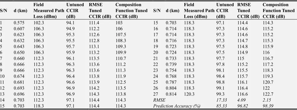
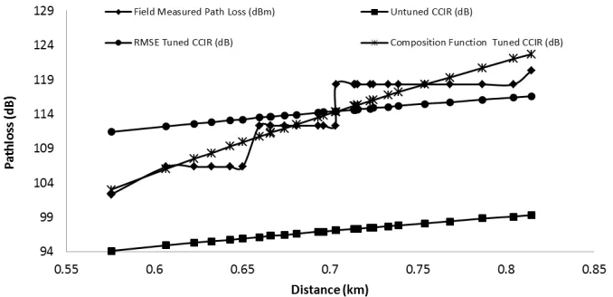
Table 2 and figure 1 show the field measure pathloss and the pathloss predicted by the untuned CCIR model, the pathloss
predicted by the RMSE tuned CCIR model and the pathloss predicted by the composition function tuned CCIR model tuned CCIR model. Also, the table shows that the untuned CCIR model has RMSE of 17.33 dB and prediction accuracy of 85.33%. On the other hand, the pathloss predicted by the RMSE tuned CCIR model has RMSE of 4.09dB and prediction accuracy of 96.82%.and the pathloss predicted by the composition function tuned CCIR model has RME of 2.15 dB and prediction accuracy of 98.39%. Given that RMSE = 17.33 for the then;
PL456789:7;= *+ ) + <=> = PLCDBCDEF • + 17.33 (16)
The composition function is obtained as;
() = K1 ( *+ ) ) +K2
= 2.797895044 ( *+ ) ) + 254.35526 (17)
Then,
PL A BCDEF= *+ ) + ()
= *+ ) + 2.797895044 ( *+ )) + 254.35526 (18)
Table 1. The Field Measured Distance, Received Signal Strength (RSS) and Field Measured Path Loss (PLm).
S/N Distance (km)
Received Signal Strength (dB)
Field Measured Path Loss
(dBm) S/N Distance (km)
Received Signal Strength (dB)
Field Measured Path Loss (dBm)
1 0.5754 -77 102.3 15 0.703179 -93 118.3
2 0.6066 -81 106.3 16 0.71352 -93 118.3
3 0.6227 -81 106.3 17 0.714339 -93 118.3
4 0.6325 -81 106.3 18 0.715505 -93 118.3
5 0.6432 -81 106.3 19 0.722838 -93 118.3
6 0.6503 -81 106.3 20 0.724317 -93 118.3
7 0.6596 -87 112.3 21 0.73273 -93 118.3
8 0.6658 -87 112.3 22 0.738797 -93 118.3
9 0.6660 -87 112.3 23 0.753736 -93 118.3
10 0.6741 -87 112.3 24 0.76781 -93 118.3
11 0.6812 -87 112.3 25 0.786526 -93 118.3
12 0.6931 -87 112.3 26 0.804117 -93 118.3
13 0.6964 -87 112.3 27 0.814393 -95 120.3
14 0.7029 -87 112.3
Table 2. The field measure pathloss and the pathloss predicted by the untuned and the tuned CCIR models.
S/N d (km) Field
Measured Path Loss (dBm)
Untuned CCIR (dB)
RMSE Tuned CCIR (dB)
Composition Function Tuned CCIR (dB)
S/N d (km) Field
Measured Path Loss (dBm)
Untuned CCIR (dB)
RMSE Tuned CCIR (dB)
Composition Function Tuned CCIR (dB) 1 0.575 102.3 94.1 111.4 103 15 0.703 118.3 97.1 114.4 114.3 2 0.607 106.3 94.9 112.2 106 16 0.714 118.3 97.3 114.6 115.2 3 0.623 106.3 95.3 112.6 107.5 17 0.714 118.3 97.3 114.6 115.2 4 0.632 106.3 95.5 112.8 108.3 18 0.716 118.3 97.3 114.7 115.3 5 0.643 106.3 95.7 113.1 109.3 19 0.723 118.3 97.5 114.8 115.9 6 0.650 106.3 95.9 113.2 109.9 20 0.724 118.3 97.5 114.9 116 7 0.660 112.3 96.1 113.5 110.7 21 0.733 118.3 97.7 115 116.7 8 0.666 112.3 96.3 113.6 111.2 22 0.739 118.3 97.8 115.2 117.2 9 0.666 112.3 96.3 113.6 111.3 23 0.754 118.3 98.1 115.5 118.3 10 0.674 112.3 96.4 113.8 111.9 24 0.768 118.3 98.4 115.7 119.3 11 0.681 112.3 96.6 113.9 112.5 25 0.787 118.3 98.8 116.1 120.7 12 0.693 112.3 96.9 114.2 113.5 26 0.804 118.3 99.1 116.4 122 13 0.696 112.3 96.9 114.3 113.8 27 0.814 120.3 99.3 116.6 122.7
14 0.703 112.3 97.1 114.4 114.3 RMSE 17.33 4.09 2.15
Figure 1. The field measure pathloss and the pathloss predicted by the untuned and the tuned CCIR models.
4. Conclusion
In this paper, comparative study of two CCIR pathloss model tuning approaches is presented. Both methods are least square methods. The first model tuning approach is implemented by the addition or subtraction of the root mean square error (RMSE) based on whether the sum of errors is positive or negative. The second method is implemented by adding a composition function of the residue to the original CCIR model pathloss prediction. The study is based on field measurement carried out in a suburban area for a GSM network in the 1800 MHz frequency band. The results show that the composition function approach has better pathloss prediction performance with smaller RMSE and higher prediction accuracy than the RMSE-based approach.
References
[1] Cheng, E. M., Abbas, Z., AbdulMalek, M., Lee, K. Y., You, K. Y., Khor, S. F., & Afendi, M. (2016). Geometrical Optics Based Path Loss Model for Furnished Indoor Environment. Applied Computational Electromagnetics Society Journal, 31(9), 1125-1134.
[2] Popoola, S. I., & Oseni, O. F. (2014). Empirical Path Loss Models for GSM Network Deployment in Makurdi, Nigeria. International Refereed Journal of Engineering and Science (IRJES), 3(6), 85-94.
[3] Chrysikos, T., & Kotsopoulos, S. (2013, March). Site-specific Validation of Path Loss Models and Large-scale Fading Characterization for a Complex Urban Propagation Topology at 2.4 GHz. In Proceedings of the International MultiConference of Engineers and Computer Scientists (Vol. 2, pp. 2078-0958).
[4] Abdul Aziz, O., & Rahman, T. A. (2014). Investigation of Path Loss Prediction in Different Multi-Floor Stairwells at 900 MHz and 800 MHz. Progress In Electromagnetics Research M, 39, 27-39.
[5] Chebil, J., Lawas, A. K., & Islam, M. D. (2013). Comparison between measured and predicted path loss for mobile communication in Malaysia. World Applied Sciences Journal, 21, 123-128.
[6] Rakesh, N., & Srivatsa, S. K. (2013). A study on path loss analysis for gsm Mobile networks for urban, rural and Suburban regions of Karnataka state. International Journal of Distributed and Parallel Systems, 4(1), 53.
[7] Faruk, N., Ayeni, A., & Adediran, Y. A. (2013). On the study of empirical path loss models for accurate prediction of TV signal for secondary users. Progress In Electromagnetics Research B, 49, 155-176.
[8] Okorogu, V. N., Onyishi, D. U., Nwalozie, G. C., & Onoh, G. N. (2013). Empirical Characterization of Propagation Path Loss and Performance Evaluation for Co-Site Urban Environment. International Journal of Computer Applications, 70(10).
[9] Erceg, V., Greenstein, L. J., Tjandra, S. Y., Parkoff, S. R., Gupta, A., Kulic, B.,... & Bianchi, R. (1999). An empirically based path loss model for wireless channels in suburban environments. IEEE Journal on selected areas in communications, 17(7), 1205-1211.
[10] Abhayawardhana, V. S., Wassell, I. J., Crosby, D., Sellars, M. P., & Brown, M. G. (2005, May). Comparison of empirical propagation path loss models for fixed wireless access systems. In 2005 IEEE 61st Vehicular Technology Conference (Vol. 1, pp. 73-77). IEEE.
[11] Awada, A., Wegmann, B., Viering, I., & Klein, A. (2011). Optimizing the radio network parameters of the long term evolution system using Taguchi's method. IEEE Transactions on vehicular technology, 60(8), 3825-3839.
[12] Phillips, C., Sicker, D., & Grunwald, D. (2013). A survey of wireless path loss prediction and coverage mapping methods. IEEE Communications Surveys & Tutorials, 15(1), 255-270.
[13] Chebil, J., Lawas, A. K., & Islam, M. D. (2013). Comparison between measured and predicted path loss for mobile communication in Malaysia. World Applied Sciences Journal, 21, 123-128.
[14] Sharma, P. K., & Singh, R. K. (2011). Comparative Study of Path loss Models depends on Various Parameters. IJEST, 3(6). [15] Mousa, A., Dama, Y., Najjar, M., & Alsayeh, B. (2012).
Optimizing Outdoor Propagation Model based on Measurements for Multiple RF Cell. International Journal of Computer Applications, 60(5).
[17] Bhuvaneshwari, A., Hemalatha, R., & Satyasavithri, T. (2013, October). Statistical tuning of the best suited prediction model for measurements made in Hyderabad city of Southern India. In Proceedings of the world congress on engineering and computer science (Vol. 2, pp. 23-25).
[18] Kale, S. S., & Jadhav, A. N. (2013). Performance analysis of empirical propagation models for WiMAX in urban environment. OSR J. Electron. Commun. Engin. (IOSR-JECE). [19] Al Mahmud, M. R. (2009). Analysis and planning microwave link to established efficient wireless communications (Doctoral dissertation, Blekinge Institute of Technology).
[20] Walter D., (2006) R.F. Path-loss and Transmission distance calculations. Axon, LLC, Technical memorandum 2006.
[21] Negi, A. (2006). Analysis of Relay-based Cellular Systems. [22] Muhammad, J. (2007). Artificial neural networks for location
estimation and co-cannel interference suppression in cellular networks.
[23] Ajose, S. O., and Imoize, A. L. (2013). Propagation measurements and modelling at 1800 MHz in Lagos Nigeria. International Journal of Wireless and Mobile Computing, 6(2), 165-174.
[24] Seybold, J.S. (2005) Introduction to RF Propagation, John Wiley and Sons Inc., New Jersey.