http://www.sciencepublishinggroup.com/j/ajmie doi: 10.11648/j.ajmie.20170204.11
Modeling and Optimization of Shell and Tube Heat
Exchanger in Treatment Unit of South Pars Fifth Refinery
by Fluent Software
Kazem Moaveni
*, Mehran Zarkesh
Department of Mechanic, Dashtestan Branch, Islamic Azad University, Borazjan, Iran
Email address:
[email protected] (K. Moaveni) *
Corresponding author
To cite this article:
Kazem Moaveni, Mehran Zarkesh. Modeling and Optimization of Shell and Tube Heat Exchanger in Treatment Unit of South Pars Fifth Refinery by Fluent Software. American Journal of Mechanical and Industrial Engineering. Vol. 2, No. 4, 2017, pp. 150-161.
doi: 10.11648/j.ajmie.20170204.11
Received: April 11, 2017; Accepted: April 21, 2017; Published: July 4, 2017
Abstract:
In this thesis, the numerical solution of navier stockes equations and turbulent equations have also been investigated in fluent software, to investigate baffle type change from cut off to helical in shell and tube heat exchanger. RNG K-ε turbulence model was used to perturbations modelling. The main objective of baffle changing in thesis is increasing propane temperature in pipes outlet. 4 heat exchanger type with different helical angles (35, 40, 45 and 50) compared with simple baffle type. Studies indicate that heat exchanger with helical angle of 50°, maximum outlet temperature of propane will result and have the maximum heat transfer rate in shell. Exchangers with helical angle of 40 degrees have the highest ratio h / ∆p, which reflects the heat transfer rate to pressure drop ratio.Keywords: Optimization, Shell and Tube Heat Exchanger, Treatment Unit, Fluent Software
1. Introduction
Equipments used in the heat transfer, defined, according to the operation in the process of doing. heat exchanger, heat between two streams of the process to recovery. steam and cold water are used as ancillary services but such as streams can recover them in the process, not studied.
Heaters for heating of fluids used in the process and often from steam water as the heating fluids is used. however in oil refineries, from hot oil is used in the current cycle for heating and for the cooling of fluids, the dispenser is used and cold water acts as a cooling intermediate matter.
Condenser is kind of cooling but the purpose of using it is to take of the fluid sensible heat.
The purpose of the use of the reboiler, is the necessary heat supply in distillation process as latent heat.
In this study, a shell and tube heat exchanger that used the two fluids of water steam in the shell and propane in the tube, the numerical analysis are considered.
2. Governing Equations
In the chapter, is described, equations and models used in the numerical solution of flow in the heat exchangers. these equation are include, continuity equation, momentum, energy and turbulence equations that to continue with the introduction of them.
2.1. Fluid Flow Relations
In general, Governing equations of viscous flows, are navier-stokes and continuity equations.
When the flow is turbulent, transition move of the fluid particles, identifies non- permanent of flow. so, for the numerical solution of equations, must size of time step in calculation, be considered much smaller of time scales of turbulence. it is also necessary, numerical calculation to be performed in the network that dimensions each of its components, is much smaller than the length scale of turbulence. (Anderson 1998).
usually, the average time of turbulent flows, will be examined. for this purpose, instead of navier – stokes equations is used time-averaged equations. these equations by replacing the relations = + و = + in the navier – stokes equations and after applying the operator of time-averaged obtained. in this relations are و , respectively, the average time of collective velocities and pressure and are وP , secondary speeds or incident of particles and pressure accidental changes.
Unlike conventional definition, for turbulent flow properties where each property of flow is distinct into two part, stream of the average amount of time and the amount of fluctuation.
For compressible flow by defining the average variables of mass weight as:
= (1)
Instead of the time average amount of turbulent flow properties from gathering of average variables of mass and swinging components are obtained that unlike time -average mode, time components are not zero.
= + (2) As such, time-average operator is defined as:
=∆ ∆ (3)
It is noteworthy that average variables of mass weight used only for velocities and temperature components and other quantities such as pressure and density calculated as before.
By replacing the components of turbulent flow (result from the mass average variables) flow equations can be obtained as follows:
Continuity equation:
+ ̅ ! = 0 (4)
momentum equation:
# ̅ $ % + # ̅ $ $ % = − '
(+ )+ −* *! (6)
energy equation:
̅,! + - ̅ $ , + *, − . /0 = − '+ 1)+ + )* *! (6)
That:
)+ = 2 3-* 4+5+ 4+(60 −789 4+::; + 2 3- 45<<+ 46<<(0 −789 4:
<<
:; (7)
Problems solution related to viscous flows by navier-stokes equations of simplification, accuracy is not high. during that there is interaction between viscous and non-viscous areas and flow separation, it is necessary for solution of navier-stokes full equations that this method is time-consuming and costly. (Anderson 1998).
Usually numerical methods for solving navier-stokes equations, is such as solution methods of Euler equations.
If t, the time display and were ρ, p و T, respectively represent the density, pressure and temperature, complimentary U, V, W as velocities in Cartesian coordinates (X,Y,Z), navier-stokes equations of 3D (three-dimensional) in curvilinear coordinates are defined as follows:
= >? + =@ A? − AC! + =B D E? − EB! + =F G? − GC! = 0 B (8)
>? = H I J K L M N O P (9)
A? = ℎ
H I J
R R + S T RK + SUT
RL + SVT
R#M + T% N O P
(10)
E? = ℎ
H I
J K + W+ W T
UT
L + WVT
#M + T% N O P
(11)
G? = ℎ
H I J
X X + Y T XK + YUT
XL + YZT
X#M + T% N O P
(12)
That Q is the conservative variable vector and G?, E?, A are displacement fluids vector and ACB, EB,GC Bare viscous fluids vector and also, e introduced the total energy. (Anderson 1998).
The contract velocities components U, V, W, as defined below:
R = S + SUK + SVL (13)
= W + WUK + WVL (14)
X = Y + YUK + YVL (15)
The equation of state is used for the complete system of equation, the compressible flow:
That \ Is the ratio of specific heat coefficient and also, h is reversed of the transfer Jacobins:
ℎ = `ab@@ abDD abFF
c@ cD cF`
(17)
Viscous fluids vectors are include:
AC = ℎdS AB B+ SUEB+ SVGBe (18)
EB= ℎdW AB+ WUEB+ WVGBe (19)
GB
C = ℎdY AB+ YUEB+ YVGBe (20) In Cartesian coordinates:
AB =
f g g g
h )0 ) U
) V
) + K) U+ L) V− .= ijk
k k l
(21)
EB=
f g g g
h )0U )UU
)UV
)U + K)UU+ L)UV− .=Uij
k k k l
(22)
GB =
f g g g
h )0V )VU
)VV
)V + K)VU+ L)VV− .=Vijk
k k l
(23)
) = 22= −782 = + =UK + =VL! (24)
)UU= 22=UK −782 = + =UK + =VL! (25)
)VV= 22=VL −782 = + =UK + =VL! (26)
) U= )U = 2 =U + = K! (27)
) V= )V = 2#=V + = L% (28)
)UV = )VU= 2 =VK + =UL! (29) Correlation coefficient of viscosity #2% and heat transfer coefficient (k) is defined as:
. =UnU oqrps (30)
Prandtl number (pr), is laminar flow.
By replacing time-averaged quantities total and swinging instead if physical quantities in navier-stokes equations, appear new unknowns in the equations. for complete the system of equations need to add new equation to model of additional phrases. additional introduced new relationships for complete the system of equations called turbulence models. (Anderson 1998).
2.2. Turbulent Flow Models
Turbulent flow models can be classified as follows: (Wilcox 1994)
1) Algebraic models of turbulent viscosity (Zero-equation models)
2) Differential models of turbulent viscosity (the single-equation and two single-equation)
3) Reynolds stress models (Differential and algebraic turbulence models)
4) large eddy simulation of turbulence
5) direct simulation of turbulence( without the use of turbulence models)
Zero-equation models, only the relationships and algebraic equations to describe the relationship between μ and the calculated properties and or measurable used. A equation models, in this between uses from a transport equation of additional PDE. Two-equation models are included two additional PDE.
In the categories of first and second used Boussinesq theory. The means that turbulence tensions calculate according to the stokes viscosity law and flows like to laminar flows.
− * = 2 - 45+ 46(0 (31)
Where μ is turbulence viscosity.
In the third category, directly, obtained turbulence tensions that are from number of transfer equations or differential or algebraic.
In the fourth category, to a certain size of the vortices are examined without of model and for they to solve navier-stokes equations in non-permanent state but the model small vortices.
In the fifth category, turbulent flow are examined without modeling and by solving the navier-stokes equations of non-permanent with in view of the very small distance of time and place turbulence flow is studied.
The last two methods requires the use of very fast computers and generally limited to simple mode and low Reynolds number. because is used in research from two category, so we just preferred to these models.
2.2.1. Single-Equation Model: Spalart-Allmaras
Model Spalart-Allmaras is model of one simple equation that solve a model equation of transfer for get 2 .
Model Spalart-Allmaras, effective model for low Reynolds number is considered, the effective use of this model, is limited to affected areas by the viscosity in inside of the boundary layer and similar areas.
2.2.2. Two-Equation Model
i. Model k-ε
Model k-ε, is the most popular of two-equation model. because it is easy to understand and use it in the program is simple. in models k-ε Eddy-Viscosity, the turbulent square by two variables can be expressed. (Wilcox 1994)
a. The kinetic energy of turbulent (k)
b.Slimy dissolution rate of the kinetic energy of turbulent flow(ε)
. =7 (32)
u = ops ,* ,* (33)
Can by help of dimensional analysis showed that turbulent viscosity (2 % can be linked to the large Eddy scale length of turbulent flow.
2 ∝ w9w (34) Where in w and 9w, are respectively, the speed and length of scale in the biggest Eddy on field of the turbulent flow. in addition, it can be shown that:
w∝ √. (35)
9w ∝ yz
{
| (36)
As a result:
2 = }p z
~
| (37)
Where in }p, is an experimental coefficient that its value is usually considered equal to 0.9. in the standard model k-ε, k and ε, obtained by semi- experimental equations below:
# ̅.% + ̅ *.! = 3o2 +€p•:s z; + G − u − 2 u•7 (38)
# ̅u% + ̅ *u! = 3o2 +€p‚•s |; + } |zG − }7 |
~
z (39)
Where in } and }7 have been experimental coefficients and ƒz وƒ| are respectively, prandtl numbers and turbulent Schmidt.
Terms } |zG „… }7 |z~, respectively are, represent of the processes of shear production ε and viscose filament processes ε. in the above equations,buoyancy effects is not considered.
Term G, is represents of production rate of the turbulent kinetic energy, due to interaction, between the average flow and turbulent flow field and for this purpose, the called shear production term. according to:
G = − 4( (40)
according to the hypothesis Boussinesq:
−ρ *= 2 3 4( + 4(−879 4::; −78 .9 (41)
That 2 is turbulent viscosity coefficient and used for
Reynolds stresses.
G = 32 - 4(+ 4 (−
7 89
4: :0 −
7 89 .;
4( (42)
Also, • is much of turbulent flow, is obtained the following equation:
• = ‡7zˆ~ (43)
That a, is the speed of sound.
Note that term 2 u•7 for compressible flow entered to the equation.
ii. ModelRNG k-ε
Yakhut and his colleagues have presented new model of k-ε that specifications and its function properties in compared to the standard model is optimized. the general form of the equation RNG k-ε, are as follows: (Anderson 1998)
# ̅.% + ̅ *.! = 3o2 +€p•:s z; + G − u − 2 u•7 (44)
# ̅u% + ̅ *u! = 3o2 +€p‚•s |; + } z|G − }7 |
~
z −
‰ŠD{o n‹‹s
ŒD{ | ~
z (45)
Parameter W, is represents of the turbulent characteristic time ratio, to flow field characteristic time. so, this model has determined, effects of Off-Equilibrium.
η= •.
u XℎMŽM • = ‡2• • = •2 ,G
• =7- 4(+ 4(0 (46)
It can be shown that η is function of the ratio •‘’‘rˆ “’ “ z
” •• 'ˆ “’ “ z and it can be stated as follows:
η= ‡}pn •| (47)
Yakhut and his colleagues, proposed the following coefficients for this model:
Table 1. The main coefficients of model RNG for isothermal process.
˜™ ˜š ›œ ›• ›ž Ÿ ¡
0.7179 0.7179 1.42 1.68 0.085 4.38 0.015
iii. k-ωModelWilcox
Basic mode of models k-ω from turbulence frequency ω, instead of rate of slimy collapse ε, used for determine of turbulence. (Wilcox 1998)
In model Wilcox k-ω, the relationship between the length and speed turbulence scale, the 9 and with kand ωshown by the following equation:
9 ∝√z¢ (48)
∝ √. (49) As can be seen, changes in the basic relationships and scales length and …. Can not be seen. the turbulence frequency can be set by phrase u = £. to terms kand ωand turbulent viscosity isobtained by the following equation:
2 = }p ¢z (50)
Transport equations for k, ω in model Wilcox, for compressible flow, are:
# ̅.% + ̅ *.! = 3o2 +€p:•s z; + G − —∗ Œ∗.£ (51)
# ̅£% + ̅ *£! = 3o2 +€p¥•s ¢; + ¦¢zG − —Œ£7 (52)
according to coefficient ¦:
¦ =§¨
§∗ © ª « ¬-•~.«¯
¬-• ~.«¯°
(53)
that ¦∗ are:
¦∗= ¦ ±∗ ©
. ²~ { ¬-•³
¬-• ³ °
(54)
That:
´M =p¢z,¦±= 0.52 (55)
In the case that is Reynolds for high flow, can be written:
¦∗= ¦ ±∗ = 1
Also, for Œ∗can be written:
Œ∗= ¶
1 ·z ≤ 0 ¹º– »:~
¼–– »:~ ·z> 0
(56)
Where in:
·z =¢{ z ¢ (57)
For—∗ we have:
—∗= —∗#1 + 1.5 E#• %% (58) Where E#• %, is the compressibility function
E#• % = ¾•7− 0.0625 • > 0.25 0 • ≤ 0.25 (59)
And also:
—∗= 0.09 Áª¯Â o¬-•Ã s Â
o¬-•Ã sÂÄ (60) also, for— and Œwe have:
— = 0.072 ^1 − 1.5 ∗ Œ(∗
–.–Æ7∗ E#• %_ (61) Œ = Æ–»º–»¥¥ (62) that ·¢ are:
·¢ = ÇÈ#–.–Ê¢%(È:É:({Ç (63)
That for • andΩ we have:
• =7- 4(+ 4
(0 (64)
Ω =7- 4(− 4
(0 (65)
Model wilcox k-ω in compared to standard model k-ε in some processes, including speed reduce and separation is due of adverse pressure gradient, works best. models k-ε, since that are high Reynolds models category (this means that in areas with high Reynolds number can provided good results), for solve the equations, in areas near wall, encountered with many problems. but model Wilcox k-ω, can used for predict of changes in the turbulent variables until the edge of the solid walls.
iv. k-ωShear Stress Transport Model
Shear stress transport model k- £ is very similar to the standard model k- £ but also, includes the following improvements:
a. Model k- £ and model k-u, both in a mixing function, multiplied and two model added with together.
b.Shear stresses transport model has a Damped Cross Diffusion Derivative in equation ω.
c. The definition of turbulence viscosity the change is located. in order to account for the effects of the main shear stresses transferring for turbulent flow.
£ has changed.
These properties is the cause that this model for a wide range of currents, like flows with adverse pressure gradient,
high section and the passing shock wave, compared to model k- £, is much more accurate and safer.
this relationship of model is as follows:
# ̅.% + ̅ *.! = 3o2 +€p:•s z; + G?z− —∗.£ (66)
# ̅£% ̅ *£! 3o2 €p¥•s ¢; G¢& —£7 Ì¢ (67)
In this relationship G?z وG¢ وÌ¢ as defined follows:
G?z ÍÎ…#G, 10 —∗.£% (68)
G¢ ϧ•G (69)
Ì¢ 2#1 & E % ƒ¢~¢ z ¢ (70)
In this model, ¦± in equation (53) is obtained from the following equation:
¦± E ¦±ª #1 & E %¦±~ (71)
iQ„ : Ñ Ò Ó Ò Ô¦±
ª
Œ(ª Œ¨∗ &
–.¼~
€¥ªyŒ¨∗ ¦±~
Œ(~ Œ¨∗ & –.¼
~
€¥~yŒ¨∗
(72)
And K is the kinematic viscosity turbulence:
2 ¢ Õˆ oz ª
Ö∗,Ùª¥×Ø~s,„ 0.31
(73)
E7 tanh#„Žß77% , „Žß7 max ^–.–Ê¢U7√z ,â––B¢U~_ (74)
E tanh#„Žß¼%, „Žß min #max ^ √z
–.–Ê¢U, â––B ¢U~_ ,€ ¼ z
¥~”¥äU~% (75)
Ì¢ Í„a 32 €
¥~¢
z ¢, 10n –;
(76)
And also, Ω is the absolute value of rotation.
In near the walls that model k_ £ is more valid, we have:
ƒzª 1.176,ƒZª 2,— 0.075,—±∗ 0.09,¦ âÊ ƒz~ 1,ƒZ~ 1.168,—7 0.0828
—∗ 0.09,¦ 0.872 Also have:
u —∗£. (77)
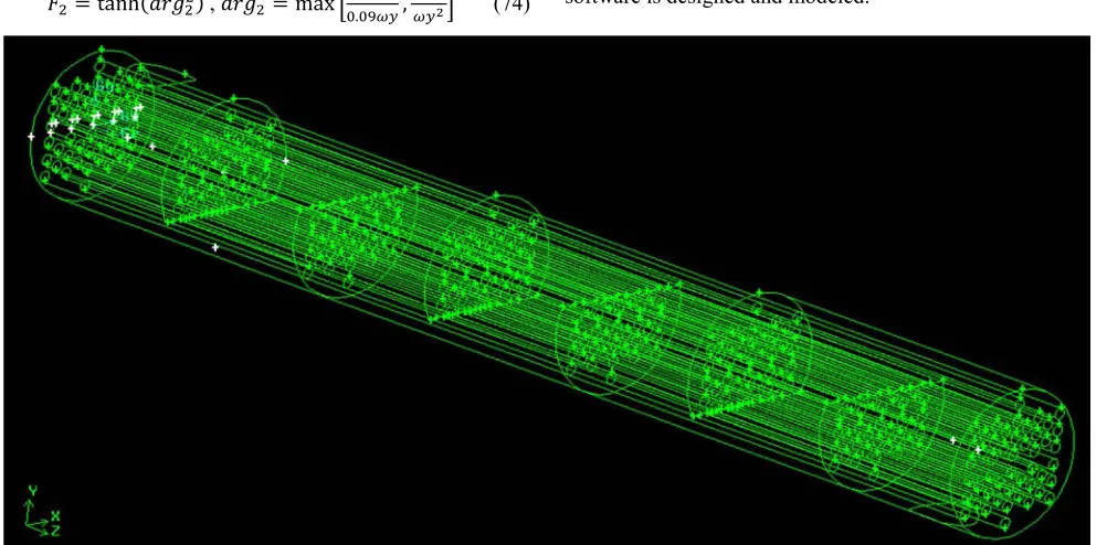
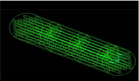
3. Geometrical Production of Exchanger
For geometrical examined in this study is the use of gambit software. figure below shows a view of the shell and tube exchangers with a simple transvers baffle that in this the software is designed and modeled.
Figure 2. A view of the spiral baffle geometry in gambit.
4. Generats the Computational
Grid
Computational network is produced in gambit software. due to geometry of volumes produced, during the design of exchanger are complex, production of organized network in the computational domain, is working very hard. so, in all previous research, from network of computing without
organization, is used for the numerical solution of exchanger. on this basis, in this study, is used from network of without organization with Tetrahedral cells in three dimension and Triangular cells in two dimension.
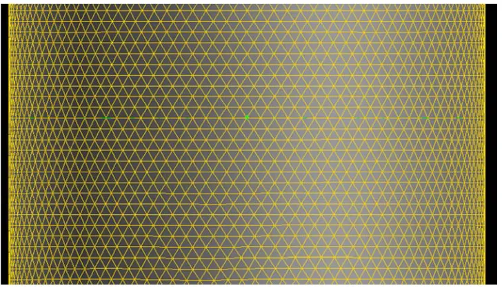
Figure 4 show view of the production network in the exchanger input.
Figure 4. View of the production network in the exchanger input.
Figure 5 also shows a view of the network on the outer body of shell.
Figure 5. A view of the shell outer body network.
5. Validation and Network Study
For validation and network study, 4 network with numbers of computational cells 875000, 2000000, 3500000, 13000000 were compare and investigated. according to the results of this exchanger in the industry,, is propane input with flowrate 80 cubic meters per hour and temperature 35.5°C. for
entering water steam of the shell, is 1628 kg/h for input flowrate and is 161.6 C for input, propane outlet temperature reached about 65°C.
From this information is used for check of the accuracy of numerical solutions on any network.
Figure 6. Propane outlet temperature changes depending on the change in the number of computational cells.
Also, in figure 7 it has been shown, error of output temperature with numerical solution from actual data
Figure 7. Error of the numerical solution of different networks.
It can be seen that error of solution in the networks in after 3500000, is less than 10% and is acceptable.
In figure 8 and 9 also, like previous charts, for pressure drop in shell of networks have been checked that it can be seen, network 3500000 in compared with other networks, the
accuracy is acceptable and also, in compared with network 13000000 cells, has faster convergence.
Figure 8. The pressure drop in the shell in different networks.
Figure 9. Failure to obtain of pressure drop in various network.
6. Numerical Results of Analysis
specifications of exchangers models are investigated and working fluids through of exchanger
According to the research objectives, 5 of model, shell and tube exchanger, has been studied in table 2.
Table 2. Models examined in the study.
MODEL model 1 model 2 model 3 model 4 model 5
Kind of baffle segmental helical helical helical helical
property 7 baffle Angle 35 Angle 40 Angle 45 Angle 50
The first model that is segmental baffle, is tried to be a model, like to industrial exchanger used in south pars gas complex.
It should be noted that is considered, helical angle with the
longitudinal axis of the exchanger.
Also, the working fluids in the shell and tube, has been shown, according to the shell and tube with available information in plot 3
Table 3. Transient fluids characteristics of shell and tube.
Fluid name density (kg/m3) Cp (j/kg.k) Thermal conductivity (w/m.k) viscosity (kg/m.s)
Fluid of passing from shell Water steam 0.5542 2014 0.0261 0.0000134
Fluid of passing from tube propane 1.191 1549 0.0177 0.00000795
Table 4. Profile steal tubes and shells and baffles.
material density (kg/m3) Cp (j/kg.k) Thermal conductivity (w/m.k)
tube A-334 7567.2 445.5 615.456
shell A-516 GR-60 7861.1 447.688 622.64
6.1. Boundary Condition and Initial of Problem
In this problem, is propane input with flowrate 2 cubic meters per hour and temperature 35.5°C. for entering water steam of the shell, is 1628 kg/h for input flowrate and is 161.6°C for input temperature.
6.2. Choose a Suitable Turbulence Model
Considering Fluid flow is turbulent in exchanger, one of the important parts of research, turbulence model is the right choice. for this purpose, three turbulence models RNG K-ε ، K-ω Standard and
SST K-ω was checked for exchanger with segmental baffle and the number of cells by 3500000, that in the three solutions, propane temperature output accuracy and speed convergence of three models, were compared together.
Accuracy of RNG K-ε and SST K-ω models are almost identical, difference is that convergence of model RNG K-ε is faster than SST K-ω model.
Standard K-ω model has less accurate than the other two models. so, model RNG K-ε is used as the model of choice for continuation of analysis.
6.3. Comparing the Model Results
Based on information obtained in the previous section from computational grid with 3500000 cells is used for all of the models.
Also, is used from SIMPLE algorithms and second order discrete in equations solve.
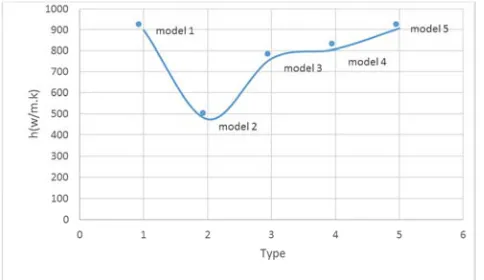
In figure 10 has determined Changes of convection coefficient of the shell inside fluids for baffle different states of shell inside.
Figure 10. Changes of convection coefficient of the shell inside fluids for baffle different states of shell inside.
As you see, model 5 with angle of baffle 50 degree, has the most rate of the heat transfer coefficient.
After model 5, model 1 that is simple segmental baffle,, has the most rate of the heat transfer.
Figure 11 has determine compare the pressure drop of inside the shell for different models of baffle.
Figure 11. Compare the pressure drop of inside the shell for different models of baffle.
From figure 11, it is observed that the most of the pressure drop is related in exchanger with segmental baffle.
For exchangers with helical baffle, by increasing the baffle angle to the longitudinal axis, with the increase in pressure drop.
The parameter that with respect of heat transfer and pressure drop, can more efficient model for us to determine, is ratio of h/∆p. whatever this ratio be the higher, of course is the better.
Figure 12 has determined ratio of h/∆p for different models of baffle.
Figure 12. h/∆p ratio for different models of baffle.
From figure 12, it is clear that model 3 with angle of 40 degree, has the most of ratio h/∆p. model 1 with segmental baffle, has the lowest of ratio that is indicative, lack of suitability this model.
Of course, in a place that temperatures have a major role in the problem and more important goal is to increase heat transfer between two fluids, may is used from the model that has higher heat transfer and it is ignored rate of higher of pressure drop.
Figure 13. Propane outlet temperature.
Figure 14. The temperature distribution inside the exchanger tubes with segmental baffle.
As you can see because opposed to shell and tubes flow, as we get closer to the outlet of tubes, tubes surface temperature has risen.
Figure 15 has showed temperature distribution of the baffles in segmental state.
Figure 15. Temperature distribution of the baffles.
As you can see in segmental simple baffle, pressure drop is high. this is due to the formation of vortices is behind the baffle.
Of course, it would help to increase of heat transfer coefficient because of flow turbulence.
Figure 16 show view of the creation of rest areas and vortex-shaped.
Figure 16. View of the creation of rest areas and vortex-shaped.
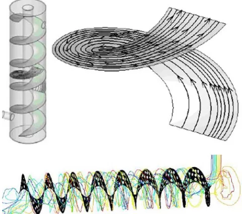
Figure 17 show flow in exchanger with helical baffle that because of the shape of baffle is less vortices and reduced pressure drop in the shell.
7. Offers
Due to the high number of computational cells in such a matter, by taking a large number baffle model and more angles takes many times but the results can be more accurate from flow behavior and obtained heat transfer in exchanger at baffle different angles. also, With more models can by using genetic algorithm, the optimal angle to achieve for higher efficiency of exchanger.
Also, at different Reynolds or in other words, in the flowrates of the fluid inlet deferent, the other results can described for heat transfer and pressure drop in other models according to flow.
8. Conclusion
In this research using numerical solution effect of changing baffle from segmental state to helical state for an industrial exchanger was studied. also, affect of change of helical angle on heat transfer and pressure drop was studied. using network study found that network with 3500000 computational cells is the best option for the numerical solution this exchanger.
Also, with the resulting network, three turbulence models RNG K-ε ، K-ω و SST K-ω for exchanger with segmental baffle that result shown that model RNG K-ε in addition to sufficient accuracy, convergence is good in compare to other models.
With this information, 4 exchangers models with different helical angle were compared with simple exchanger with segmental baffle. survey showed that model 5 with the helical angle of 50 degree, most propane outlet temperature and heat transfer rate that is the highest among other exchangers. but if pressure drop in the shell is also important, it is not optimal. model 3 with an angle of the 40 degree, the highest of the h/dp that is represents rate of heat transfer to pressure drop.
The results of this study can be used in exchangers used in various industries such as oil and gas industries.
Nomenclature
Latin symbols
T fluid temperature (K)
Q conservative variable vector
G? ,E?, A? displacement fluids vector
Ev, Fv, Gv viscous fluids vector
he introduced the total energy
Mt Mach of turbulent flow
cp specific heat (Jkg-1k-1)
∆p overall pressure drop (Pa)
DT logarithmic mean temperature difference (K)
U, V , W velocities in different directions (ms-1) X, Y, Z Cartesian coordinates system (mm) Greek symbols
2 dynamic viscosity (kgm-1s-1)
2 t turbulent dynamic viscosity (kgm-1s-1) νt turbulent dynamic viscosity (kgm-1s-1)
ν kinematic viscosity (m2s-1) ε dissipation rate of turbulent (m2s-3)
density (kg m-3)
a speed of sound
σk Prandtl number of k
σε Prandtl number of ε
Ω rotation absolute value
λ thermal conductivity (Wm-1k-1) Subscripts
In inlet
Out outlet
s shell side
t tube side
References
[1] Holman J. P., 2002. Heat Transfer, 9th Edition, McGraw-Hill. [2] Mills A. F., 1992. Heat transfers, Irwin, USA.
[3] Patankar, S. V., 1980. Numerical Heat Transfer and Fluid Flow”, Hemisphere, New York.
[4] Shah R. K., Sekulic D. P., 2003. Fundamentals of Heat Exchanger Design, John Wiley and Sons, Inc., NJ.
[5] Treybal R. E., 1990. Mass-Transfer Operation, 3rd Edition, Tokyo.
[6] Wilcox D. C., 1994. Turbulence Modeling for CFD. DCW Industries, Inc, California.
[7] Anderson D. A., Tannehill J. C. and Pletcher R. H, 1998.
Computational Fluid Mechanic And Heat Transfer, Mc-Graw-Hill Book Company, Washington D. C, New York And London.
[8] Bahiraei M., Hangi M., Saeedan M., 2015. A novel application for energy efficiency improvement using nanofluid in shell and tube heat exchanger equipped with helical baffles, Energy, Vol. 93, part 2, PP. 2229-2240.
[9] Dizaji H. S., Jafarmadar S., Hashemian M., 2015. The effect of flow, thermodynamic and geometrical characteristics on exergy loss in shell and coiled tube heat exchangers, Energy conversion and management, Vol. 91, PP. 678-684.
[10] Gao B., Bi Q., Nie Z. and Wu J., 2015. Experimental study of effects of baffle helix angle on side performance of shell-and-tube heat exchangers with discontinuous helical baffles. Experimental thermal and fluid Science, Vol. 68, PP. 48-57. [11] Yang J. and Liu W., 2015. Numerical Investigation on a novel
shell-and-tube heat exchanger with plate baffles and experimental validation, Energy conversion and management, Vol 101, PP. 689-696.
[12] Yang J. F., Zeng M., Wang Q. W., 2015. Numerical investigation on combined single shell and tube heat exchanger with two-layer continuous helical baffles, International Journal of Heat and Mass transfer, Vol. 84, PP 103-113.