A Novel Face Recognition Method using
Nearest Line Projection
Huanguo Zhang, Sha Lv, Wei Li and Xun Qu
Department of Electrical Information Engineering, Yibin Vocational & Technical College Yibin, Sichuan 644003, China
Email: [email protected]
Abstract— Face recognition is a popular application of pat-tern recognition methods, and it faces challenging problems including illumination, expression, and pose. The most popular way is to learn the subspaces of the face images so that it could be project to another discriminant space where images of different persons can be separated. In this paper, a nearest line projection algorithm is developed to represent the face images for face recognition. Instead of projecting an image to its nearest image, we try to project it to its nearest line spanned by two different face images. The subspaces are learned so that each face image to its nearest line is minimized. We evaluated the proposed algorithm on some benchmark face image database, and also compared it to some other image projection algorithms. The experiment results showed that the proposed algorithm outperforms other ones.
Index Terms— Face Recognition, Subspace Learning, Near-est Line
I. INTRODUCTION
In recent years, in the face recognition community, the manifold based learning methods [1]–[7] have attracted much attention. Among these methods, locality preserving projection (LPP) [8]–[11] has been the most popular one. It tries to keep the manifold structure of the image in the low-dimensional space by mapping the samples and regularization with a nearest-neighbor graph [12]–[17]. Moreover, this method has been improved into handle the non-linear distribution by the non-linear mapping, and the locally linear embedding (LLE) is proposed [18]– [20]. However, both these methods are unsupervised [21], [22], which ignore the class label information. Although they are useful for dimensionality reduction problem [23], [24], but they are not suitable for supervised classification problem [25], [26]. To solve this problem, some dis-criminant subspace learning methods have been proposed, for example, Linear discriminant analysis (LDA) [27]– [29], etc. These methods learn the transformation matrix by minimizing the intraclass distance and maximizing interclass distance at the same time [30]–[32]. Using this criterion, traditional methods such as LPP and LLE can also be extended to supervised versions. Moreover, using kernel trick, they can also be extended to kernel versions [33]–[35].
A common feature of all these methods is that they are all using with data points as elements, and try to keep
Manuscript received August 10, 2011; revised January 2, 2012; accepted April 16, 2012. c⃝2005 IEEE.
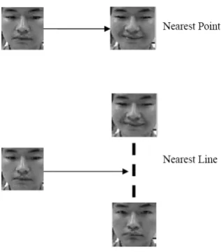
Figure 1. Nearest Point and Nearest Line.
the locality between the data points in the new space. Recently, the nearest linear combination (NLC) method [36] has been proposed. It treat the line between a pair of data points as the basic elements and thus the learning is conducted in a space spanned by the data point lines. To classify a test data point, it is assigned to its nearest line, instead of its nearest point. The difference between the nearest point and nearest point is shown in Figure 1. This classification method has been used and encouraging results are given. But it is only used in classification procedure, and not used in the feature mapping phase.
In this paper, we propose the nearest line project for face image mapping problem. It is different from the traditional data point based subspace learning which try to map the point into a space where it is close to its nearest point. We try to map it so that it is close to its close line. The transitional methods, including LPP and LLE, represent the manifold information by constructing the graph of nearest point. If the number of data points are small, it could not be a good representation of the manifold. To solve this problem, we propose to measure the similarity between a data point to its nearest lines to explorer the manifold better. Moreover, we propose to embed the information between data point and its nearest line in the subspace, not in the classification procedure.
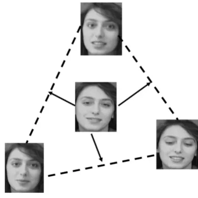
exper-Figure 2. Mapping a face image to its nearest Lines.
iments are conducted to compare the proposed method to other popular projection methods. In section 4, the paper is concluded.
II. NEARESTLINEPROJECTION
We assume that we haventraining data points, denoted as x1,· · · ,xn, and xi ∈ Rd is a d dimensional feature
vector for the i-th data point. Subspace project try to map a data point x to a d′-dimensional space by linear projection
y=W⊤x (1)
andW ∈Rd×d′ is the projection matrix. Usuallyd′≪d
so that the projection could map the data point into low-dimension space.
We hope that after the projection, a data point could be close to its nearest lines. To this end, we need to find
figure 2.
Suppose we have two data points xj andxk inNi, we
project them to the low-dimensional space as yj andyk. The line between them can be given as
Ljk(α) =yjα+yk(1−α) (3)
and the distance betweenyi and this line is computed as the distance betweenyiand its close point at lineLjk(α), as is shown in figure 3. To find the close point, we solve the following problem,
min α
D(α)
=∥yi−Ljk(α)∥22
=∥yi−[yjα+yk(1−α)]
∥2 2
=∥yi−yk−α(yj−yk)∥22
(4)
To solve it, we set the derivative of D(α)with regarding toαto zero,
∂D(α)
∂α =−2
[
(yi−yk)−α(yj−yk)
]⊤
(yj−yk) = 0
α= (yi−yk)
⊤(y
j−yk)
(yj−yk)⊤(yj−yk)
(5) By substituting (5) to D(α), we have the distance of a data point yi to one of its nearest Ljk(α)in (6).
Dist(yi, Ljk;W) =∥yi−yk−α(yj−yk)∥22
=∥yi−yk−
(yi−yk)⊤(yj−yk)
(yj−yk)⊤(yj−yk)
(yj−yk)∥22
=∥W⊤xi−W⊤xk−
(W⊤xi−W⊤xk)⊤(W⊤xj−W⊤xk)
(W⊤xj−W⊤xk)⊤(W⊤xj−W⊤xk)
(W⊤xj−W⊤xk)∥22
=∥W⊤xi−W⊤xk−
(W⊤xi−W⊤xk)⊤(W⊤xj−W⊤xk)
(W⊤xj−W⊤xk)⊤(W⊤xj−W⊤xk)
(W⊤xj−W⊤xk)∥22
=
W⊤
(
xi−xk−
(W⊤xi−W⊤xk)⊤(W⊤xj−W⊤xk)
(W⊤xj−W⊤xk)⊤(W⊤xj−W⊤xk)
(xj−xk)
) 2
2
=T r
[
W⊤
(
xi−xk−
(W⊤xi−W⊤xk)⊤(W⊤xj−W⊤xk)
(W⊤xj−W⊤xk)⊤(W⊤xj−W⊤xk)
(xj−xk)
)
(
xi−xk−
(W⊤xi−W⊤xk)⊤(W⊤xj−W⊤xk)
(W⊤xj−W⊤xk)⊤(W⊤xj−W⊤xk)
(xj−xk)
)⊤
W
]
Figure 3. The distance betweenyiand lineLjk(α).
We hope to learn a projection matrix W so that the distance between each data point to its nearest lines
could be minimized, so we obtain the following objective function in (7),
min W n ∑ i=1 ∑
(j,k)∈Ni
Dist(yi, Ljk;W)
= n ∑
i=1 ∑
(j,k)∈Ni
T r
[
W⊤
(
xi−xk−
(W⊤xi−W⊤xk)⊤(W⊤xj−W⊤xk)
(W⊤xj−W⊤xk)⊤(W⊤xj−W⊤xk)
(xj−xk)
)
(
xi−xk−
(W⊤xi−W⊤xk)⊤(W⊤xj−W⊤xk)
(W⊤xj−W⊤xk)⊤(W⊤xj−W⊤xk)
(xj−xk)
)⊤
W
]
=T r
W⊤ n ∑ i=1 ∑
(j,k)∈Ni (
xi−xk−
(W⊤xi−W⊤xk)⊤(W⊤xj−W⊤xk)
(W⊤xj−W⊤xk)⊤(W⊤xj−W⊤xk)
(xj−xk)
)
(
xi−xk−
(W⊤xi−W⊤xk)⊤(W⊤xj−W⊤xk)
(W⊤xj−W⊤xk)⊤(W⊤xj−W⊤xk)
(xj−xk)
)⊤]
W
}
=T r(
W⊤L(W)W)
(7)
where
L(W) = n ∑ i=1 ∑
(j,k)∈Ni (
xi−xk−
(W⊤xi−W⊤xk)⊤(W⊤xj−W⊤xk)
(W⊤xj−W⊤xk)⊤(W⊤xj−W⊤xk)
(xj−xk)
)
(
xi−xk−
(W⊤xi−W⊤xk)⊤(W⊤xj−W⊤xk)
(W⊤xj−W⊤xk)⊤(W⊤xj−W⊤xk)
(xj−xk)
)]⊤
(8)
Equation (7) is to try to minimize the summarization of the distances between the points and the lines. One other natural way is to try to minimize the summarization of the distances between the points and nearest neighborhood points. The benefit of their solution compared with this alternative lies on that the lines are usually more robust than single points. Mapping to nearest points may lead to noisy results when the points are noisy. However, when nearest lines are considered, even some points are noisy, the mapping could be balanced by other points since lines
are constructed by more than one points.
It is obvious that direct optimization of (7) is difficult, so we use the iterative strategy to learn W. In each iteration, we perform the following two steps:
• UpdateWnew by fixingL(Wold):
Wnew= arg min
W T r (
W⊤L(Wold)W)
(9)
This problem is solved as an eigenvalue problem:
wherew is the eigenvector of L andλis its corre-sponding eigenvalue. We first solve the eigenvectors and eigenvalues, and then rank the eigenvectors according their eigenvalues in descending order, and then pick the first d′ eigenvectors to construct the projection matrixW:
Wnew= [w1,· · ·,wd′] (11)
• Update L(Wnew)by fixingWnew:
L(Wnew) =L(W)|W=Wnew (12)
This procedure is directly and simple.
Actually this algorithm is within the Expectation maxi-mization (EM) algorithms framework [37]–[40]. Updating Wnewby fixingL(Wold)is the maximization step, while
Updating L(Wnew) by fixing Wnew is the expectation
step.
III. EXPERIMENTS
In this section, we perform experiments to compare the proposed algorithms to other methods, on the following several face image databases:
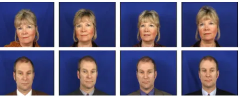
• The ORL Database of Faces [41], [42]: This database is a small database. It only contains 400 images of 40 persons. For each person, there are 10 images in the database. The faces in these images are of frontal view and neutral expression. Moreover, all the images are captured with well-controlled condi-tions, making the recognition quite easy. However, it has been used very popular in the community of face recognition. Example images are shown in 4. • CMU Database of Faces This database is a large
scale database, and there are image of 68 persons. For each person, 170 images are captured. To make the problem difficult, the images are of different lightning, expression and some faces wear glasses. Example images are shown in 5.
• XM2VTS Database of FacesThis database is a face image database of 295 persons, and for each person 12 images are collected. The images are not taken at same time but in different sessions, thus more variety is introduced. significant illumination variety are also included. Example images are shown in 6.
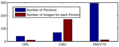
The statistical information of these databases are given in figure 7
We compare our method against the following methods:
LNP NPDA LPP MFA
60 65 70 75 80
Classification Accuracy
Figure 9. Experiment results on CMU database.
LNP NPDA LPP MFA
50 60 70 80
Classification Accuracy
Figure 10. Experiment results on XM2VTS database.
• Marginal Fisher analysis (MFA) [43]–[46]; • Locality preserving projection (LPP) [8]–[11]; • Neighborhood preserving discriminant analysis
(NP-DA) [47]–[50].
We denote the proposed nearest line projection as (LNP). In the experiment, we split the database into two subsets — training set and test set randomly, and the split are performed for 10 times, and the average recognition rates are reported as the results. For classification, we used the nearest neighbor classifier [51]–[54]. The parameters which were using for experiments are as follows: the parameterK (# of the nearest neighborhoods) is set to 6 for the ORL database, 10 for the CMU database, and 6 for the XM2VTS database. EM is stopped for the algorithm for the condition of 100 iterations are reached.
The experiment results on different databases are re-ported in figure 8, 9, and 10. From these figures, we can see that the performance of the NLP is always better than that of the other algorithms. This is an strong evidence that the proposed nearest line based algorithm can outperform the data point based projection methods.
IV. CONCLUSION
Figure 4. Face Images in the ORL Database of Faces.
Figure 5. Face Images in the CMU Database of Faces.
Figure 6. Face Images in the XM2VTS Database of Faces.
problem. The encouraging results showed the advantage of the proposed method. In the future, we will investigate the probability of using the line projection to the matrix factorization problems.
ACKNOWLEDGEMENTS
This study was supported by a grant from the Tianjin Key Laboratory of Cognitive Computing and Application, China.
REFERENCES
[1] S. Wei, C. Ning, and Y. Gong, “Manifold learning based gait feature reduction and recognition,” Journal of Soft-ware, vol. 6, no. 7, pp. 1345–1352, 2011.
[2] L. Zhen, X. Peng, and D. Peng, “Local neighborhood em-bedding for unsupervised nonlinear dimension reduction,”
Journal of Software, vol. 8, no. 2, pp. 410–417, 2013. [3] G. Wang, X. Li, and K. He, “Kernel local fuzzy clustering
margin fisher discriminant method faced on fault diagno-sis,”Journal of Software, vol. 6, no. 10, pp. 1993–2000, 2011.
[4] B. Tang, T. Song, F. Li, and L. Deng, “Fault diagnosis for a wind turbine transmission system based on manifold learning and shannon wavelet support vector machine,”
Renewable Energy, vol. 62, pp. 1–9, 2014.
[5] W.-T. Yao and H.-M. Wu, “Isometric sliced inverse re-gression for nonlinear manifold learning,” Statistics and Computing, vol. 23, no. 5, pp. 563–576, 2013.
“Face image superresolution via locality preserving projec-tion and sparse coding,”Journal of Software, vol. 8, no. 8, pp. 2039–2046, 2013.
[10] J. Qiao and H. Yin, “Optimizing kernel function with appli-cations to kernel principal analysis and locality preserving projection for feature extraction,” Journal of Information Hiding and Multimedia Signal Processing, vol. 4, no. 4, pp. 280–290, 2013.
[11] D. Hu, G. Feng, and Z. Zhou, “Two-dimensional locality preserving projections (2dlpp) with its application to palm-print recognition,”Pattern Recognition, vol. 40, no. 1, pp. 339–342, 2007.
[12] M. Luci´nska and S. Wierzcho´n, “Spectral clustering based on k-nearest neighbor graph,”Lecture Notes in Computer Science (including subseries Lecture Notes in Artificial Intelligence and Lecture Notes in Bioinformatics), vol. 7564 LNCS, pp. 254–265, 2012.
[13] T. Crecelius and R. Schenkel, “Pay-as-you-go maintenance of precomputed nearest neighbors in large graphs,” in
ACM International Conference Proceeding Series, 2012, pp. 952–961.
[14] Z. Liu, C. Wang, and J. Wang, “Aggregate nearest neighbor queries in uncertain graphs,”World Wide Web, pp. 1–28, 2013.
[15] X. Chen, “Clustering based on a near neighbor graph and a grid cell graph,” Journal of Intelligent Information Systems, vol. 40, no. 3, pp. 529–554, 2013.
[16] K. Ozaki, M. Shimbo, M. Komachi, and Y. Matsumoto, “Mutual k-nearest neighbor graph construction in graph-based semi-supervised classification,”Transactions of the Japanese Society for Artificial Intelligence, vol. 28, no. 4, pp. 400–408, 2013.
[17] J. J.-Y. Wang, H. Bensmail, and X. Gao, “Multiple graph regularized nonnegative matrix factorization,” Pat-tern Recognition, vol. 46, no. 10, pp. 2840–2847, 2013. [18] L. Kaiping, C. Binglian, D. Yan, and H. Ying, “A genetic
neural network ensemble prediction model based on local-ly linear embedding for typhoon intensity,” inProceedings of the 2013 IEEE 8th Conference on Industrial Electronics and Applications, ICIEA 2013, 2013, pp. 137–142. [19] X. Liu, D. Tosun, M. Weiner, and N. Schuff, “Locally
linear embedding (lle) for mri based alzheimer’s disease classification,”NeuroImage, vol. 83, pp. 148–157, 2013. [20] H. Li, J. Li, P.-C. Chang, and J. Sun, “Parametric prediction
on default risk of chinese listed tourism companies by using random oversampling, isomap, and locally linear em-beddings on imbalanced samples,”International Journal of Hospitality Management, vol. 35, pp. 141–151, 2013. [21] R. Campello, D. Moulavi, A. Zimek, and J. Sander, “A
framework for semi-supervised and unsupervised optimal extraction of clusters from hierarchies,”Data Mining and Knowledge Discovery, vol. 27, no. 3, pp. 344–371, 2013. [22] L. Li, L. Jin, X. Xu, and E. Song, “Unsupervised color-texture segmentation based on multiscale quaternion gabor filters and splitting strategy,” Signal Processing, vol. 93, no. 9, pp. 2559–2572, 2013.
[23] M. Saeed, K. Javed, and H. Atique Babri, “Machine learning using bernoulli mixture models: Clustering, rule
[26] I. Santos, J. Nieves, P. Bringas, A. Zabala, and J. Sertucha, “Supervised learning classification for dross prediction in ductile iron casting production,” in Proceedings of the 2013 IEEE 8th Conference on Industrial Electronics and Applications, ICIEA 2013, 2013, pp. 1749–1754. [27] G.-F. Lu and W. Zheng, “Complexity-reduced
implementa-tions of complete and null-space-based linear discriminant analysis,”Neural Networks, vol. 46, pp. 165–171, 2013. [28] A. Zollanvari, J. Hua, and E. Dougherty, “Analytical study
of performance of linear discriminant analysis in stochastic settings,” Pattern Recognition, vol. 46, no. 11, pp. 3017– 3029, 2013.
[29] A. Mart´ınez Mar´ın, F. Pe¨na Blanco, C. Avil´es Ram´ırez, L. P´erez Alba, and O. Polvillo Polo, “Selecting the best set of gas chromatography-derived fatty acids to discrimi-nate between two finishing diets using linear discriminant analysis,”Meat Science, vol. 95, no. 2, pp. 173–176, 2013. [30] K. Maliatsos, S. Vassaki, and P. Constantinou, “Interclass and intraclass modulation recognition using the wavelet transform,” inIEEE International Symposium on Personal, Indoor and Mobile Radio Communications, PIMRC, 2007. [31] M. Bala and R. Agrawal, “Decision tree svm frame-work using ratio interclass and intraclass scatters,” in
Proceedings of the 4th Indian International Conference on Artificial Intelligence, IICAI 2009, 2009, pp. 2198–2206. [32] K. Ishida, E. Tushima, Y. Umeno, and S. Satoh, “Intraclass
and interclass reliability of bs-pop,”Rigakuryoho Kagaku, vol. 26, no. 6, pp. 731–737, 2011.
[33] H. Qi and S. Hughes, “Using the kernel trick in com-pressive sensing: Accurate signal recovery from fewer measurements,” inICASSP, IEEE International Conference on Acoustics, Speech and Signal Processing - Proceedings, 2011, pp. 3940–3943.
[34] S. Kung and Y. Luo, “Recursive kernel trick for network segmentation,” International Journal of Robust and Non-linear Control, vol. 21, no. 15, pp. 1807–1822, 2011. [35] T. Ahmed, X. Wei, S. Ahmed, and A.-S. Pathan, “Efficient
and effective automated surveillance agents using kernel tricks,”Simulation, vol. 89, no. 5, pp. 562–577, 2013. [36] S. Z. Li, “Face recognition based on nearest linear
com-binations,” in Proceedings of the IEEE Computer Society Conference on Computer Vision and Pattern Recognition, 1998, pp. 839–844.
[37] T. Covoes and E. Hruschka, “Unsupervised learning of gaussian mixture models: Evolutionary create and elim-inate for expectation maximization algorithm,” in 2013 IEEE Congress on Evolutionary Computation, CEC 2013, 2013, pp. 3206–3213.
[38] Z.-G. Su, P.-H. Wang, Y.-G. Li, and Z.-K. Zhou, “Pa-rameter estimation from interval-valued data using the expectation-maximization algorithm,” Journal of Statisti-cal Computation and Simulation, 2013.
[39] A. Belghith, M. Balasubramanian, C. Bowd, R. Wein-reb, and L. Zangwill, “Glaucoma progression detection using variational expectation maximization algorithm,” in
Proceedings - International Symposium on Biomedical Imaging, 2013, pp. 876–879.
L. Vidal, and J. Benlloch, “Expectation maximization (em) algorithms using polar symmetries for computed tomogra-phy (ct) image reconstruction,”Computers in Biology and Medicine, vol. 43, no. 8, pp. 1053–1061, 2013.
[41] S. Sakthivel, R. Lakshmipathi, and M. Manikandan, “Eval-uation of feature extraction and dimensionality reduction algorithms for face recognition using orl database,” in
Proceedings of the 2009 International Conference on Im-age Processing, Computer Vision, and Pattern Recognition, IPCV 2009, vol. 1, 2009, pp. 367–373.
[42] A. Deleuze, M. Gentili, and G. Vial, “Locoregional anes-thesia in otorhinolaryngology: Nerve blocks of the face [anesthsie locorgionale en orl: Les blocs de la face],” An-nales Francaises d’Anesthesie et de Reanimation, vol. 23, no. 11, pp. 1110–1113, 2004.
[43] Z. Sun, L. Xue, Y. Xu, and H. Wang, “Marginal fisher analysis feature extraction algorithm based on multilayer auto-encoder,”Journal of Information and Computational Science, vol. 9, no. 18, pp. 5897–5906, 2012.
[44] R. Liu, C. Jia, E. Pang, M. Qu, S. Pang, and Z. Yu, “Global and local information based spherical marginal fisher analysis for face recognition,”Journal of Information and Computational Science, vol. 10, no. 4, pp. 1025–1034, 2013.
[45] J. Liu, H. Zheng, S. Pang, C. Wu, C. Jia, and Z. Yu, “Extended marginal fisher analysis based on difference criterion,”Journal of Information and Computational Sci-ence, vol. 10, no. 7, pp. 2051–2058, 2013.
[46] L. Jiang, J. Xuan, and T. Shi, “Feature extraction based on semi-supervised kernel marginal fisher analysis and its application in bearing fault diagnosis,”Mechanical Systems and Signal Processing, 2013.
[47] G. Lu and J. Zuo, “Two-dimensional neighborhood pre-serving discriminant analysis for face recognition,” in Pro-ceedings - 2010 6th International Conference on Natural Computation, ICNC 2010, vol. 7, 2010, pp. 3447–3451. [48] Y.-R. Lin and Q. Wang, “Direct orthogonal neighborhood
preserving discriminant analysis,”Advanced Materials Re-search, vol. 179-180, pp. 1254–1259, 2011.
[49] X. Liang, J. Li, and Y. Lin, “Kernel orthogonal neighbor-hood preserving discriminant analysis,”Advanced Materi-als Research, vol. 339, no. 1, pp. 571–574, 2011. [50] G. Wang and W. Zhang, “Neighborhood preserving fisher
discriminant analysis,” Information Technology Journal, vol. 10, no. 12, pp. 2464–2469, 2011.
[51] A. Lakhotia, A. Walenstein, C. Miles, and A. Singh, “Vilo: A rapid learning nearest-neighbor classifier for malware triage,” Journal in Computer Virology, vol. 9, no. 3, pp. 109–123, 2013.
[52] A. Dhurandhar and A. Dobra, “Probabilistic characteriza-tion of nearest neighbor classifier,” International Journal of Machine Learning and Cybernetics, vol. 4, no. 4, pp. 259–272, 2013.
[53] N. Khoa, D. Viet, and N. Hieu, “Classification of power quality disturbances using wavelet transform and k-nearest neighbor classifier,” inIEEE International Symposium on Industrial Electronics, 2013.
[54] J.-S. Wang, C.-W. Lin, and Y. Yang, “A k-nearest-neighbor classifier with heart rate variability feature-based transfor-mation algorithm for driving stress recognition,” Neuro-computing, vol. 116, pp. 136–143, 2013.
Huanguo Zhang received his B.E. degree in Communication Engineering from Anshan Institute of iron and steel, China in July 2001 and his M.E. degree in Communication and information system from Chongqing University of Posts and Telecommunications, China in June 2005.His current research interest includes communication network, machine learning, and computer vision.
Sha Lvreceived her B.E. degree in Arts from Sichuan Normal University, China in July 2003 and her M.E. degree in Land-scape Architecture from Sichuan Agricultural University, China in June 2009.Her current research interest includes Landscape planning and graphic image processing.
Wei Li received her B.S.degree in Optical information science and technology from Jiangnan University, China in Juny 2004 and her M.E.degree in Electrical and Communication Engineer-ing from Southwest Jiaotong University, China in June 2012. Her current research interest includes Fibre Optical Communi-cation Technology and communiCommuni-cation control.