A Sampling Method Based on Gauss Kernel Learning and the Expanding Research

A Sampling Method Based on Gauss Kernel

Learning and the Expanding Research

Shunzhi Zhu

Department of Computer Science and Technology, Xiamen University of Technology, Xiamen 361024, China Key lab of Spatial Data Mining and Information Sharing, Ministry of Education, Fuzhou University, Fuzhou 350002,

China

Email: [email protected]

Kaibiao Lin, Zhiqiang Zeng, Lizhao Liu

Department of Computer Science and Technology, Xiamen University of Technology, Xiamen 361024, China Email: {kollzok, taoyuan_0302, llz216}@yahoo.com.cn

Wenxing Hong*

Department of Automation,Xiamen University, Xiamen 361005, China [email protected]

Abstract1— In this paper, the expansion of feature points of the linear scale space is transformed into the classification of multi-scale data set within the same scale, which belongs to the classification of scale invariant non-equilibrium .The paper presents a sample approach based on kernel learning to solve classification on imbalance dataset by Support Vector Machine (SVM). The method first preprocesses the data by oversampling the minority class in kernel space, and then the pre-images of the synthetic samples are found based on a distance relation between kernel space and input space. Finally, these pre-images are appended to the original dataset to train a SVM. As a result, the inconsistency which is brought about by processing samples in different spaces is overcome. On the other hand, the sampling strategies of the method not only can decrease imbalanced rate of training dataset, but also can enlarge convex hull of the minority class. Consequently, the problem of the boundary skew can be amended more effectively. Experiments on real dataset indicate that the generalization performance of the result classifier is improved and the algorithm can work well on expanding the feature points stably for a certain scale.

Index Terms—Kernel learning; Convex hull; Kernel space; Pre-image; Scale space

I. INTRODUCTION

Your goal is to simulate the usual appearance of papers in a Journal of the Academy Publisher. We are requesting that you follow these guidelines as closely as possible.

In recent years, the technology of the linear scale space become the hot tool in the areas of computer vision, pattern recognition, image processing, which is more powerful in dealing with feature point detection and

*the corresponding author.

The work is supported by: The national natural science Foundation (61070151); Natural science foundation of fujian province(2010J01353); Open fund from lab of spatial data mining and information sharing of ministry of education of china at university (201001); Open fund from fujian key lab of brain simulation and intelligent system (BLISSOS2010102).

extraction. For instance, the famous LOG operator [1] [2], DOG operator [3] [4], SIFT algorithm [5] and HARRIS - AFFINE algorithm search the feature points [6] all through locating of the cross-scale extreme value. The results of the follow-up identification and processing are depended on the number and stability of feature points. HARRIS points those different types of feature points can expand according to the relationship with the surrounding neighboring points. Mikolajczyk expands the multi-scale characteristic points [7] by utilizing the cross-scale HARRIS operators. However, the number of feature points generating through extended algorithm meeting the basic stability are limited or even reduced. The paper presents a approach to expanding the invariable characteristic point by using the sampling method of Gaussian kernel function cooperating with the SVM algorithm on all levels of linear scale space, which classifying on imbalance dataset by means of kernel function and the condition of fixed scales to achieve the steady expansion of the original feature point set. The number of samples of the non-equilibrium data set is obviously less than other types of sample data sets, and traditional classification approaches, for example, decision tree and neural network are difficult to obtain satisfactory classification results on the non-equilibrium data set.

into two categories: cost –sensitive learning and sampling. The cost –sensitive learning [9] [10] [11] reduces the offset degrees of classification hyperplane by introducing the penalty coefficient to error-classifying positive and negative class samples to improve the generalization performance of the results classifier. Nevertheless, this method needs to modify the classification algorithm, so it is inflexibility. Sampling law without modification of the classification algorithm preprocesses the data to reduce the degree of sample imbalance. The researchers [12] [13] [14] reduce the data sampling imbalances by under-sampling the negative class samples and obtain some achievements. However, the under-sampling ignoring the potential useful negative class samples, and they may reduce the capability of classifier [15]. In contrast with the under-sampling method, the up-sampling reduces the degree of data imbalance by increasing the number of positive class samples, the method receive the better result than the under-sampling due to its avoiding the loss of key samples. Representing for the SMOTE （ Synthetic Minority Over-sampling Technique） _{[16], the} up-sampling constructs the new positive samples by connecting the positive class with their neighbors to increase the number of positive class samples, and arousing widespread interest for its good results. From then on, many improved algorithm are proposed based on the SMOTE, for instance, Akbani introduces the SDC（ SMOTE with Different Costs)[17] combining the SMOTE with Cost-sensitive training. Yang Liu et al present the EnSVM （ Ensemble of SVM ） [18] combining the SMOTE with the Boost. The experiment demonstrates that, these methods have achieved better classification results in non-equilibrium data sets. However, the SMOTE algorithm operating in the input space, but SVM work in kernel space, the best samples constructed in the input space are not necessarily the best in kernel space, in addition, though, the in-sampling of the SMOTE can increase the density of the positive class samples and reduce data imbalances, it can not extend the convex hull formed by the positive class. When the original class of sample distribution is more concentrated, the offset correction of classification hyperplane with the algorithm is more limited, thus affecting the classification performance [19]. In view of this, the paper proposes a novel sampling algorithm, in which, the innovations are list as follows: the new algorithm synthesize new samples in kernel space, consequently, resolve the inconsistent data problem arising from dealing with training samples at different spaces; The sample mode of the new algorithm including the in-sampling and out-sampling, reduces the data imbalance and extend the convex hull formed by the positive class sample simultaneously. So it can correct the Hyperplanes offset problem the more progress and enhance the classification.

II.BACKGROUNDS

The researches of Koenderink (1987) and Lindeberg (1994) indicate that, under variety of reasonable

assumptions, the only possible linear scale space kernel is Gaussian kernel, therefore, in the sense; the Gaussian scale space refers to the scale space.

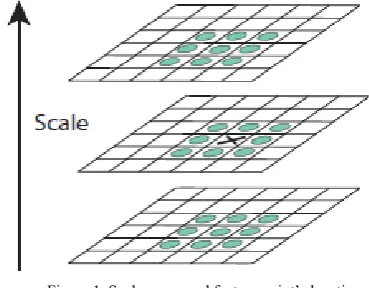
where, L(x,y) satisfies the thermal diffusion equation, and the cross-scale extremum of Gaussian difference function is similar to Laplacian extremum of Gaussian function, which can be used to select the feature points of the linear scale and location of scale-invariant, as shown in figure 1.

Figure 1. Scale space and feature point’s location

，

We can introduce the training process into the scale space especially for the nonlinear scale space named Gradient dependent diffusion:

It belong to the following function in essence:

Or the famous N order diffusion named

As Bart.M said in the first stage, retina to LGN is completely uncommitted and we may not have something else as a linear stage. The RF’s in the LGN show a center-surround structure like this:

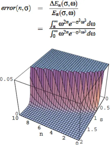
Often not or barely mentioned, there is a massive projection of fiber backwards from primary cortex to LGN.So in the LGN frame the SVM and other similar tools can work in the scale space as it does in the normal space. However, it is widely expanded in the original space and which is known from B. M. ter Haar Romeny we need to take care of the accuracy for example considering the powerspectrum the square of the signal. The aliasing error can be defined as the relative integrated energy of the aliased frequencies over the total energy,as shown in figure 3:

Figure 3. The error of changing calculate space

The essence of training SVM is to solve the optimal classification hyperplane problem, given training samples( , ),x yi i i=1,...,l, where i

,

h

x ∈R y ∈ − _{, so} the optimal classification hyperplane can be transformed into a quadratic optimization problem:

minw b, ,ξ ₁ 1

2

l T

i i w w C ξ

=

+

∑

, (1) Subject toy wi( Tϕ( )xi +b) 1≥ −ξi, ξi ≥0,i=1,...,l

.

Whereξi , i=1,…,l is the relaxation factor, and C>0 is

the penalty coefficient of the mistaken sample, utilizing the Lagrange multiplier method can obtain the dual problem of the mode (1):

min α

1 2

T T

Q e

α α− α

, (2) Subject to0≤αi ≤C i, =1,...,l, 0

T

yα = _.

where e is a vector of 1, αi, i=1,…,l are Lagrange

multipliers, and Q is the symmetric matrix for l×l _,

which is called Hessian matrix.

( , )i j ( ) ( ) T

ij i j i j i j

Q = y y k x x = y yϕ x ϕ x

，k x x( , )i j is the

kernel function, which corresponds to the nonlinear mapping ϕ:Rh F _{, mapping the training samples}

from the input space to a kernel space F, in the nuclear space, the sample is linearly separable. The forms of classification hyperplane of functions from SVM training are follows:

1

( ) sv ( , )

N

i i i

i

f x α y k x x b =

=

∑

. (3) From the geometric point of view, the optimal classification hyperplane obtain by SVM training is perpendicular to the line, which is connected between the nearest points of the two convex hull composed by the positive and negative class samples, and divides it.(As shown in figure 4). Due to the smaller number of the positive class samples, for Non-equilibrium data set, the convex hull are less formed, which led to the classification hyperplane obtained from SVM training shift to the positive class data. Therefore, it is easy to mistake the positive class data into the negative data, thus affecting the classification results.

Figure 4. Optimal classification hyperplane

Ⅲ.SAMPLEINGMETHODBASEDONKERNEL SPACE

The sampling method presented in this section has two differences compared with the SMOTE commonly used at present.

(2) The proposed sampling method not only increases the samples and reduce the data imbalance, but also extend the convex hull formed by the positive class samples. For non-equilibrium data set, due to the small number of positive class samples, the formed convex hull is much smaller in most cases. According to the geometric interpretation of SVM shows, this will led to the classification hyperplane obtained from SVM training shift to the positive class data, thus affecting the classification results. The SMOTE constructs the new samples to increase the number of samples by connecting the two points of the positive class samples. However, the samples synthesized in this method are always within the convex hull, according to the definition of the convex hull, it can not extend the convex hull, even can reduce the convex hull, so it is difficult to correct the offset classification hyperplane effectively. Considering that, the proposed sampling method in this paper can not only synthesize the new samples in the positive class convex hull, but also construct the new positive class samples on the connection between the positive class sample and its negative class sample to extend the positive class convex hull. Consequently, it realizes the correction of offset classification hyperplane.

A. Sampling strategy

Suppose that D { , ,..., }x x1 2 xn

+ ₌

，

1 2

{ n , n ,..., }m

D− = x+ x+ x _， x_i∈Rh_{, i=1,…,m are the}

preprocessing positive and negative class sample sets, the kernel function k( , ) associates with the nonlinear mapping, and the ϕ maps the elements of D+_， D−

from input space into the kernel space F. The algorithm framework of samples synthesized in nuclear space is described as follows:

Input: the positive and negative class sample sets D+

，D−_{, nearest neighbor number k, N represents the ratio}

of the numbers of reconstruct positive class samples and the original sample| D+|

Output: set of the synthetic positive class sample Ds getRandomPoint(S): any element back to the set S getFeatureNeighbors(x, S, k): the return values of k-nearest neighbor of samples x obtained from set S in nuclear space

getRandomNumber(value1,value2): return an arbitrary interval between the values (value1 value2)

getNearestPoint(x,S): return the element in set S which nearest with x

Algorithm:

1) T: = | D+|,Ds:= ∅;

2) if N < 1 then 3)T:=⎢⎣N T× ⎥⎦, N: = 1; 4) end if

5) N: =⎢ ⎥⎣ ⎦N , Z: = D+; 6) for i := 1 to T

7) {xi: = getRandomPoint(Z);

8)Di:= getFeatureNeighbors (xi,(D D ) { }xi

+_∪ − ₋

k); //computing k-nearest neighbors of x in all data sets

9) Di +

:= Di ∩D+

; Di −

=: Di ∩D−

; //obtaining the neighbors of the positive and negative class respectively

10) PositiveNUM: = |Di +

|; NegativeNUM: = |Di −

|; 11) if PositiveNUM <= NegativeNUM then Continue; //the number of negative class neighbors is larger than the number of positive class neighbors, determine the sample is noise and do not synthesize the new samples

12) M+=⎢_⎣N×PositiveNUM k/ ⎥_⎦;M− _=N−M+

; /* synthesizing the new sample between the sample and its positive class neighbor*/

13) for j := 1 to M+

14) {xj: = getRandomPoint (Di+);

15)λij:= getRandomNumber (0, 1);

16)Oij: ( )=ϕ xi + ×λij ( ( )ϕ xj −ϕ( ))xi ; // synthesizing the

new sample in the nuclear space (4) 17)Ds:=Ds∪{ }Oij ;

18) Di+ := Di+ – {xj} ;}

/* synthesizing the new sample between the sample and its negative class neighbor to extend the positive class convex hull */

19) for l := 1 to M−

20) {xl: = getNearestPoint (xi,Di−);

21)λil:= getRandomNumber (0,1/2);

22)Oil: ( )=

ϕ

λ

ϕ

ϕ

the new sample in the nuclear space (5)

23)Ds:=Ds∪{ }Oil ;

24) Di− := Di− – {xl};}

25) Z: = Z – {xi};} 26) Return Ds

The algorithm involves the distance calculation of sample points in the nuclear space, the distance of any two samples ( )ϕ x _{, ( )}ϕ y _{in nuclear space is calculated as} follow:

|| ( )ϕ x −ϕ( ) ||y = k x x( , ) 2 ( , )− k x y +k y y( , ) ₍₆₎ B. Searching the preimage of the synthetic sample

the unknown nonlinear mapping ϕ−1:F→Rh _{, so} searching the accurate preimage uij=ϕ−1( )Oij of the

synthesized samples in the input space is impossible, only the approximate solution can be obtained by some other methods. This article adopts the strategy in literature [20], utilizing the distance relation between the input space and nuclear space to search the preimage zij of synthesized sample in the input space.

The distance relation between the input space and the nuclear space must to be established first before

confirming the preimage. At present, we only establish the distance relation for the isotropic Gaussian kernel function k(x,y)=K(||x-y||) when aiming at the linear scale space. Considering the most widely used of this kernel function in practical application, the algorithm still has prominent practical applicability. In nuclear space, the distance between any element of the original positive class set D+ and the synthetic sample Oij is calculated as follow:

2_{( , ( ))} 2_{( ( ) ( ( ) ( )), ( )) || ( ( ) ( ( ) ( ))) ( ) ||}2

ij i ij j i i ij j i

l l l l l

d O ϕ x =d ϕ x + ×λ ϕ x −ϕ x ϕ x = ϕ x + ×λ ϕ x −ϕ x −ϕ x

(7)

2 2

( , ) 2(l l ij 1) ( , ) 2l i ij ( , ) (l j ij 1) ( , ) 2 (1i i ij ij) ( , )i j ij ( , )j j

k x x λ k x x λ k x x λ k x x λ λ k x x λ k x x

= − − − + − + − +

For Gaussian kernel function, the distance

2_{( ( ), ( ))}

ij

l l

d ϕ u ϕ x _{between the xl and the preimage of Oij in}

the nuclear space and the distance d u xl2( , )ij l between the

xl and the preimage of Oij in the input space maintain the following relationship:

2

_{( ( ), ( )) || ( )}

_{( ) ||}

_{( , ) 2 ( , )}

_{( , )}

ij ij ij ij ij

l l l l l l

d

ϕ

u

ϕ

x

=

ϕ

u

−

ϕ

x

=

k u

u

−

k u

x

+

k x x

2 2 2 2

2 2 exp( ||

−

−

u

−

x

|| /(2

σ

)) 2 2 exp(

= −

−

d

( , ) / (2

u

x

σ

))

_{( , )}

₂

_ln(1

1

_{( ( ), ( )))}

2

ij ij

l l l l

d

u

x

σ

d

ϕ

u

ϕ

x

⇒

= −

−

. (8) For d Ol2( , ( ))ij ϕ xl =dl2( ( ), ( ))ϕ uij ϕ xl , according to the

Esq.(7) and (8), we can obtain d u xl2( , )ij l , which is the

distance between the sample xl and the preimage of Oij in the input space. Generally, the distance between the sample and its neighbor plays an important role in the process of determining the location of sample point, so in the process of solving the uij, we mainly consider the distance between synthetic sample Oij in the nuclear space and its neighbors { ( ), ( ),..., ( )}ϕ x1ij ϕ x2ij ϕ xtij in the input

space (using quadratic to measure). Defining vector as follow:

2 2 2 2 1 2 [ , ,..., ]T

t

d = d d d _{, (9)} Where dl, l=1,…,t is the distance between the preimage of Oij and its neighbor in the input space. The literature [20] adopts the distance constraint between the some unknown coordinate point and other point to confirm the coordinate in the space, the author references

the idea for searching the preimage uij of Oij in the input space.

IV. RESULTSANDANALYSISOFTEST

Overlapping test has been applied here, dividing four parts of each data set, ensure every divided set with the same non-balance rate. In every test, three of them are used as training set and others as testing set. Here the final result is the average. Gauss function is used for all tests, C of LIBSVM and σ of Gauss function is gotten as the optimization by overlapping testing ten times based on a small random data set.

A. Technical norm

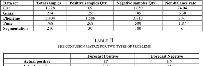
Table 2 is garble matrix, TP-Positive samples Qty, TN-Negative samples Qty, FP-forecast Positive samples Qty, FN-Negative samples Qty.

TABLE I

PAPERS DESCRIPTION OF THE EXPERIMENTAL DATA SET

Data set Total samples Positive samples Qty Negative samples Qty Non-balance rate

Car 1,728 69 1,659 24.04

Glass 214 29 185 6.38

Phoneme 5,404 1,586 3,818 2.41

Pima 768 268 500 1.87

Segmentation 210 30 180 6

TABLE Ⅱ

THE CONFUSION MATRIX FOR TWO TYPES OF PROBLEMS

Forecast Positive Forecast Negetive

Actual positive TP FN

In the application of non-balance data set, dividing result is focused on as [7][9]：

g= acc+⋅acc− ₍₂₀₎

Technical norm of algorithm effective, here：

,

TP acc

TP FN

+₌

+ ,

TN acc

TN FP

−₌

+ ₍₂₁₎

We see:acc+_，acc− acc+₍acc−_{) lower, g smaller} means more errors for divisions of samples with small number. Moreover, the cost is higher of wrong division. B. Result and analysis

Results of test as table 3：

TABLE III

THE G VALUE OF DIFFERENT ALGORITHMS

Data set SVM SMOTE Kernel_SMOTE The Proposed Method

Car 0 0.9884 0.9875 0.9910

Glass 0.8658 0.9236 0.9328 0.9527

Phoneme 0.8276 0.8347 0.8543 0.8556

Pima 0.7119 0.7456 0.7833 0.7820

Segmentation 0.9184 0.9773 0.9865 0.9884

Average 0.5540 0.8939 0.9089 0.9139

In above five data set, SVM gets the smallest g, ours gets the highest g and Kernel_SMOTE get the value of g larger than one by SMOTE. This means consistency issue between atomic space and primary space can be handled by the mentioned algorithm. And, the distributed feature is more similar with ones of primary space. Meanwhile, except Pima data set, g values gained by the mentioned

algorithms are higher than ones by Kernel_SMOTE. This means: if with expanding outward shell generated by positive samples, it will more effective to deal with the issue of hyperplanefaraway. And the classifiergained by the mentioned way is with better feature of generalization.

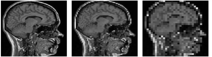
Figure 5. Linear scale space image of CT test image one

Figure 6. Non-linear scale space image of CT test image

Brain CT scanning photo with clear changes has been selected. The space is as showing as Figure 5,6. SIGMA (N) =SIGMA (N-1)*SIAMA (N-1), SIGMA1=0.707. Expanding features of each level in scale space by using mentioned algorithm sampling with SVM algorithm,

because repeating sampling occurs based on LOG operator with better stability. If with the same stability, the mentioned algorithm is with most expanding features in low scale. In high scale, only the qty of expanding features generated by Harris is larger than one by ours.

But there are without two properties: across-scale property and scale fixity by using HARRIS operator. So the mentioned algorithm is advanced in the aspect of stability, translationrotation fixity and sample quantity.

TABLE IV

FEATURE POINT VALUE OF DIFFERENT ALGORITHMS EXTENSION

Scale LOG HARRIS HARRISAFFINE The Proposed Method

SIGMA1 1328 1589 1207 1602

SIGMA2 1109 1018 934 1133

SIGMA3 906 973 870 925

SIGMA4 352 492 348 461

SIGMA5 22 33 19 32

V. SUMMARY

For latest target of expanding characteristic points in scale space, a new algorithm has been mentioned in this paper, which is effective in atomic space for keeping training samples' consistency in different space; Otherwise, increasing qty of positive samples, decreasing negative ones and expanding the outward shell formed by positive ones make more efficient to deal with the faraway of positive hyperplane. Next step, the improvement of this algorithm should be made with more strong suitability in more different assignments.

ACKNOWLEDGMENT

This work is supported by the Natural Science Foundation of Fujian Province（_2010J01353）_{; Open} Fund (201001) Funding from key lab of Spatial Data Mining and Information Sharing, Ministry of Education, Fuzhou University ;Open Fund (BLISSOS2010102) Funding from key lab of of Brain Imitation Intelligent Systems in Xiamen University Fujian Province.

REFERENCES

[1] J. J. Koenderink. The structure of images. Biol. Cybern., 1984, 50:363–370. .

[2] J. J. Koenderink. Design principles for a front-end visual system. In Rolf Eckmiller and Christoph v. d.Malsburg, Neural Computers. Springer-Verlag, 1987, 5:161–168. [3] T. Lindeberg. Scale-space for discrete signals. IEEE Trans.

Pattern Analysis and Machine Intelligence, 1990, 12(3):234–245.

[4] T. Lindeberg. Scale-Space Theory in Computer Vision. TheKluwer International Series in Engineering and Computer Science, the Netherlands, Kluwer Academic Publishers, Dordrecht, 1994,7(3):32–46.

[5] Lowe DG. Object recognition from local scale-invariant features. International Conference Computer Vision，

Corfu，_Greeee，_1999:1150一_1157.

[6] Harris, C. and Stephens, M. A combined corner and edge detector. In Fourth Alvey Vision Conference, UK, Manchester. 1988. 147-151.

[7] Mikolajczyk, K. 2002. Detection of local features invariant to affine transformations, Ph.D. thesis, Institute National Polytechnique de Grenoble, France.

[8] A Orriols-Puig and E Bernad’o-Mansilla. Evolutionary Rule-based Systems for Imbalanced Data Sets. Soft Computing, 2009,13(13): 213-225.

[9] N. Thai-Nghe, A. Busche, and L. Schmidt-Thieme, “Improving academic performance prediction by dealing with class imbalance,” in Proceeding of 9th IEEE International Conference on Intelligent Systems Design and Applications (ISDA09), 2009.

[10]Nguyen Thai-Nghe, Zeno Gantner, Lars Schmidt-Thieme. Cost-Sensitive Learning Methods for Imbalanced Data, in Proceedings of the IEEE International Joint Conference on Neural Networks (IJCNN 2010), Barcelona, Spain, 2010. [11]Minyoung Kim. Large Margin Cost-Sensitive Learning of

Conditional Random Fields. doi:10.1016/j.patcog.2010.05.13

[12]X.-Y. Liu, J. Wu, and Z.-H. Zhou, “Exploratory under-sampling for class-imbalance learning,” IEEE Trans. on System, Man, and Cyber. Part B, 2009. 539–550.

[13]Improving software-quality predictions with data sampling and boosting. IEEE Transactions on Systems, Man, and Cybernetics, Part A: Systems and Humans, 2009, 39(6), 1283-1294.

[14]Li Peng, Wang Xiao-long, Liu Yuan-chao, Wang Bao-xun. A Classification Method for Imbalance Data Set Based on Hybrid Strategy. Chinese J. Electronics, 2007, 35(11): 2161-2165.

[15]H. He and E. A. Garcia. “Learning from imbalanced data,” IEEE Transactions on Knowledge and Data Engineering, 2009, vol. 21, no. 9. 1263–1284.

[16]Chawla, N.V., Bowyer, K.W., Hall, L.O., Kegelmeyer, W.P.: Smote: Synthetic minority over-sampling technique. J. Artif. Intell. Res. (JAIR) 16, 2002, 321–357.

[17]R. Akbani, S. Kwek, and N. Japkowicz. Applying Support Vector Machines to Imbalanced Datasets. In Proceedings of ECML’04, 2004, 39–50.

[18]Y. Liu, A. An, and X. Huang. Boosting Prediction Accuracy on Imbalanced Datasets with SVM Ensembles. In Lecture Notes in Computer Science, volume 3918 of Proceedings of the 10th Pacific-Asia Conference on Knowledge Discovery and Data Mining (PAKDD), April 2006.

[19]Nguyen “Learning from Categorical and Numerical Imbalanced Data”. Japan Advanced Institute of Science and Technology, Master Thesis, 2006.

[20]J. T. Kwok and I. W. Tsang. The pre-image problem in kernel methods. IEEE Transactions on Neural Networks, 2004, 15(6): 1517-1525.

Shunzhi. Zhu, 13-7-1973, Xiamen

city, fujian province, China. He received the PHD of Xiamen university in 7 2006, majored in automation, system engineering, information science and technology college. Research field: System

Engineering, Information System,Data Mining, GIS

He is now in charge of two main projects: National Natural Science Foundation under Grant No. 61070151 and Natural Science Foundation of Fujian Province under Grant No. 2010J01353. Meanwhile, He has published two main papers as relevant:

1. Shunzhi Zhu, Dingding Wang, Tao Li. Data Clustering with Size Constrains. Knowledge-based systems 23(8), PP. 883-889, December 2010 (SCI Index, No. 654YV)

2. Zhu Shunzhi, Fu Changhong, Lin Kaibiao. Application of Improved Size Constrains in Clustering Methods. Journal of Xiamen University.

Kaibiao Lin 4-1980, Xiamen city, fujian province, China.

He received the master of Xiamen university in 7 2006, engineer. Research field: data mining, database.

Zhiqiang Zeng 11-1971, Xiamen city, fujian province,

China. He received the PHD of Zhejiang university in 9 2007, associate professor, engineer. Research field: artificial intelligence, data mining.

Lizhao Liu 30-3-1983, Xiamen city, fujian province, China.

PHD candidate of Xiamen university, majored in automation ,system engineering, information science and technology college. Research field: chaotic modeling and control of unmanned airplane vehicle and information system, feature attraction and detection, scale space and multiscale technology.

He has done the China national 985 engineering process of unmanned airplane vehicle for the UAV\UAIS chaotic phenomenon analysis, UAV\UAIS chaotic modeling and control. He made the paper such as The Chaotic Characters and New Control Strategy of Unmanned Airplane Information System 2008 ISCID and The Chaotic Disturbance of UAV System's Communication And Coping Strategy 2008 ICCCAS. He also has done the work of grid behavior trust model and has the paper such as The Quantitative Assignment of The Grid Behavior Trust Model Based on Trusted Computing 2010 Wuhan university journal.Now he is doing the work of scale space and multiscale technology for the image analysis especially for the feature describtion definition detection and matching.

Wenxing Hong*(corresponding author of the paper)