Parallel computation in the synthesis of random waves by digital filtering

PARALLEL COMPUTATION IN THE

SYNTHESIS OF RANDOM WAVES

BY DIGITAL FILTERING

by

Christos Solomonidis

A Dissertation submitted to the University of London

for the degree of Doctor of Philosophy (Ph.D)

ProQuest Number: 10609136

All rights reserved INFORMATION TO ALL USERS

The qu ality of this repro d u ctio n is d e p e n d e n t upon the q u ality of the copy subm itted. In the unlikely e v e n t that the a u th o r did not send a c o m p le te m anuscript and there are missing pages, these will be note d . Also, if m aterial had to be rem oved,

a n o te will in d ica te the deletion.

uest

ProQuest 10609136

Published by ProQuest LLC(2017). C op yrig ht of the Dissertation is held by the Author.

All rights reserved.

This work is protected against unauthorized copying under Title 17, United States C o d e M icroform Edition © ProQuest LLC.

ProQuest LLC.

789 East Eisenhower Parkway P.O. Box 1346

ABSTRACT

This thesis is concerned with the development of algorithmic tools for the simulation of multidirectional random wave kinematics. The digital filtering method is adopted since it affords the possibility of uninterrupted generation of random records of arbitrary duration. An implementation of the proposed method on parallel processors is presented and its performance discussed.

A review of the methods used for wave simulation is first presented. A distinction is drawn between general random field simulations and the simulation of random wave fields obeying linear wave mechanics in a dispersive medium. In the former case the appropriate ARMA model is three dimensional. In the case of the medium obeying wave mechanics and admitting a dispersion relation, like the sea waves, the use of the directional spreading function and a one dimensional propagation law makes it possible to limit the ARMA model to a univariate case.

In the filtering method proposed here, the surface elevation is generated at one

gridpoint and transmitted to other gridpoints by further filtering operations. Recursive filters developed in previous work are adopted for the first part of the algorithm. For the transmission in the horizontal direction, recursive digital filters are designed here and proposed as more cost effective alternatives to the existing FIR filters. The errors committed by the two methods are compared. The results are also checked by

examining the first to forth statistical moments.

As a further application to the method, the modification of the wave field around a large body is studied by the linear diffraction theory. Digital filters that incorporate the contribution of the diffracted waves in the total motion are designed.

ACKNOWLEDGEMENTS

The author is deeply indebted to Dr. E. Yarimer for his advice, guidance and generous support Without his valuable assistance and devotion of his time throughout the research, the completion of this work would have been very difficult indeed. The author would also like to thank the research community of the Dept of Qvil Engineering of University College London for their moral support and stimulating discussions.

I would like to thank my parents for their continuous support and their belief in my effort

And last but not least I would like to thank Christina for her patience and persistence throughout these years and particularly for her precious help during the last months.

PARALLEL COMPUTATION IN THE SYNTHESIS OF

RANDOM WAVES BY DIGITAL FILTERING

TABLE OF CONTENTS

Page

l INTRODUCTION 6

2 SURVEY OF THE METHODS FOR THE SIMULATION OF 13

RANDOM WAVES

3 THE USE OF PROPAGATION METHODS FOR THE 31

GENERATION OF WAVE KINEMATICS

4 HORIZONTAL PROPAGATION FILTER: TIME-DOMAIN 59

DESIGN

5 FREQUENCY DOMAIN DESIGN OF RECURSIVE DIGITAL 94

FILTERS FOR HORIZONTAL TRANSMISSION: THE USE OF ALLPASS FILTERS

6 DIGITAL FILTERS FOR WAVE DIFFRACTION AROUND 114

LARGE CYLINDRES

7 PROGRAM IMPLEMENTATION AND QUALITY 135

VERIFICATION

8 RANDOM WAVE GENERATION ON PARALLEL COMPUTERS 149

9 CONCLUSIONS 187

REFERENCES 192

APPENDIX A IMPULSE RESPONSE FUNCTION BASED ON 201

HYDRODYNAMICS

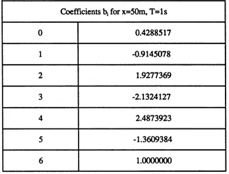
APPENDIX B COEFFICIENTS OF THE RECURSIVE FILTERS FOR THE HORIZONTAL TRANSMISSION OF WAVE MOTION

NOTATIONS

Acronyms

AR Autoregressive model

ARMA Autoregressive - Moving Average model

DFT Discrete Fourier Tranform

FFT Fast Fourier Transform

IDFT Inverse Discrete Fourier Transform

LP Linear Programming

MA Moving Average model

MDOF Multi Degree of Freedom system

MIMD Multiple Instruction stream - Multiple Data stream MISD Multiple Instruction stream - Single Data stream PSD Power Spectral Density function

SLMD Single Instruction stream - Multiple Data stream SISD Single Instruction stream - Single Data stream

TRAM Transputer Module

Symbols

Latin alphabet symbols are listed first, Greek alphabet in the end. Some sym­ bols refer to particular chapters or pages only.

<*i aij bi biJ IB] c,c S lV CKi«2

Ci C(z)

4 D(z)

D

D {l0,6), Z>(0)

Fourier coefficients (Amplitude of a component sine wave) Coefficients of the numerator of a recursive digital filter Gaussian random variable (p. 16)

Coefficients of the denominator of a recursive digital filter Gaussian random variable (p. 16)

Matrix of cofficients (chapter 4) "damping” constants (p. 35)

Covariances between kinematic quantities at two grid

points.

Coefficients of the numerator of a AR or ARMA model z-Transform of the numerator of an AR or ARMA model Coefficients of the denominator of a AR or ARMA model z-Transform of the denominator of an AR or ARMA model Diameter of a cylinder (Chapter 6)

el

fix)

Fft)

8

8 ( k )

G

G(z)

G{ei(*T)

h(t), h(k)

H ( (0)

[H]t [H J, [HJ, [ H J [H(a,b)J

H j 1}(x) H

h J 2 ID

J(a,b)

J J x ) k, k x, k y

k, k

L

m f, m 4*

M N R( Q) R Ryy [ R]

Si coj T

T _{A mux* ■*} T_prod [T(a,b)]

ux, ur u z

Output error measure (Chapter 4) Equation error measure (Chapter 4)

Spatial shape function of an initial disturbance (Appendix) Space-wise Fourie transform of/(x)

gravity acceleration

Impulse response function af a digital filter Constant (p. 35)

z-Transform of a digital filter

PSD of the output of a digital filter

Target Impulse response function

Target Transfer function

Matrix of target impulse response function coefficients, and its partitions (Chapter4)

Hessian matrix in optimization

Hankel function of the first kind, order m, argument x. Significant wave height

Integral (p. 204)

Identification of a processor in a pipeline (Chapter 8) Objective function in minimization algorithms. Bessel function, order m, argument x.

Wave number, and wave number projected to x or y axis

"Spring" constants (p. 35)

Wave length

Third and fourth order statistical moments

Order of the denominator of a digital filter (Chapter 4) Order of the numerator of a digital filter (Chapter 4)

Wave runup on a vertical cylinder at angle 0 Maximum wave runup on a vertical cylinder Auto-correlation function of the output of a filter Diagonal matrix of weights (Chapter 4)

Power spectral density of a random process Time step or digitization interval

Timings of activities (Chapter 8)

ux, u y, u t ... Components of water particle acceleration.

U[0,1 ] ... Random number uniformly distributed between 0 and 1 v ... wave velocity (p. 38)

w(t), Wj ... White noise (continuous or discrete time) w(tjc) ... Two-dimensional white noise

x , X ... Transmission distance

y, Y ... Output time series of a digital filter a ... Parameter (in Chapter 4)

pm ... Complex multiplier for the m-th order term (Chapter 6)

8, ... Unit impulse

e ... Error measure

e ... Small number (p. 203-204)

Wave elevation T|(x,y,r)

0 ... Wind direction

0 ... Integration variable (p. 206)

fynax — Principal wind direction

X ... Scaling factor (Chapter 4) p. ... Mean value of a random process

£ ... Space-wise Fourier transform of x (Appendix A)

p, ... i-th pole of a digital filter

o 2 ... Variance of a random process

T ... Time lag

<}),, <}>,;, ... Random phase of component sine wave

<!>*-> & — Total wave velocity potential, incident and scattered waves’ potential.

co, CD,-, coij ... Frequency, frequency of component sine waves

coc ... Cut-off frequency, Central frequency (p. 105)

CORRIGENDA

Page Line Corrections

2 18 F o r... "forth1' re a d ... "fourth" 17 3 F o r... "into" re a d ... "in"

21 15 F o r ... ”Eq.(2.17)" re a d ... "Eq.(2.15)M 22 9 F o r... "modeling" re a d ... "modelling" 22 16 F o r... "but and" re a d ... "but also" 22 21 F o r ... "Eq.(2.12)" re a d ... "Eq.(2.10)" 23 11 F o r ... ”Eq.(2.13)" re a d ... "Eq.(2.11)" 24 16 F o r... "Eq.(2.24)" read ... "Eq.(2.21)" ■ 40 18 F o r ... "A infinite" read ... "An infinite" 62 1 F o r... "M-l" re a d ... "N-l"

62 1 F o r... "N-l" re a d ... "M -l"

70 11 F o r... "conditining" re a d ... "conditioning" 70 18 F o r... "the the" re a d ... "the"

72 4 F o r... "impovement" re a d ... "improvement" 79 11 F o r ... "minumum" re a d ... "minimum" 79 19 F o r ... "bellow" re a d ... "below"

104 15 F o r... "succesfully" re a d ... "successfully" 113 Fig. 5.10 F o r... "4098" re a d ... "4096"

114,116 3,1 F o r ... "CYLINDRES" re a d ... "CYLINDERS 117 18 F o r... " bm" re a d ... " pm"

120, 122 10,11 F o r... "Eg." re a d ... "e.g." 124 5 F o r... "to" re a d ... "as" 124 14 F o r ... " R(6)" re a d ... " R ”

127 Fig.6.1,2 F o r ... "Scaterred" re a d ... "Scattered" 137 10 F o r ... "terns" re a d ... "terms"

137 13 F o r... "begining" re a d ... "beginning" 139 9 F o r... "are taken" read ... "and are taken" 144 6 F o r... "was" re a d ... "as"

160 11 F o r ... "in" re a d ... "at"

162 3 F o r... "Figs.3" re a d ... "Figs.8.3"

163 1 F o r ... "Alternative" re a d ... "Alternatively" 166 18 F o r... "were" re a d ... "where"

167 4 F o r... "(Hart an" re a d ... "(Hart and" 171 6 F o r ... "2356986" re a d ... "23569856" 172 5 F o r... "programme" re a d ... "program" 172 7 F o r... "into" re a d ... "in"

188 7 F o r... "Spanos" re a d ... "Spanos (1983)" 190 16 F o r... "a Green’s" re a d ... "Green’s" 190 21 F o r... "to" re a d ... "in"

CHAPTER 1

INTRODUCTION

INTRODUCTION

A. The research topic - Approach

A reliable analysis and design of structures subjected to adverse environmental conditions, such as wind loads, earthquakes or sea waves, would require an accu­ rate description of the loading process. This would be possible if precise models for the generating mechanisms existed, which is not the case for most situations. A deterministic analysis therefore can be performed under idealized load patterns only. This is the approach adopted for example by most building codes for the case of earthquake and wind loads. A second approach is to derive the frequency

domain statistical properties of the loading process from recorded data and then perform a random vibration analysis to calculate the response of the structure from input-output relations. However, this method would yield accurate results only for linear systems. When nonlinearities come into play, either in the description of the structural system, or in the loading process, as it may be required for limit design reliability assessments or fatigue analysis, certain, sometimes severe, approxima­ tions will have to be adopted, and nevertheless the problem becomes theoretically quite complicated. Monte Carlo simulations can then be used as a reliable but usually computationally expensive alternative. A family of time domain realiz­ ations of the process are applied to the structure and a deterministic non-linear analysis is used to derive the response. Response statistics on the ensemble can also be evaluated and compared with approximate theoretical solutions.

response as well of a structural system must be accounted for. The basic aim of this thesis is the development of algorithmic tools for the generation of very long, uninterrupted, records of wave kinematics, from which the wave force time histories can be derived These can then be used as excitation inputs

simultaneously at different locations of an offshore structure.

The sea surface can be considered as a random field The laws of hydrodynamics impose a certain functional form on the correlation structure of the random field The majority of the simulation methods which are found in the literature represent the wave’s random field using multidimensional or multivariate models which are based exclusively on matching the prescribed correlation structure. Little use is made of the propagation laws of the underlying medium.

A different approach is attempted in the present work. The aim is to derive the transmittance or transfer function of the medium from the knowledge of the wave motion at certain locations. The problem is similar to the initial value problems encountered for example in geophysics when using seismic exploration for petroleum prospecting. There, the aim is to deduce the earth's properties from measurements on the surface. Also in seismology the generating mechanism of earthquakes is frequently deduced from recorded seismograms on various locations. The basic principle is common in these applications and goes back to optics; the differential equation of the wave motion is used to derive, employing wave extrapolation methods, the transfer function of the medium. In some cases the solution is known and the required function can be easily acquired. For example in the case that is dealt in this thesis the incorporation of Airy’s linear wave theory facilitates the extraction of a transfer function for the transmission of wave kinematics between two points. The corresponding impulse response

function of the medium can be subsequently derived and used for convolutions in

the time domain. However, if the solution is not known, the initial value problem is solved by treating the differential equation either by approximations, or by finite difference methods. An attempt to derive the impulse response function by solving an initial value problem and using approximations to the hydrodynamical

equations is presented in an Appendix. The outcome of this alternative approach is comparable with the one used in the main body of the thesis.

The existence of a large body in the sea, a structural element of an offshore structure with significant horizontal dimensions is an example, modifies the wave field around it. The principles used for the simulation of the undisturbed field still apply and it is possible to derive a transfer function that incorporates the effect of this disturbance in the generation of the kinematic quantities at various locations in the vicinity of the body. This application will be considered in the thesis as well Once the impulse response functions which are required for the time domain convolutions are obtained, the corresponding digital filters must be designed. Computational economy is a factor of major consideration in Monte Carlo

simulations, and in particular in the present scheme where a substantial number of convolutions must be performed in order to reproduce the wave field. Thus the design of efficient and economical digital filters for the simulation of the multi-directional wave kinematics is a primary target of this thesis and will be examined thoroughly.

programmer. The study of the performance of a parallel implementation of the simulation scheme will take a significant position in this thesis, and its

optimization will be pursued.

B. Outline of the chapters

In the following the structure of the Thesis is presented in terms of the contents of its Chapters.

In Chapter 2 a critical review of the methodologies used for the simulation of random waves is presented. The sine wave superposition methods are presented, but particular attention is given to the digital filtering methods. The methods for the simulation of the multi-directional wave kinematics are examined separately. Analogies and differences are drawn with regard to the scheme that will be used in the thesis.

Chapter 2 starts with the presentation of the method used for the generation of wave motion at one point in the sea and then proceeds with the description of the method which uses propagation filters and convolutions to generate the whole directional wave field. Different impulse response functions are used for the generation of the various kinematic quantities and design aspects are considered. The need for the design of low order filters for the horizontal transmission of elevation is identified.

In Chapter 4 optimal recursive digital filters are designed in the time domain in order to replace the infinite length impulse response function used for the horizontal transmission of wave elevation. Special attention is given to this function because of its complicated functional form and the generally high order filters that it spawns. Optimization methods borrowed from digital signal

processing are used in the design.

For completeness of the design aspects, Chapter 5 presents an attempt to design the recursive filters for the horizontal propagation in the frequency domain with the use of allpass filters. The properties of these filters are examined in some detail. Bandpass filtering is also introduced for some case.

In Chapter £ the modification of the wave field around a large cylinder is examined and an impulse response function for the scattered waves is derived. Digital filters are created that together with the filters for the incident waves designed in previous chapters, can reproduce the wave field around the large body. The wave runups are examined and compared with theoretical values.

In Chapter 7 the sequential program written to implement the simulation scheme is presented and the quality of the generated time series is demonstrated in terms of their statistical properties. The unidirectional and the multidirectional cases are examined separately.

Chapter 8 presents the parallel implementation of the simulation program. Various topologies are tried. The performance of the distributed program is monitored using timing devices implanted in the actual code. As an independent check, a simulation of the performance of the program is accomplished, employing a proprietary package. A real time visual display is implemented as well.

Finally in Appendix J£ the coefficients of the recursive filters designed in Chapter 4 are listed for possible use by prospective users of the proposed simulation scheme.

CHAPTER 2

CHAPTER TWO CONTENTS

2.1 Introduction ---- --- --- 15

2 2 Superposition of sine w av es.________________________________ 15

2 3 Digital Filtering m ethods._______ 18

23.1 Univariate digital sim ulation. ... ... 19

i. Autoregressive models 20

ii. Moving average models 22

iii. Autoregressive - Moving average models. — 23

23.2 Multivariate and multidimensional digital simulation. ... 25 Autoregressive - Moving average models. ___ 28

2.4 A hybrid m ethod. ... 30

SURVEY OF THE METHODS FOR THE SIMULATION OF RANDOM WAVES

2.1 Introduction.

Although a variety of methods for the synthesis of random wave kinematics have been developed in the last three decades, they can nevertheless be divided into two broad categories: the summation of sine waves methods and the digital filtering methods. The basic features of these two groups will be examined in the present chapter. A more detailed presentation of the digital filtering methods is undertaken because the simulation scheme used in this thesis falls in this category. The

method of Local Average Subdivision, proposed very recently (Fenton and Vanmarcke 1990) for the simulation of homogeneous random fields, is more suit­ able for finite element models and is not examined here. Furthermore, a method that combines elements from both main categories is included at the end of this chapter.

2.2 Superposition of sine waves.

The summation of sine waves method was proposed in the early sixties for the simulation of random processes and it has been widely used since then (Borgman 1969,1979), (Shinozuka and Jan 1972), (Elgar, Guza, and Seymour 1985), (Wang 1986), (Miles and Funke 1987), (and in Schueller and Shinozuka 1987). In its simplest form, the single summation model, the elevation at a point in the sea is the superposition of a large number of single harmonics:

where A, = V25(g>»)Ag) and <J), = 2jtf/[0, 1]. In this model the only random

element is the phase, uniformly distributed between 0 and 2tc. The amplitude is derived from a target spectrum, like Pierson-Moskowitz, Jonswap etc.

This model can be easily extended to the multidimensional case to include direc­ tional waves. A double summation over harmonics and directions gives the wave elevation as:

n u (2.2)

r\(x,y,t) = .2- 1 cosCco^r - k^x cos 0; + y sin 0;) + fy) f = 0 ,7 \2 7 \ 3 T ,...N T

In the above equation the coefficients Aiy and <J>y can be determined in two ways. The phase only can be random, as in the single dimension model:

AtJ = V25(co.,e,)AcaAe and % = 2jtt/[0,1] (2-3) or both phase and amplitude:

= and <t>,, = (2'4)

where au and 6iy are Gaussian random variables with variance 5(od„ 0,)AcoA0.

The directional spectrum firom which these quantities are obtained is given by the relation:

5(G)i,0y.)=D(G),.,0>)5(G)i) (2.5) where D (co,, 0y) is the spreading function.

Problems with the above models have been reported extensively. Jefferys (1987) points out the ’’phase locking" effect, "due to wave components travelling in different directions with identical frequencies". This results in wave fields that are neither ergodic nor homogeneous.

Alternative methods have been proposed to overcome the phase locking effect The single direction per frequency model (Miles and Funke 1987):

N M (2.6)

T1 (x ,y ,t)= 'L X A ■ cos(co^r- k~(xcos0 .+ y sin 0 ) + <y r = 0, T ,2 T ,3 T ,...N T

where in every frequency interval all the component waves from different direc­ tions have different frequencies respectively, and the much simpler single summa­ tion model (Miles and Funke 1987), (Lando, Scarsi and Taramasso 1991):

N (2.7)

Tl(x,y,r) = X A, cos(co,r - kL(x cos 0*+y sin 0.)+<{>,) is 1

f = 0 ,T ,2 T ,3 T ,...N T

which requires fewer components than the double summation and also avoids phase locking. M directions are considered in each frequency interval Aco, and N frequencies in the band of interest In a modification of this model (Miles and Funke), the frequency and direction components are given as:

Using this technique, each wave train (direction) contains N frequencies which are different from the ones included in any other wave train. Much shorter record lengths are sufficient to generate spatially homogeneous seas. Miles and Funke however suggest caution when using this method because it exhibits a variability which is inconsistent with real seas.

Any model that belongs to the summation of sine waves class can be interpreted as an inverse Fourier transform operation from frequency domain to the time domain; it is known that the computational effort involved is of the order of Nlog2(N) with the best of available algorithms and that the storage requirement is proportional to N. On the other hand the digital filtering method involves a computational effort linear in N, and a very small amount of storage. While the comparison of the oper­ ation count does not show a pronounced advantage for the filtering method (putting aside the issue of numerical stability of the FFT method at very large N), the difference in storage requirements is decisively in favour of the filtering method.

2.3 Digital Filtering methods.

Digital filtering is already an accepted method in the synthesis of random waves in model tanks (Biyden and Greated 1984), (Bryden and Linfoot 1991), (Nunes 1987). However, until recently, the limitations of central computing facilities have militated against the use of this method in theoretical research, and the summation of sinewave components method has prevailed. The batch mode of job execution, common on large Mainframe computers, creates a preference towards multiple finite tasks as opposed to single continuous runs. Interactive time-shared Main­ frame computing has not changed this position because indefinitely long runs are impractical in time-sharing environments. The advent of standalone office

computers, and more recently, the introduction of parallel computing facilities on such equipment, have made digital filtering an attractive proposition. Although proposed as early as 1972 (Burke and Tighe 1972), the method has not gained wide currency until nearly a decade later (Spanos and Hansen 1981), (Samii and Vandiver 1984), (Lin and Hartt 1984), (Mignolet and Spanos 1987).

The basic idea in this class of modelling is to construct a digital filter, or a "black box", to which the input is a sequence produced by a random generator, usually Gaussian white noise, while the output time series matches prescribed statistical characteristics. The aim of the design is to estimate the coefficients of these filters, using the lowest possible order.

We will distinguish between univariate digital filtering methods, where time series are generated at one point in die sea, such that their spectrum matches a "target", and multivariate or multidimensional, where the whole random field, in other words a whole area of the sea surface, is simulated. The first class will be first reviewed in some detail.

2.3.1 Univariate digital simulation.

Employing techniques used in time series* analysis, three main models of digital filters for random process simulations have been used. Autoregressive (or AR, or all-pole) models, moving average (MA or all-zero) models and the complete autoregressive-moving average model (ARMA). The univariate version of these models will be presented, as this will be used in the present work as a first step in the proposed method, although a generalization to the more general case will be included in a following section.

For the autoregressive model:

A Cq

« * (* ) = --- r1

(2.9)

for the moving average:

1 + X dpz~^

5=1

(2.10)

and for the ARMA model:

C(z) £I cEz"*

u , , N _ i d £ 2 _ _ _________

n ARMA\Z ) ~ n ( . \ ~ *

D{Z) 1 + 1 d x *

S=1

(2.11)

In the following the methodologies that have been used for the estimation of the coefficients of these models will be discussed.

i. Autoregressive models.

The difference equation that yields the value in the present time of the output Y of the AR filter (or all-pole filter) when the input is white noise is given by the relation:

- „ * „ (2.12)

y / = y (/r) = c0w/ - i d ^ 5=1

where T is the time step (or sampling period). Multiplying both sides of the equation by Y(l - k ) and taking expectation one gets:

% ( /) + i - / ) = C j t f w ( l ) / = 0,±1,±2,...

where R ^ is the auto-correlation function of the AR process, and R^w is the input-output cross-correlation function.

The coefficients of the AR model will be estimated so as to minimize a

measure of the error between the target PSD and the spectrum of the generated time series (Spanos 1983):

where G(e,aJ) is the power spectrum of the output of the AR filter. Using Maximum Entropy methods (MEM), it is proved (Mignolet and Spanos 1987) that the minimum error is achieved when the coefficients d* satisfy the

following equations:

which are the well-known Yule-Walker equations. In this set of equations Ryy is the auto-correlation function of the target process and is obtained as the inverse Fourier transform of the target PSD, discretized at the required time-lags. Once the dj coefficients are determined from Eq. (2.17), coefficient Cq can be

obtained by equating the target and the AR auto-correlation functions at all the desired time-lags:

and then substituting, together with the estimated coefficients dj, in Eq. (2.15) to yield the solution:

(2.14)

T

« „ ( / ) + ! - 0 = 0 / = 0, ±1,±2, ... (2.15)

(2.17)

In various papers (Spanos 1983, Rivero 1987) directives can be found on how to proceed, step by step, to the methodology outlined above. Details such as how to estimate the order N of the AR model or how to avoid the possible ill-conditioning of the matrix of auto-correlation values (Toeplitz matrix) in the Yule-Walker equations can be found there.

Once the AR coefficients have been estimated, time ordinates of the process Y can be generated recursively using Eq. (2.14).

The AR modeling of a random process offers the advantage of its relative simplicity in the estimation of the coefficients and furthermore the solutions obtained from the methodology described here are guarantied to yield stable filters (Rivero 1987). However, the order of the filters obtained this way is usually high, making their use quite costly in computational terms. In fact Spanos (1983) has observed that in order to reproduce the peakedness of die target spectrum (Pierson-Moskowitz) the order of the AR filter must not be small (but also not too high). Another significant limitation is that they cannot accurately model processes whose PSD has a zero at the origin of the © axis because the all-pole transfer function does not possess a zero.

ii. Moving average models.

The transfer function of the MA model, also called all-zero or FIR (Finite Impulse Response) model, was given in Eq. (2.12). The difference equation used to obtain the MA time series from white noise input is:

ft *nkT)=i_c,wt_l

In this equation an infinite number of weighted white noise ordinates is used in the right hand side, but in practical applications a finite order of the MA coefficients, M, is sufficient

As in the AR case the coefficients are estimated so as to minimize a measure of the error between the PSD of the generated time series and a target PSD. Since MA modelling was not used in the present work, details will not be given here, but can be found in various publications (Haykin 1979,1983).

iii. Autoregressive - Moving average models.

In ARMA modelling both the poles and zeros of the transfer function in

Eq. (2.13) must be estimated, thus making the design a rather complicated task, and moreover sometimes unstable. Nevertheless the computational economy attained by the use of the generally low-order ARMA filters render this approach very popular.

The corresponding difference equation is given by:

Various methods have been proposed for estimating the coefficients of this model. The most straightforward is to extend the logic of the AR estimation, in other word minimise an error measure between the PSD of the generated time series and the target*

(2.19)

'ARMA

G ^ ( e ,or)

If the PSD’s in the above equation are written in terms of the corresponding transfer functions //(©) and HARMA{.e'air) = C(etaT)/D (e,wT\ one obtains an equivalent error measure:

(2.21) e ^ = J j « ( “ )0 (e " ) ~ C («'i“r) I2 d a

In order to minimize e from the above equation directly, a set of non-linear equations in c{ and 4 have to be solved. Most techniques developed to by-pass the nonlinearity involve a two-stage approach. An AR model is designed first according to the method described earlier. Subsequendy this solution is used, in different ways according to the method followed, to estimate the ARMA coefficients.

According to Rivero (1987), an AR model is designed from the given second order information (target spectrum --> auto-correlation) using Maximum Entropy Methods. An impulse response function approximation to this AR filter is then obtained, which is used together with the given auto-correlation, in a second order minimization to estimate the coefficients of the ARMA filter. After some manipulation of Eq. (2.24), the error that will be minimized is given by:

* "* * o (2.22)

e= I i - j \ ) ~ £ ( £

i , y * 0 J J = 0 y = 0

where h is the impulse response function of the AR model. This minimisation can be performed using iterative methods, or solving a system of equations, from which the coefficients ^ are determined. The coefficients c{ can thereafter be estimated by straightforward calculations:

n

C: = £ rfA--# ^or i = 0,1,2,.. .m

>-o

(223)

This method appears to be quite suitable and yielding satisfactory results for univariate ARMA modelling of sea waves [Rivero], but is not known to cope with the more general multivariate case. A quite different approach to the univariate ARMA filter design which uses an intermediate analog filter was propose by Spanos (1983), but will be presented in a subsequent chapter in detail, as it is the method used in this work for the generation of waves at one point in the sea.

2.3.2 Multivariate and multidimensional digital simulation.

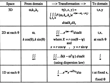
It is important to distinguish between general random field simulations and the simulation of random wave fields obeying linear wave mechanics in a disper­ sive medium. In the former case the appropriate digital filter is three dimen­ sional, two space and one time, or multivariate if the space points are absorbed into elements of a vector, (Mignolet 1987), (Samaras, Shinozuka, and Tsurui

it utilises the medium’s wave propagation law in the design of the filter. Table 2.1

Space From domain —> Transformation —> To domain

3D _(nXxky

1

J

d(adkydkx

u , y

2D at each 6

kcos(0),fcsin(0)

JJ

where X = r cos(0 - y) and

x = r c o s y , y = r sin\{/

at each 0

jj

C D *

J J

.. -5(Jfe

- to2/*) dead*

a>k

(using dispersion law)

j o

ID at each 6 l ...e ‘"e~i'°lxi,d(a

CD

t at fixed x, fixed 6 An example of two-dimensional linear filtering is the system used by Bryden and Greated (1984) for the generation of waves in tanks. The desired output is given by the convolution:

(2.24)

where the input is a two-dimensional white noise w(t,x). The impulse response function of the filter, h(x,X), is determined from the inverse Fourier transform of the system’s transfer function:

(2.25) h(z,x) =

j j~

This function is then either digitized and truncated in order to produce the required digital filter, or used directly in the convolution described by equation (2.9) to generate the desired output. As far as digitization is concerned, it should be noted that there exist more elaborate techniques (see chapter 3) than the ones used by the authors, which would improve the quality of the output As for the transfer function, it is obtained from the square root of the target directional spectrum.

where use of the dispersion relation has been made, and W is the intensity of the input white noise spectrum.

As pointed out by the authors (Bryden and Greated 1984) spectra do not carry phase information, and thus an arbitrary choice has to be made with regard to the phase. Although the cross-correlations of the generated series appear to match theoretical values, there is no indication that the correct phase relation between separate points in the sea is retained. It should be noted that this criti­ cism is valid for all the methods that are based on correlation matching, and will be reviewed next

In the following we will examine the multivariate ARMA models, since the methodologies used for the multivariate AR or MA models are analogous to those for the corresponding univariate models examined earlier. In the ARMA models the similarities are still present, but the handling of the matrix and vector formulations is more delicate and needs some attention.

Autoregressive - Moving average models.

A multivariate ARMA process f can be generated from previous values and multivariate white noise input Wt according to the equation:

. " » - (2.27)

t = ' L C lW,_l - Y . D tt _ l

I* 0 * » 1

where C, and Dk are the coefficient matrices, n x n for an n-variate process.

In order to determine the coefficient matrices of this ARMA model Mignolet and Spanos (1987), adopting a two-stage approach familiar from the univariate case, design initially an AR model and then use its transfer function to

approximate the denominator of the ARMA model. The error to be minimized is an expression of the coefficient matrices Ct and Dt of the system, the

auto-correlations of the output process and the cross-correlations Ryw of the AR system:

* n ft in (228)

e = I XD fiff(k — i)D/ — X XD f i t ^ k - l ) C \

* = 0 » * 0 k * 0 l * 0

- X X c f l t v i k - i 'p l + i n r r i c ;c ;

* > 0 / * 0 1 * 0

where1 denotes the transpose of a matrix or a vector, while T is the sampling period. Two methods are proposed for the minimization of this expression, a more straightforward auto cross-correlations matching procedure (ACM), which is an extension of the techniques used in AR modeling, and a power order matching procedure (POM), where the numerator of the frequency

domain transfer function of the ARMA nodel, C(etaT), is presented as a Fourier approximation to the product //(co)D (e,aT) (see Eq. 2.21), of order n+m. The Ct and D{ are estimated so as to match the Fourier coefficients of the two

expressions. The authors point out that these two methods are equivalent, but the latter is computationally more efficient. More details on this method can be found in (Mingolet and Spanos 1987). Samaras (1983) uses similar methods for determining the coefficient matrices of his multivariate ARMA model.

Although the previously described methodology is mathematically rigorous in its theoretical form, in practice the handling of large matrices for the

determination of the coefficients of the multivariate ARMA filter may lead to computational difficulties. In order to simulate a extensive area of the sea surface, one would have to construct a filter that would incorporate a large number of locations (variables) thus leading to matrices of high orders. The authors present a quite extensive treatment of the stability of these filters but nevertheless restrict themselves to applications that require low order matrices. An additional reservation is that a simulation method which relies entirely on matching the statistical properties of the generated waves, neglects the physical properties of the underlying medium, that is die mechanics of wave

propagation. This reservation will be elaborated in subsequent chapters.

2.4 A hybrid method.

Before closing this chapter a third, hybrid method of synthesizing random waves should be mentioned which combines Fourier transforms and linear filtering (Li and Kareem 1989), (Kareem and Li 1991). A large number of time series segments is generated using FFT techniques (summation of sine waves), and at second stage digital filtering is involved to synthesize these segments in to a final time series of long duration. This method is extended into the multivariate case using stochastic decomposition to construct the component random subprocesses' desired

simulation. The authors of this technique claim that they can combine the simplicity of FFT methods with the computational economy of linear filtering, since they can avoid the large storage requirements of the former.

CHAPTER 3

CHAPTER THREE

CONTENTS

3.1 In troduction. ______ 33

3.2 Organisation of the simulation scheme (directional w aves) 34

3 3 Generating the surface elevation process at the reference n o d e 34

3.4 Convolution integrals for the transmission of wave kinematics. ... 38 3.4.1 The impulse response function for the sea surface elevation ... 41

3.4.2 The generation of velocity and acceleration time histories. ... 42 A. Vertical water particle velocity._________________________ 43

B. Horizontal water particle velocity. ... 45

C. Acceleration records. ... 47

3 3 Vertical attenuation of wave m otion._________________________ 47

3.6 Multidirectional case._________________ 48 3.6.1 Rounding errors. ... ... 49

THE USE OF PROPAGATION METHODS FOR THE GENERATION OF WAVE

KINEMATICS.

3.1 Introduction.

The basic principle behind the simulation method described here is the acquisition of the transfer function for the propagation of the various wave kinematical quantities in an elastic medium from the knowledge of the wave motion

characteristics at some points. The motion at any desired location can thereafter be obtained using convolution integrals. The method is similar to techniques used in optics, geophysics and seismology.

3.2 Organisation of the simulation scheme (directional waves)

The following flow chart assumes that wave kinematical quantities are required at points of a 3-dimensional grid covering an area of interest

Do for successive time steps: Do for all wave directions:

1. Produce one step of the input white noise process. 2. Generate one surface elevation process value at the reference node.

Complete over the directions. Do for all grid points:

Do for all wave directions:

1. Transfer by linear digital filtering to elevation, velocity vector components, and acceleration vector components at all other nodes

2. Add directional contributions Complete over the directions. Do for all depths

Transfer, using attenuation filters Complete over depths

Complete over grid points Complete all time steps.

In the following the steps of this scheme will be examined one by one. Although the final simulation package is multidirectional, the unidirectional case will be assumed first, which will be extended to the more general case in the end of this chapter.

3.3 Generating the surface elevation process at the reference node

Filters may be designed for a white noise input such that the output process has the desired autocorrelation function (or equivalently, autospectrum). Gersch and

co-workers have presented a two-stage procedure for digital filter design, both in the univariate and the multivariate case (Gersch and Liu 1976), (Gersch and Yonemoto 1977). Also see Samaras, Shinozuka and Tsurui (1985).

A filter design scheme specifically aimed at simulating wave motion by means of an autoregressive-moving average (ARMA) model has been developed by Spanos (1983). In the present study that scheme is adopted as the generating mechanism for the random process at the reference node. An ARMA model has the following power spectrum (Papoulis 1984):

The coefficients q and dj must be determined in such a way as to make the power spectrum of the output process approximate the desired spectrum, e.g.

Pierson-Moskowitz. Spanos accomplished this task by introducing an intermediate process whose output has the power spectrum:

which represents the transfer function of a cascade of two linear systems in terms of their "spring and dashpot" constants.

The coefficients G, c, k etc. are determined by minimizing the residual error, in a least squares sense, between the target process and the power spectrum of Eq. 3.2. The time-domain differential equation which would yield this type of process from a white noise forcing function is easy to identify, and may in turn be used to find the Laplace Transform-transfer function involved. Finally using the approximate

(3.1)

1 + I d p -* *

2

technique of bilinear transformation, the s-transform is converted to a z-transform, which is the required filter of Eq. 3.1. In this way the following coefficients Cj and dj for H(z) have been obtained from Spanos* expressions:

Here T is the fundamental time-step of the digital filter. In general, if co* is the bandwidth of the spectrum to be matched, then T must be chosen less than ti/cd*. However Spanos recommends using a time step 4 times smaller than this limit in order to compensate for the error caused by the bilinear transformation.

Once the coefficients c4 and d* have been determined, the recursive filter equation which will generate the output process from white noise input w is:

It should be noted that Sorensen and Thoft-Christensen (1985) have developed an alternative algorithm for the simulation problem under consideration: this relies on

c0 = / dl = 2 ( - 2 p - r + v+2q)IS q = 0 d2 = 2(3p - u + 3q)/S

c2 = - I f d3 = 2(-2p + r -v + 2 q )/S c3 = 0 dA = (p - r + u - v + q ) / S C4=f

where: (3.3)

p - 1 6

r = 8 a7 $ = k + k + cc w = 4 p 7 2 y = c k + ck v = 2 y T 3 £ = kk

a = c + c

f = 4-jG T2/S

Y, = Y(IT)=

I

E

S * *

m n _(3.4)

a transformation from a n-dimensional Markov vector random process to a final non-Markov process which is ARMA, of order n x m , and was reportedly proposed by Franklin. Sorensen and Thoft-Christensen have fitted the power spectrum of the output to both Pierson-Moskowitz and Jonswap spectra. The computational cost of this method is likely to be comparable to the former approach. In the present study it was decided to use Spanos* approach simply because more information was available on coefficient values fitting the model to various wave spectra.

In this study the Gaussian variates needed for the white noise input process have been generated by a procedure proposed by Ahrens and Dieter (in Bratley, Fox, and Shrage 1985) (algorithm L19) This is a composition method for generating standard normal variates. The total area under the standard normal

probability-density curve is partitioned into a large trapezoidal subarea and four odd-shaped small subareas. Each subarea is treated as a density distribution. Random variates are chosen from the respective distributions, with probabilities proportional to the distributions* enclosed area.

The U(0,1) random variates required in this procedure are drawn from a uniform random number generator. The algorithm used in this report belongs to the class of multiplicative generators with prime modulus (algorithm L20 in Bratley, Fox and Shrage).

3.4 Convolution integrals for the transmission of wave kinematics.

In order to transfer the motion of the sea from the point where it was generated to another, the Duhamel convolution integral can be used. The generated time series at a point can be treated as a series of input displacement impulses, and the impulse response of the sea surface may be used to transmit this input to the second point To accomplish this task, the transfer function of the sea surface must be sought first

The transfer function can be obtained using methods generally described as wave extrapolation. Numerical or analytical procedures can be employed in wave extrapolation. It is worth presenting here in brief an optical application, described by Claerbout (1985). The problem there, is to project waves across a region of empty space. Using the wave equation in optics, the motion at (t,x,z) is described by the relation:

p (f ,x, z) = P (©, kx1 z y T im^

where the amplitude of the motion P((d,kx,z) at z is related to the amplitude of a disturbance at z0 via the equation:

P (co, kx,z) = P (co, kx, z0)e 1 }

where v is the wave velocity. From the above equation the filter transfer function can be easily deduced:

e x p j i C c o V - ^ A z - z j

Inverse Fourier transforming this relation either in time or space domain or both, a corresponding impulse response function is obtained which can be used in

convolutions.

If analytical solutions of the wave equation do not exist, for example if the velocity v is space variable, numerical wave extrapolation methods are used. Claerbout (1985) describes such a procedure in geophysics.

Coming to the present case of sea waves, linear Airy’s theory is used to express the velocity potential of the surface waves for infinite depth water:

where H is the significant wave height From the above, using a boundary condition to the Laplace equation:

the equation which gives the instantaneous surface elevation, T|, of a propagating single harmonic wave can be given as:

where © is the angular frequency of the wave, k is the wave number, and A - H 12 defines the amplitude. In practice only the real or the imaginary part of the

equation is used.

If a constant amplitude harmonic input of frequency co, x(t), is applied to a linear system, the corresponding output y(t) will be given b y :

qCx ,t) = A e ii°“ kx) (3.5)

where H(co) is the system’s complex frequency response function or transfer function evaluated at angular frequency CD. Taking account of the above equations, and using the dispersion relationship for deep water k = co2/g, the transfer function becomes:

//„_„(o v t) = e 'i<'A ' ' ) (3 J) It is noted that both the real and the imaginary parts of this function are even functions of CO. In general, the inverse Fourier transform of H(co) is h(t). Under the present conditions h(t) would be a complex-valued function. It would not be valid to use the real part of such an h(t) function on its own, since this would not have the necessary frequency-domain properties (its transform would be a purely real-valued H function, giving zero phase). However if the function H(co) were chosen conjugate-symmetric (even real part, odd imaginary part) its Fourier transform would be real-valued. Hence, the following is substituted for Eq.3.7:

a>,x) = e^in ^ A , •

= cos

( 2 >

COX

- i sgn(co)sin . 8 > . 8 > This function is characterized by the two properties:

2

| H(cd)] = 1 and arg [H(o>)] =-sgn(a>)—

8 (3.9)

A infinite length digital filter with these characteristics may be obtained by taking the inverse Fourier transform of the H(co) function given above. This is the method used in the work of Vandiver and co-workers, see Samii and Vandiver (1984), Dommermuth (1986). The infinite length filters are usually truncated to a finite

length. In the present work they will be re-expressed in even more compact form as recursive filters. But first, the full impulse response function corresponding to Eq. 3.8 will be presented.

3.4.1 The impulse response function for the sea surface elevation

The Inverse Fourier transform of H(co) as given in Eq. 3.8 is:

‘ o - s f

Its explicit form may be obtained using the following integrals (Abramowitz and Stegun (eds.) 1970):

J V c o s C V = (3b *0)

and

( % , s o )

where C(.) and S(.) are the Fresnel cosine and sine integrals. Noting that:

J

J

and

J

J

The result is:

hit)= a/ X

\ 2xn cos_{\ 4 x s}

i+c

This function is plotted in Fig. 3.2a. It is interesting that the foregoing function agrees with an impulse response function derived in hydrodynamical theory. This connection is described in Appendix A.

In practice h(t) of Eq. 3.10 will be truncated. This can be achieved either by a sharp cutoff, or the application of a window. If a sharp cutoff is used in the time domain, it results in a ripple effect in the frequency domain (Gibbs

phenomenon). To illustrate this point, the magnitude of the H(cd) function has been obtained as a continuous Fourier transform for two different truncation lengths, 200 sec and 50 sec respectively (Figs. 3.3,3.4). The phase property is affected mostly at low frequencies.

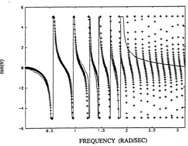
Alternatively, windowing can be performed in the frequency response function. If Eq. 3.8 is assumed zero for | co |> coc, where coc is the cutoff frequency, Eq. 3.10 becomes (Dommermuth):

This function is shown in Fig. 3.2b

3.4.2 The generation of velocity and acceleration time histories.

The generation of velocity and acceleration time histories is necessary for the calculation of the wave forces on the members of an offshore structure, according to Morrison’s formula. Initially forces can be generated at the grid points where elevation has been transferred and subsequently integrated to

yield the total member wave forces. Both components of particle velocity, horizontal ux and vertical and particle acceleration ux and w, should be generated, since members can have varied orientations.

These time histories must be produced by differentiating the elevation time histories with respect to time, for the vertical particle velocity, and then the velocity time histories, to generate acceleration; horizontal particle velocity is similar to vertical, only shifted by 90° in the frequency domain. This technique must be applied with care because differentiation is known to amplify errors (noise) particularly in the high frequency region (Dommermuth). In this application where measured data is not involved, the noise is either due to the difference between the spectrum from the digital filter and the target spectrum (this depends on the quality of the digital filter design), or it is due to roundoff errors in the computer (a remote possibility). If noise amplification is

suspected, the remedy is to generate the elevation time-series with a shorter timestep (higher bandwidth), then apply differentiation and finally apply a low-pass filter in order to retain just the desired bandwidth. However in the present study noise amplification has not been found to be a problem, therefore no special measures are adopted in this respect On the other hand a high performance filter has been used for the differentiation itself, in order to avoid the distortion inherent in the 2-point finite difference approximation.

A. Vertical water particle velocity.

/ / (co) = i co (3.12)

To design a digital filter from this function, its Fourier series representation is evaluated (Chen 1979):

where T is the digitization interval. Integration yields the following h(n):

The above sequence is antisymmetric about zero and tends asymptotically to zero as n tends to infinity, in the positive direction as well as the negative direction. The existence of ordinates for negative n indicates that, unless shifted, it is a non-causal filter. In practical terms this means that when used in a continuous convolution with an input series, some future time steps of the input must be produced and stored in advance. Shifting the filter about its central ordinate in order to render it causal is undesirable because it would distort the phase relation between input and output, which in the present application is important

Since h(n) is of infinite length and decaying, it can be truncated when its value becomes smaller than a fraction of h(l). As usual, this results in ripples in the frequency response behaviour. To overcome this distortion problem the truncated sequence must be multiplied by a time domain window. The Hamming window was used for this particular function (Chen):

(3.13)

h(n) = 0 for n =0 (3.14)

for n * 0

(3.15) w(n) = 0.54+0.46 cos where N = ——

N is the total length of the truncated h(n) sequence. The frequency response characteristics of the windowed filter for the generation of vertical velocity records from elevation inputs is shown in Fig 3.5 (for bandwidth n) and Fig. 3.6 (for bandwidth 2n).

It is worth noting here that the numerical differentiation could have been done with finite difference formulae from numerical analysis. The simplest such scheme is a convolution with the 2-point digital filter:

The frequency response function that corresponds to this filter is (Chen 1979):

which agrees with the correct function Eq.(3.9) only for low frequencies and thus results in large errors for higher frequency components of the input sequence.

B. Horizontal water particle velocity.

A separate digital filter is designed for the horizontal velocity, since its

corresponding frequency response function differs from the vertical case in the phase term (Dommermuth), (Isobe, Kondo and Horikawa 1984):

(3.17)

//*,(©)=! co | (3.18)

one obtains the infinite sequence:

for n = 0 (3.20)

h(n) = 0 for n even for n odd

This is a symmetric sequence of infinite length but decays rapidly due to the quadratic term in the denominator of each term. As in the case of the preceding differentiator, the filter is non-causal due to the symmetry about zero and consequently the same storage technique will be employed when this h(n) is used in the convolutions.

Normally a time domain window would be applied at this point in order to remove the ripples in the frequency domain caused by the truncation; but in this particular case the application of a window has been found to distort the natural kink of the H(co) function at zero frequency. Only when the length of h(n) is large enough, which corresponds to a finer frequency resolution, this distortion will be insignificant, but this is not practical. Fortunately, the function under consideration has a rapid decay even without the use of a window, and the ripples in the frequency response function are of minor order (Figs 3.7 and 3.8). Therefore the h(n) sequence as given in Eq. 3.20 was used for this operation.

C. Acceleration records.

component of acceleration is //. = -co2 (Isobe, Kondo an Horikawa). ***

Alternatively, if the input for the generation of the horizontal water particle acceleration is taken as the horizontal water particle velocity ux, and the input for the vertical water particle acceleration is u,, the transfer function is the same for both cases, namely the differentiator (Eq.3.12). Therefore it is more

convenient in the simulation of the wave kinematics to generate the

acceleration records from the corresponding velocity components, which are generated already, using the same transfer filter for both.

3.5 Vertical attenuation of wave motion.

The five components of wave motion that are initially generated at die surface grid points, namely elevation r|, particle velocity, horizontal if, and vertical u,, and particle acceleration ux and ii„ should be transferred to the grid points in various depths below the free surface to calculate the wave forces on submerged structural members. The elevation record itself is needed at small distances below MWL

where a member can be at times partly submerged, depending on the wave height For deep water, according to Airy linear wave theory, the transfer function for the vertical attenuation for all the wave motion components is (Dommermuth), (Isobe, Kondo and Horikawa):

where dz is the distance below the surface to which the wave motion is transferred. It can be seen that the attenuation of higher frequency components is more

pronounced than that of low frequencies.

T

rr

A(")=W i H r M

where T is the digitization interval. This is a symmetric filter about zero and the discussion in an earlier Section for non-causal filters applies here as well. It should also be mentioned that this sequence decays rapidly (exponentially) and the filters it results in are in general of low order.

3.6 Multidirectional case.

The unidirectional scheme described above can be easily extended to the

multidirectional case. Wave elevation series are generated at the '’reference" point and then transmitted to various points for each direction considered,

independently. The summation of the contributions from different directions is occurring at the points. The wave trains generated at the "reference" point for each direction are uncorrelated, but shaped according to known directional spectra. The directional power spectrum adopted in the present work is given by the relation (Kree and Soize, 1983):

Gm(e,ca)=£>(e,e0)5im(<n) where Z)(e,eo)=A cos*(e-0o) (3-23)

and A is a normalizing constant such that JeZ)(0,8o)d0 = 1, 0O is the principal direction, and n -2.

An example grid used for the multidirectional generation of wave kinematics is shown in Fig. 7.2 of chapter 7.

3.6.1 Rounding errors.

The scheme presented in this chapter requires a set of pre-designed digital filters for each and every filtering operation involved. For the horizontal transmission of wave kinematics a series of recursive digital filters has been designed and is presented in following chapters. These filters cover propagation distances ranging from lm to 50m in intervals of lm. For intermediate

distances, it is proposed to use the filter for the nearest integer distance. This rounding operation by a maximum of 0.5m has an insignificant effect on the cross-statistics of the wave kinematics between two points. Thus, the

covariance of the elevation processes between two points differing by x (unidirectional case) is given, after some manipulation, by the integral:

where 5^(co) is the Pierson-Moskowitz spectrum for the surface elevation process. Similar relations can be written for the velocity and acceleration covariances between two points. In Fig. 3.9 the calculated covariances for distances x (m) and x+OJ (m) are shown superimposed at abscissa x

(continuous lines and markers respectively) in order to display the magnitude of the maximum error due to rounding. Two sets of covariance curves are presented for two extreme sea states, 20 Knots and 60 Knots windspeed. It is apparent that the error resulting from this rounding is in most cases negligible. The error is slightly more pronounced in the case of the acceleration process, for very small distances of propagation. In the multidirectional case, the error is expected to be even smaller, because rounding up and rounding down

It should be noted that in contrary to the horizontal transmission filters, the depth attenuation filters can be designed at run time, and for the exact depth, therefore there will be no rounding error associated with this operation.

S

2

(

W

)

,

D

I

M

E

N

S

I

O

N

L

E

S

S

X 1 0 ' 1

W , D I ME N SIONLESS

THEORETICAL

ARHA TB = T/4 N = 51

1G000 P.

I ~~ T 1 ' ■ I

~-2Q 0 20 40 60 80 100 ”

TIME (Sec)

Fig.3.2.a h(t) function obtained from Fourier transform operation (Eq3.10)

0 .3

0 . 2

-0 . !

- e . 2

60 80

0 20 40

Fig.3.2.b h(t) function from transfer function truncated at coc = 27i (Eq.3.11)

M

A

G

N

IT

U

D

E

MA

GN

IT

UD

E

e.s

- 0 .5

-I

0 .5 2 .5

FREQUENCY (RAD/SEC)

Fig. 3.3 Magnitude of transfer function for the impulse response in Fig. 3.2, truncated at 200 s.

0 .5

0

-- 0 .5

JL iU * o 2 1 ^

: U tb lb H J

05.

05.

1 6 .

Freq (rad/sec)

3

30

27

65

3o28

l o 9 6

67

DIFFERENTIATOR FOR V z , ACC

Fig. 3.5a

DESIGN

99.

33.

33.

99.

3o28

l o 9 6

6.5

6.7

DIFFERENTIATOR FOR V z , ACC

DESIGN

35.

35.

Freq (r a d /sec)

d6 6

59.

13

13

6 6

39

DIFFERENTIATOR FOR VZ, ACC

Fig. 3.6a

: DESIGN

99.

33.

33.

99.

Freq (r a d /se c)

d6 6

39

6 6

13

13

: DESIGN

65.

Freq (rad/sec)

3o30

00

65

‘3d28 "1d96 63

DIFFERENTIATOR FOR Vx

Fig. 3.7a

DESIGN

CL

32.

Freq (rad/sec)

3o30

3 o 28 T o 96 65

DIFFERENTIATOR FOR Vx

: DESIGN

52.

39.

26.

13.

Freq (rad/sec)

^ 6 6

00

o 4 0 X10

13 13

39

66

U)C=6 o 283 N =21o000 DIFFERENTIATOR FOR Vx

Fig. 3.8a

X10-16 l o 4 4 _

~ o 81J

X

£ o29J

_C 0.

a

29-- o 8 1 .

- l o 4 4 .

DESIGN

Freq (rad/sec)

1 1 1 ; ) 1 1 1 1 1

- 0 6 6 — o 39 — o! 3 o l 3 o 40 d 6 6

__________________________________ X-101

DIFFERENTIATOR FOR Vx