R E S E A R C H
Open Access
BicPAM: Pattern-based biclustering for
biomedical data analysis
Rui Henriques
*and Sara C Madeira
Abstract
Background: Biclustering, the discovery of sets of objects with a coherent pattern across a subset of conditions, is a critical task to study a wide-set of biomedical problems, where molecular units or patients are meaningfully related with a set of properties. The challenging combinatorial nature of this task led to the development of approaches with restrictions on the allowed type, number and quality of biclusters. Contrasting, recent biclustering approaches relying on pattern mining methods can exhaustively discover flexible structures of robust biclusters. However, these
approaches are only prepared to discover constant biclusters and their underlying contributions remain dispersed.
Methods: The proposed BicPAM biclustering approach integrates existing principles made available by
state-of-the-art pattern-based approaches with two new contributions. First, BicPAM is the first efficient attempt to exhaustively mine non-constant types of biclusters, including additive and multiplicative coherencies in the presence or absence of symmetries. Second, BicPAM provides strategies to effectively compose different biclustering structures and to handle arbitrary levels of noise inherent to data and with discretization procedures.
Results: Results show BicPAM’s superiority against its peers and its ability to retrieve unique types of biclusters of interest, to efficiently deliver exhaustive solutions and to successfully recover planted biclusters in datasets with varying levels of missing values and noise. Its application over gene expression data leads to unique solutions with heightened biological relevance.
Conclusions: BicPAM approaches integrate existing disperse efforts towards pattern-based biclustering and provides the first critical strategies to efficiently discover exhaustive solutions of biclusters with shifting, scaling and symmetric assumptions with varying quality and underlying structures. Additionally, BicPAM dynamically adapts its behavior to mine data with different levels of missing values and noise.
Keywords: Biclustering, Pattern mining, Biomedical data analysis
Introduction
Biclustering, a local approach for clustering, seeks to find sub-matrices (biclusters), subsets of rows with a highly correlated expression pattern across a subset of columns. Biclustering has been extensively applied in gene expres-sion data analysis [1], since small groups of genes can participate in multiple cellular processes or pathways of interest that may be only active in a subset of the condi-tions under analysis. Biclustering has been also applied to group mutations and copy number variations [2], to ana-lyze biological networks [3], and to study translational [4], chemical [5] or nutritional data [6].
*Correspondence: [email protected]
INESC-ID and Instituto Superior Técnico, Universidade de Lisboa, Lisbon, Portugal
Biclustering involves hard combinatorial optimization. In particular, its complexity increases when rows and columns are allowed to participate in more than one bicluster (non-exclusive structure) and in no bicluster at all (non-exhaustive structure). Hence most existing algorithms are either based on greedy or stochastic approaches [1,2,7,8], potentially producing sub-optimal solutions, or on finding a constrained number, structure or type of biclusters [1,2,9].
The state-of-the-art attempts to tackle biclustering using pattern mining techniques allow for exhaustive and flexible searches and show solid levels of efficiency [10,11]. The fact that pattern mining research is driven by scalability requirements [12], opens a critical direction to
perform biclustering. Interestingly, the existing pattern-based approaches for biclustering – such as BiModule [13], DeBi [10], RAP [14] and GenMiner [15] – pro-vide complementary principles of interest for this field. However, these principles are not yet integrated. Addi-tionally, existing approaches only discover biclusters with constant profiles [10,13,14], and are not able to han-dle missing values or medium to high levels of noise. This work aims to target these limitations by propos-ing a pattern-based biclusterpropos-ing approach, BicPAM, that is able to combine existing potentialities from state-of-the-art pattern-based approaches with two critical novel contributions:
– flexible exhaustive solutions: arbitrary number of (potentially overlapping) biclusters with additive, multiplicative and symmetric assumptions using multiple ranges of values;
– biclustering behavior dynamically adapted to deal with varying levels of noise and missing values.
To our knowledge, this is the first biclustering approach that is able to support and combine each of these two contributions. The importance of these contributions is shown experimentally over synthetic and biological data. Additionally, experimental results on both synthetic and real datasets demonstrate the efficiency and effectiveness of the pattern-based biclustering algorithms proposed in BicPAM.
The paper is organized as follows. Backgroundcovers essential concepts from biclustering and pattern mining, and surveys the contributions from existing pattern-based biclustering approaches. BicPAM: pattern-based biclus-teringdescribes the proposed algorithms. In Results, we assess BicPAM’s performance on synthetic and real data. Finally, the contributions and implications of this work are synthesized.
Background
This section introduces fundamental concepts of biclus-tering and pattern mining, and surveys the related work on pattern-based biclustering.
Definition 1.Given a matrix, A=(X,Y), with a set of rows X = {x1, ..,xn}, columns Y = {y1, ..,ym}, and elements aij∈Rrelating row i and column j:
– A biclusterB=(I,J)is ar×ssubmatrix ofA, where
I=(i1, ..,ir)⊂Xis a subset of rows and J=(j1, ..,js)⊂Yis a subset of columns;
– Thebiclustering taskis to identify a set of biclusters B= {B1, ..,Bp}such that each biclusterBk=(Ik,Jk)
satisfies specific criteria of homogeneity, where
Ik⊂X,Jk ⊂Y, andk∈N.
Approaches to solve the biclustering task either explic-itly or implicexplic-itly rely on a merit function to define the homogeneity criteria. An illustrative function is the vari-ance of bicluster’s values. Merit functions either guarantee intra-bicluster homogeneity, the overall homogeneity of the output set of biclusters (inter-bicluster homogeneity), or both. When combined within specific search proce-dures, merit functions are to define the type, quality and structure of biclustering solutions [1].
Merit functions can be defined to locally maximize greedy iterative searches [7,8,16-19], to combine row- and column-based clusters [20-22], to exploit matrices recur-sively [23], and to stochastically model the target solution [6,24]. In exhaustive searches, which commonly rely on constrained formulations, merit functions are the heuris-tics that guide the space exploration [9,25].
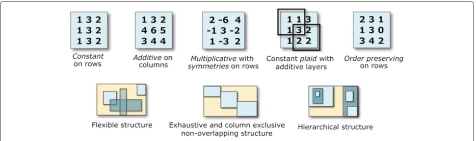
Figure 1 presents different types and structures of biclusters. Biclusters can follow constant or more flex-ible models, with coherency on rows or columns [1]. Biclusters under an additive-multiplicative model, also referred as shifting-scaling biclusters, can be discovered using merit functions based onδ-offsets of noise [17,25], on vector-angle cosines [21], or on generative models of linear dependencies [2]. Biclusters with symmetries can be discovered by differential biclustering methods [9,26] and by few others [14]. Additionally, plaid [6] and order-preserving [19] types of biclusters have also been tackled [27,28]. Multiple biclustering structures have been proposed [1], with some approaches constraining them to exhaustive, exclusive, non-overlapping structures, and others allowing more flexible structures with arbitrarily positioned overlapping biclusters [7].
Pattern mining
Patterns are itemsets, rules or substructures that appear in a dataset with frequency no less than a specified threshold. Finding patterns is critical to derive relations from data.
Definition 2.LetLbe a finite set of items, and P be an itemset P⊆L. A transaction t is a pair(tid,P)with id∈N. An itemset database D overLis a finite set of transactions
{t1, ..,tn}.
Definition 3. A transaction(tid,P)contains P, denoted P⊆ (tid,P), if P⊆ P. The coveragePof an itemset P is the set of all transactions in D in which the itemset P occurs:
P = {t ∈ D|P ⊆ t}. The support of an itemset P in D, denoted supP, can either be absolute, being its coverage size
|P|, or a relative threshold given by|P|/|D|.
Definition 4.Given an itemset database D and a min-imum support threshold θ, the frequent itemset mining
(FIM) problem consists of computing the set {P | P ⊆
Figure 1Illustrative bicluster types and biclustering structures.
A frequent itemset is an itemset with supP ≥ θ. An
accepted pattern is a frequent itemset that satisfies any other placed constraints overD.
To illustrate these concepts, consider the following itemset database, Dex ={(t1,{B,E,G}), (t2, {A,B,C,E,H,J}), (t3,{A,B,D,H,J}), (t4,{D,H,J}), (t5,{A,H,J}), (t6,{A,G})}. We have|L| = |{A, ..,J}| =10,{B,J}= {t2,t3}andsup{B,J}=
|{t2,t3}|/6 = 0.(3). For θ = 4, FIM tasks returns {{A},{H},{J},{H,J}}.
Since FIM proposal [29], multiple extensions have been proposed, ranging from scalable data mining method-ologies to multiple condensed and approximated pattern representations.
Definition 5.Given an itemset matrix, a support thresholdθ, and the coverage function: 2L →2Dthat maps an itemset P to its set of supporting transactions:
– A frequent itemsetPis an itemset that satisfies |(P)| ≥θ;
– A closed frequent itemset is a frequent itemset with no superset with same support∀P⊃P|P|<|P|; – A maximal frequent itemset is a frequent itemset with
all supersents being infrequent,∀P⊃P|(P)|< θ.
A frequent itemset is maximal if all its super-sets are infrequent, while it is closed if it is not a subset of an itemset with the same support. Con-sidering the previously introduced itemset database Dex, a given threshold θ = 3 and |P| ≥ 2, there is one maximal frequent itemset ({A,H,J}) and there are two closed frequent itemsets ({A,H,J} and {H,J}).
Definition 6.Consider two itemsets P ∈ 2L and P ∈ 2L, where P⊆P, and a predicate M. M is monotonic when M(P)⇒M(P)and M is anti-monotonic when¬M(P)⇒
¬M(P).
These properties are the basis of FIM, either for candi-date generation or pattern growth methods, with horizon-tal or vertical data formats.
Pattern-based biclustering
The homogeneity criteria (Definition 1) in pattern-based approaches for biclustering is obtained through sup-port and confidence-correlation metrics. Pattern-based approaches allow for an efficient and exhaustive space search that produces an arbitrary high number of biclus-ters within a flexible structure.
Definition 7.Given a matrix A and a minimum support thresholdθ, a set of biclusters∪kBk, where Bk = (Ik,Jk), can be derived from the set of frequent itemsets∪kPk by either mapping(Ik,Jk) = (Pk,Pk)to compose biclusters with coherency on rows, or by mapping(Ik,Jk)=(Pk,Pk) to compose biclusters with coherency on columns.
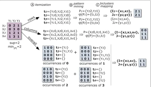
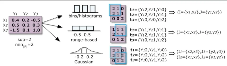
A pattern-based approach to biclustering relies on an itemization step, where the original matrix is transformed into an itemset database, followed by the application of FIM methods under a low support threshold. For real-value matrices, normalization and discretization proce-dures are applied. Then, the discrete value of each cell is concatenated with the respective column index. Each transaction of the target itemset database corresponds to a row with these new values. FIM is applied over the database to mine frequent patterns, which are then used to derive biclusters with constant values on rows. Con-stant values on columns can be mined using the transpose matrix. To find a more constrained type of biclusters, such as constant values overall, each item needs to be mined separately. Figure 2 illustrates how to deliver such types of biclusters using frequent patterns.
Figure 2Discovering biclusters with a constant assumption across rows (a), columns (b) and overall elements (c) using frequent itemset mining.Column identifiers (y1, y2, y3) are combined with the observed values {0,1,2,3}, and FIM applied under a parameterizable support threshold
(θ=2∧ |P| ≥2). Constant values on columns can be mined using the transpose matrix. To find biclusters with constant values overall, each item needs to be separately mined.
and the quality of the output. Two classes of PM-based biclustering approaches can be considered: approaches that directly apply pattern miners over discrete matrices, and approaches that target numeric matrices by customiz-ing the support metric. To our knowledge, BiModule [13], DeBi [10], Bellay’s et al. [30] and GenMiner [15] are the state-of-the-art methods for this first class of PM-based biclustering. BiModule [11,13] allows for a parameter-ized multi-value itemization of the input matrix to dis-cover constant biclusters derived from (closed) frequent patterns using the LCM miner [31]. DeBi [10] derives biclusters from (maximal) frequent patterns mined over binarized matrices using the MAFIA miner [32], and places key post-processing principles to adjust biclusters in order to guarantee their statistical significance. Bellay’s et al. [30] use the Apriori miner with additional princi-ples to evaluate the functional coherency of the discov-ered biclusters against the background noise. GenMiner [15] includes external knowledge within the input matrix to derive biclusters from association rules that relate annotations (external grouping of rows or columns) with computed clusters of rows and columns from (closed) frequent patterns using CLOSE [33]. Although other biclustering approaches seize contributions from these
previous works [34,35], we do not refer to them as PM-based appproaches if the core mining task does not rely on FIM.
The itemization step is optional for the second class of methods [36]. To our knowledge, RAP [14], RCB dis-covery [36] and ET-bicluster [37] are the state-of-the-art methods in this context. RAP [14] plugs an adapted range-based metric to mine constant biclusters on rows (or columns), while RCB discovery targets biclusters with constant values overall [36]. ET-bicluster extends the pre-vious approaches to discover noisy biclusters, although an exhaustive enumeration of biclusters is not guaran-teed [37]. Alternative support metrics with dedicated Apriori-based searches have been additionally referred in literature [38-40].
BicPAM: pattern-based biclustering
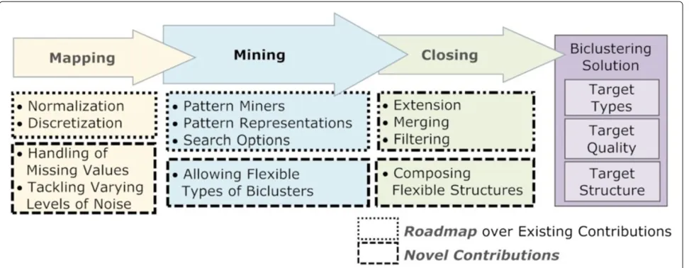
discovery approach, target patterns and search properties. The mapping step consists in the itemization of a real-value matrix into an itemset matrix. This step is driven by normalization and discretization criteria and it may use different principles to handle outlier, numeric or missing elements. Finally, the closing step consists on the post-processing of the output patterns to affect the structure and quality of the target biclusters. Figure 3 clarifies how BicPAM relies on the existing pattern-based contributions and pinpoints the novel principles proposed for each step. The homogeneity criteria can be intentionally defined to search for specific types and structures of biclusters and to affect their quality. The biclustertypedepends on the allowed coherency patterns and on their orientation (row, column or overall), the solutionstructuredepends on the number, size and positioning of biclusters, and, finally, the qualitydefines the allowed noise associated with a single bicluster or with a set of biclusters.
BicPAM is introduced in three following sections. First, we describe the core steps of BicPAM (BicPAM outline). Second, we go further and incorporate new methods to deal with missing values and arbitrary high input levels of noise (Affecting the quality of pattern-based biclusters). Finally, we propose further algorithmic solutions for the discovery of biclusters allowing symmetries and following additive and multiplicative assumptions (Allowing more flexible types of biclusters).
BicPAM outline
This section describes the structural behavior of BicPAM by surveying principles for the mining, mapping and clos-ing steps. These principles are either derived from the
existing pattern-based approaches for biclustering or from advances in the pattern mining field.
Mining step
Understandably, non-constrained settings, where the number of biclusters and their properties is not known apriori, require efficient searches. Pattern mining approaches have been tuned during the last decades to be computationally efficient. Therefore, their adequate use for biclustering is critical and depends essentially on three points described below: 1) the adopted pattern-based approach to biclustering,2)the target pattern representa-tion, and3)the search strategy.
1) Pattern-based Approach
Definition 8.LetLbe a set of ordinal items, a biclus-ter is a sub-matrix(I,J) ⊆ A with its elements aij ∈ L defining a pattern profile. A constant bicluster can follow: i) an overall constant assumption where aij=c and c∈L, ii) a column-based constant assumption where aij = cj and cj∈L, or iii) a row-based constant assumption where aij=ciand ci∈L.
Pattern-based biclustering under a constant assump-tion is the ordinary case. DeBi [10], BiModule [13] or GenMiner [15] only target this type of biclusters. These approaches either rely on Frequent Itemset Mining (FIM) or on association rules, which contrasts with traditional approaches [9,18]. The support threshold defines the min-imum number of rows in a bicluster. In the context of gene expression, a low support is critical since high expression coherency is only observed for small groups of genes and
conditions. Additionally, a post-pruning to the frequent itemsets can be performed in order to filter frequent item-sets below a minimum number of columns and above a maximum number of rows and columns.
From the point of view of an itemized database, the FIM-based biclusters are perfect biclusters, that is, they do not allow value-variations in any of its elements. Contrast-ing, from the point of view of the input real-value matrix, these biclusters can handle noise since two elements with the same item may be numerically distant. The number of items can be used to control the noise-tolerance. However, regardless of the number of items, a common drawback appears when two elements have similar real-values but different items assigned. We refer to this drawback as the items-boundary problem.
BiModule [11] and DeBi [10] are representative FIM-based biclustering approaches. Since their running time is comparable to greedy algorithms, they offer a simplis-tic way to deal with noise and overlapping structures [13]. However, the items-boundary problem can lead to the partitioning of large biclusters into smaller ones (with many being filtered as they no longer satisfy the support criterion).
In order to mine frequent itemsets with different prop-erties, the notion of support of an itemset can be rede-fined. RAP [14] uses a customized anti-monotonic range support merit function. A FIM-based algorithm is used to discover range patterns from real-value matrices without the need for discretization. However, efficiency is strongly penalized.
An additional option to pattern-based biclustering is to derive biclusters from association rules. An associ-ation rule, an implicassoci-ation between two itemsets, can affect the properties of the corresponding bicluster as it constrains the levels of confidence among rows. Option-ally, correlation metrics can be adopted to augment the confidence-support metrics with new interestingness cri-teria. GenMiner [15] uses association rules to compose biclusters. However, the adoption of association rules is only preferred over FIM-based approaches when knowl-edge regarding the dependencies across rows (or columns) is available.
BicPAM uses frequent itemsets as the default pattern-based option to biclustering. Range-pattern-based approaches are only selected for small-to-medium datasets. Finally, in the presence of domain knowledge (such as functional groups of genes or dependencies on conditions), Bic-PAM relies on association rules to compose biclustering solutions.
2) Pattern Representations
The target pattern representation depends essentially on: 1)the selected type and structure of biclusters, and
2) the post-processing needs. Efficiency is not a strong criterion, since only subtle gains are observed for meth-ods that target constrained representations, such as closed and maximal representations.
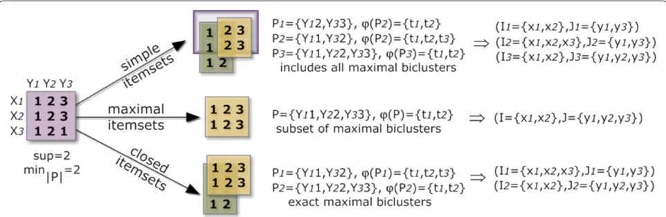
The use of all frequent itemsets leads to biclustering solutions with a high number of (potentially redundant) biclusters (if contained by another bicluster), which can degrade the performance of the mining and closing steps. Contrasting, the use of maximal itemsets leads to biclus-ters with the columns’ size maximized. Maximal itemsets for biclustering are adopted in DeBi [10]. Such flattened biclusters are particularly interesting when there is an extension step to be performed to include new rows for the discovered biclusters. However, since both vertical and smaller biclusters are avoided, maximal-based biclusters lead to incomplete solutions as they are just a subset of all valid biclusters.
Finally, by using closed itemsets, we allow for over-lapping biclusters only if a reduction on the number of columns from a specific bicluster results in a higher num-ber of rows. Note that to obtain maximal biclusters – biclusters that cannot be extended without the need of removing rows and columns – closed patterns need to be used instead of maximal patterns. FIM-based BiModule [13] and rule-based GenMiner [15] use closed itemsets as the means to compose biclusters.
BicPAM uses frequent closed patterns as the default representation. The set of all and maximal frequent pat-terns are also made available in BicPAM. An illustration on how different types of pattern representations lead to structurally different biclustering solutions is provided in Figure 4.
3) Search Strategies
The definition of the search setting depends essentially on:1)the fit of the search with the target biclustering task, and2)the chosen implementation.
Figure 4Comparison of biclustering solutions using frequent itemsets, maximal frequent itemsets and closed frequent itemsets.
exponentially degrades with an increasing number of items.
Several algorithms were developed for each of these search strategies. However, their properties should be carefully assessed, as their nature is most of the times optimized towards specific sets of datasets. In the DeBi [10], BiModule [11] and GenMiner [15] biclustering tasks, Mafia [32], LCM [31] and CLOSE [33] are, respectively, the algorithmic choices.
BicPAM makes available a variant of FP-Growth that traces the set of transactions per frequent pattern [44] (default option), Charm [45], AprioriTID [41] and Eclat [43]. Finally, Carpenter [46] and Cobbler [47] are addi-tional algorithmic choices in BicPAM to compose biclus-ters with a large number of columns and for large-scale datasets.
Mapping step
Normalizationtechniques are often required to enhance differences across rows and/or columns. Alternative methods have been reported [34,48]. BicPAM allows the normalization criteria to be applied in the context of a row, a column or the overall matrix. Additionally, it makes available a zero-mean value to allow for symmetries and to provide a simple setting for the approximation of probabilistic distributions. In the presence of missing and outlier elements, a masking bitmap can be used in order to exclude them from the computation of the mean and dispersion metrics.
Discretization is an additional key step for pattern-based methods relying on itemset databases. Although discretization may imply loss of information, it allevi-ates the noise dilemma [26] and it is the cost to pay for exhaustive searches. BicPAM makes available multiple discretization options with key implications on the tar-get solution. Two axes are considered:1)the number of items (also referred as symbols) and2)the target method to map the normalized real-value matrix into a itemset
database. Increasing the number of items is commonly used to improve quality, but it reduces the average size of biclusters and the number of biclusters produced. A sensi-tivity analysis on the impact of choosing different number of items was performed in Bidens [34] and BiModule [13]. The three discretization methods made available in Bic-PAM are illustrated in Figure 5. The use of fixed ranges (potentially equal sized intervals between the observed maximum and minimum) is the simplest discretization option, but commonly leads to an accentuated weak dis-tribution of items and is prone to the items-boundary problem. The first problem can be corrected using a percentage-based method for the depth partitioning of items that leads to intervals containing approximately the same number of items. Bidens [34] uses this equal-depth partitioning method over a data context where outliers are temporarily removed. Finally, alternative distributions can be used to combine the properties of the previous solutions, such as the setting proposed in Nordi [15]. By finding multiple suitable curves (for each row or col-umn) or one suitable overall curve for approximating the matrix, we can either use threshold methods or directly compute the statistical cutoff points to create equally-distributed areas. In the illustration, a Gaussian distribu-tion is selected to minimize the loss of potentially relevant biclusters.
Closing step
Figure 5Impact of discretization options available in BicPAM.
(commonly connected with overlapping biclusters), Bic-PAM enables the use of criteria structured according to three stages:1)extension,2)merging and3)filtering.
1) Extension Options
Three optional and non-exclusive strategies can be used to extend the discovered biclusters such that the result-ing solution still satisfies some pre-defined homogeneity criteria. First strategy consists on the use of statistical tests to include rows or columns over each bicluster as proposed in DeBi [10]. Second strategy relies on tradi-tional approaches and on their merit functions for further extensions as long as the solution satisfies either the intra-or inter-bicluster homogeneity criteria. Finally, we pro-pose a third strategy that uses patterns discovered under more relaxed criteria (such as lower support-confidence thresholds) to guide the extension step. When consider-ing lower supports, new columns and rows can be added to the original frequent patterns. Similarly, more relaxed association rules, with less restrictive ways to group the antecedent-consequent, can be used to guide the exten-sion step. The use of simple thresholds, of statistical tests or of merit functions to verify if the bicluster is valid can either be computed using the discretized matrix (item matchings) or, more interestingly, the distances from the original real-value matrix.
2) Merging Options
Merging operations serve two goals: noise allowance and overall biclustering structure manipulation. The first goal is driven by the observation that when two biclusters share a significant area it is probable that their merging composes a larger bicluster still respecting some homo-geneity criteria. Commonly, such decomposition is related with the items-boundary problem or with a missing value. The simplest criterion to allow the merging is either to rely on the overlapping area (as a percentage of the smaller bicluster), to compute the overall noisy percentage after the merging, or to use advanced homogeneity criteria
(potentially relying on the real-values provided by the input matrix). State-of-the-art procedures to efficiently merge pattern-based biclusters include [49,50].
3) Filtering Options
Filtering is possible at two levels:1)at the bicluster level, and 2)at the row-column level. The first type of filter-ing is required to remove duplicates and biclusters that are contained in larger biclusters. The existence of biclus-ters included in larger biclusbiclus-ters is a necessary result of the extension-merging options and it is a common prob-lem when adopting mining approaches that do not rely on condensed pattern representations. Both DeBi [10] and BiModule [13] provide alternative heuristics to efficiently perform this type of filtering.
The second type of filtering can be used to exclude rows or columns from a particular bicluster in order to inten-sify its homogeneity. This is usually the case when a low number of items is considered, leading to highly noise-tolerant biclusters. For this purpose, similarly to extension options, we can rely on three strategies: 1) use statisti-cal tests on each row and column of a particular bicluster in order to identify removals,2)rely on existing greedy-iterative approaches and maximize their merit functions (which can imply a reduction on the size of biclusters), and 3)discover patterns under more restrictive conditions (as higher support and confidence thresholds).
Affecting the quality of pattern-based biclusters
BicPAM options with impact on the solution quality include:
– Mining step options, including the approach, the support-confidence thresholds, and the pattern representations;
– Mapping step options, including the number of items and the normalization-discretization techniques; – Closing step options, including the selected
their criteria thresholds (percentage of noise, overlapping degree, statistical significance levels).
Below, we describe new strategies that BicPAM makes available to handle varying levels of missing values and input noise, and to compose multiple structures of biclusters.
Handling missing values
The input matrices can have an arbitrary high number of missing values, as it is common in GE matrices. A non-treated missing value may result in the loss of a critical row and of a column across one or more biclusters. Three different strategies can be applied to treat missing values: 1)removal,2)replacement, and3)handling as a special value. The simplest method is to remove the contain-ing row or column (usually the dimension with smaller size).
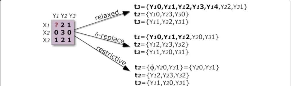
Many hole-replacing methods have been proposed [51-53], alleviating the referred problem, although intro-ducing additional noise that can significantly decrease the homogeneity of the output biclusters. For this reason, we propose the use of an additional item that is specially han-dled according to a level of relaxation hanhan-dled by the user, as illustrated in Figure 6. The lowest constrained setting (relaxed) replaces the missing item by all other adopted items, which again results in transactions with varying size. The medium constrained setting (δ-replace) con-siders multiple items around its value-estimation. If the difference between the estimated value and the centroid-value of a discretization range is less thanδ, then the item assigned to the range is added. In BicPAM, the default imputation method is based on the mean values for the four nearest neighbor rows. BicPAM defaultδ distances guarantee a lower bound of two items and an upper bound of three items. The highest constrained setting (restrictive) removes missing items.
Handling varying levels of noise
A key direction to pattern-based biclustering is to con-sider multiple levels of noise by following one of the three strategies illustrated in Figure 7. First strategy (reduced number of items) hierarchically joins contiguous items (items are viewed as being ordinal and no longer nominal) to mine biclusters over matrices with different number of items. Optimizations to this strategy can be made by col-lapsing items only for some critical areas of the matrix where the presence of biclusters is scarcer. Understand-ably, the level of noise should be maintained by each bicluster, so that closing steps can be adapted in respect to the quality of the target bicluster.Secondstrategy (relaxed-to-restricted extensions) considers varying levels of noise only after the mining. For instance, the merging of con-stant biclusters can follow a statistical test sensitive to the closeness of different items (heuristics based on overlap-ping rows-and-columns should also be considered).Third strategy (multiple items) associates one or more items to each element based on a parameterized threshold. Dif-ferent criteria can be defined to assign a varying number of items per element aij. Each element can be mapped into two-to-three items based on the distance to their centroids leading to transactions with multiple sizes.
Producing alternative biclustering structures
Since the number of biclusters is neither fixed nor depends on the satisfaction of local coverage criterion, pattern-based approaches provide a heightened flexibil-ity for the composition of different biclustering structures. A pattern-based solution is non-exhaustive, non-exclusive and allows overlaps. The task of composing different structures has been poorly addressed in literature, and rather seen as the byproduct of biclustering methods [1]. Below, we introduce a set of principles to compose multiple structures made available in BicPAM.
For an exhaustive structure (either overall, across rows or across columns), biclusters can be incrementally
Figure 7Strategies to deal with noise-relaxations.
merged following, for instance, an hierarchical criteria based on the proximity and the area of biclusters, until all the matrix is covered. If the goal is anexclusivestructure (either overall, across rows or across columns), a simple strategy is to merge biclusters in order to reduce overlap-ping across one or both dimensions and, additionally, to filter biclusters that share rows or columns following an relevance criterion (as size or noise level) until exclusiv-ity is guaranteed. Closing options can be specifically used to produce other alternative structures with sharp usabil-ity (no need to change the core tasks of pattern-based approaches).
Allowing more flexible types of biclusters
Below, we extend BicPAM to consider more flexible expression patterns: additive, multiplicative and symmet-ric coherency.
Coherency under additive-multiplicative assumption
Definition 9.A bicluster(I,J)follows an additive model if aij=c+αi+βj+ηij, where c is the typical value within the bicluster,αi is the adjustment for row i ∈ I,βj is the adjustment for column j∈J andηijis the noise associated with the element. A bicluster(I,J)follows a multiplicative model if aij=c×αi×βj+ηij, which is equivalent to the additive model when c=logc,αi=logαiandβj=logβj.
We propose two pattern-based strategies for the discov-ery of biclusters with non-constant models of coherency. The first strategy is to use local normalization procedures to correct row- or column-based differences and then to map the task into the search for constant biclusters.
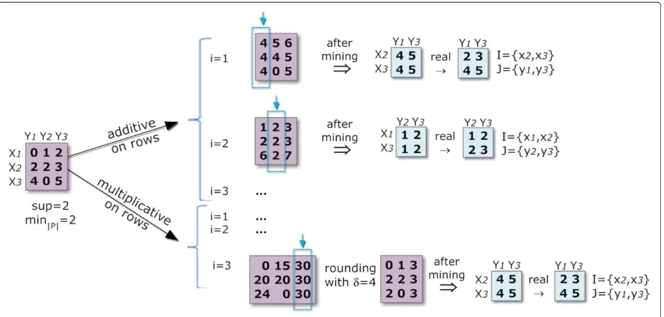
The second strategy, the default BicPAM option, is to iteratively perform alignments on each column (or row). This guarantees that all the alignments needed to compose these biclusters are considered. Therefore, the
selected pattern miner is applied eitherm (orn) times, leading to a higher computational complexity. Figure 8 illustrates this strategy.
An additive alignment over a target column yj can be computed by adding for each element on the row xi the difference between the maximum of the column and the discretized valuemax(yj)−aij. A multiplicative alignment over a target columnyj can be computed by adding, for each element on the rowxi, the least common multiple between the maximum of the column and the discretized value lcm(max(yj),aij). The resulting number of items under an additive assumption is in the worst case the double of the number of items initially considered. The number of final items under a multiplicative model is the size of thelcmcombinations across the initial items. As illustrated in Figure 8, a distance-based δ-error can be considered to gather close items in the multiplicative model due to the lower probability of finding coherent biclusters as a consequence of the resulting large number of items.
Coherency under symmetrical assumption
A critical, but less studied, type of biclusters is biclusters with coherent values under symmetrical assumption, also referred as biclusters with sign-changes in literature [1]. Two rows or columns from a bicluster allowing symme-tries may have similar absolute values differing in sign. Such biclusters can simultaneously capture activation and repression mechanisms within a biological process.
Figure 8Pattern-based discovery of biclusters under additive and multiplicative assumptions.
symmetry factor and aij ∈ Ris an element of a bicluster with coherent values.
For the purpose of finding biclusters with symmetries, the normalization should satisfy the zero-mean criterion. Additionally, if the number of considered items is odd, there is one item being its own symmetric that must be specially handled.
One option is to align the sign of activity of each row (or column) in order to guarantee consistency of signals for a target column (or row). The top example in Figure 9 illus-trates this strategy. An iterative mapping for every column (or row) is possible, although additional efficiency can be
achieved by stopping the search when all the sign combi-nations have been achieved. Nevertheless, the worst case requires the application of a pattern minerm times (or n times). Note that filtering is a critical step needed to remove potential duplicates resulting from repetitions of alignments for subsets of rows (or columns).
The combination of this strategy with the search for biclusters under an additive or multiplicative model can be expensive (m×mtimes iterations). Therefore, BicPAM makes available an additional option to combine the use of the sign and of the additive or multiplicative adjustments together for every column (or row). This model (combined sign and coherent model) is not equivalent to the previous
model (sign plus coherent model), since it assumes that additions or multiplications are not absolute but depend on the activity slope sign. Here, the value adjustment of a particular element is also affected by the sign, which can lead to an additional number of items. This strategy is illustrated in the bottom example of Figure 9.
Algorithm 1: BicPAM core steps
Input: matrix, coherency, orientation, nrItems, patternMiner, patternRep, normalizer, discretizer, missingsHandler, noiseHandler, extender, merger, filter, stopCriteria/*default arguments when absent*/
1 mainbegin
2 itemizedData←runMappingStep(matrix, nrItems, normalizer,
discretizer, missingsHandler, noiseHandler, orientation);
3 biclusters←runMiningStep(coherency, patternMiner,
itemizedData, patternRep, stopCriteria, nrItems, orientation);
4 returnrunClosingStep(biclusters, extender, merger, filter); 5 runMappingStepbegin
6 mask←getMissingsOutliersMask(matrix);
7 discData←discretize(matrix, nrItems, normalizer, discretizer,
mask);
8 ifisColumn(orientation)thendiscData←transpose(discData)
9 treatedData←appHandlers(discData, missingsHandler,
noiseHandler);
10 returncreateTransactions(treatedData); 11 runMiningStepbegin
12 ifisConstant(coherency)thenfreqItemsets←
runFIM(patternMiner, itemizedData, patternRep, stopCriteria)
13 elsefreqItemsets←runIterativeFIM(coherency, patternMiner, itemizedData, patternRep, stopCriteria)
14 // recover columns and rows from frequent itemsets
15 returngetBiclusters(freqItemsets, nrItems, orientation);
16 runClosingStepbegin
17 biclusters←merge(biclusters, merger);
18 biclusters←filterBiclusters(biclusters, filter);
19 biclusters←extend(biclusters, extender);
20 returnincreaseConsistency(biclusters, filter);
21 runIterativeFIMbegin 22 factors← ∅;
23 freqItemsets← ∅;
24 foreachcolumn j in itemizedDatado
25 // different for additive, multiplicative and symmetric coherencies
26 colAdjusts←computeFactor(itemizedData[·][j],coherency);
27 ifcolAdjusts∈factorsthencontinue
28 elsefactors←factors∪colAdjusts
29 alignedData←alignDataByRows(colAdjusts,itemizedData);
30 freqItemsets←freqItemsets∪runFIM(patternMiner, alignedData, patternRep, stopCriteria);
31 // simple combinatorial calculus to prune the search
32 ifallCombinations(factors)thenbreak
33 return freqItemsets;
34 runFIMbegin
35 ifestimateLimits(stopCriteria)then
36 // simple statistical calculus based on the frequency of items
37 (minRows,minColumns)←
findLowerLimitsExpectations(data);
38 freqItemsets←FIM(patternMiner, minRows, minColumns, data, patternRep);
39 else
40 minSupport←0.5; 41 freqItemsets← ∅;
42 whileminAreaPercentageAchieved(freqItemsets,10%)do 43 freqItemsets←FIM(patternMiner, minSupport, data,
patternRep);
44 minSupport←minSupport×0.8; 45 return freqItemsets;
BicPAM algorithm and complexity analysis
The algorithmic basis of BicPAM is described in Algorithm 1. Although BicPAM follows a plug-and-play style, default and data-driven parameterizations are made available. In particular,lines 40-44and37describe BicPAM behavior in the absence of user-driven parame-terizations. This is performed by either relying on esti-mation procedures or on convergence criteria based on thresholds such as the relative area covered by biclusters or the minimum number of biclusters.
The computational complexity of BicPAM is bounded by the pattern mining task and computation of similarities among biclusters. For this analysis, we cover major com-putational bottlenecks related with each one of the three major steps of BicPAM. Within themappingstep: outlier detection, normalization, discretization, and noise correc-tion procedures (such as the assignment of multiple items) are linear on the size of the matrix,(nm). The optional distribution fitting tests and parameter estimations to dynamically select an adequate discretization procedure are also(nm). These tests and estimations rely on the calculation of approximated statistical ratios [54]. Han-dling missings by removing the respective element or by replacing them by a special dedicated item is also(nm). However, when an imputation method is selected, the complexity is upper bounded by(hnm), wherehis the number of missing values. In BicPAM implementation, the nearest neighbor rows and columns are computed for the estimation of each missing value.
The cost of the mining step depends on two factors: the complexity of the pattern miner and the need for iterations for the discovery of non-constant profiles. The cost of the pattern mining task depends essentially on: the number and size of transactions (γnm, where γ ≥ 1 captures the increase in size related with noise and missings handlers), the frequency distribution of items ({L×Y} →N), the minimum supportθ, the pattern rep-resentation and the selected mining procedure. A detailed analysis of this complexity has been attempted in liter-ature [55] and it is out of the scope of this paper. The reader should also keep in mind that there has been proposals to guarantee the scalability of pattern min-ers recurring to partitioning and approximation meth-ods [12]. Let(℘ (γ,n,m,|L|,θ)), or simply(℘), to be the complexity of a pattern mining task. When there is the need for the iterative application of the core min-ing procedure, the overall search is bounded by (d ×
℘), where d = minn2,m when allowing symme-tries,d = min|Ln|,mwhen allowing shifts, andd =
minlcmn ,mwhen allowing scaling factors.
and the complexity of extending and reducing biclus-ters. To compute similarities a tree structure is created where each node represents a gene and each leaf corre-sponds to a bicluster. Only biclusters sharing a branch over a threshold based on the input overlapping degree are candidates for merging and filtering. Filtering a bicluster results in the removal of its leaf and dedicated nodes. Merging two biclusters results on the combination of the target branches. These tasks have an average complexity of kk/2¯r¯s
, where k is the number of biclusters and ¯
r¯stheir average size. Extending biclusters relies on quick tests based on the coherency of each new column or row and therefore the complexity of this task is respectively (k¯rm)or(kn¯s), wherekis the number of biclusters after merging and filtering. Removing rows or columns from biclusters is(kr¯¯s).
In this context, the complexity of BicPAM is bounded
by
hnm+d℘+kk/2r¯¯s+k(¯rm+n¯s)
, which for set-tings resulting in a large number of biclusters after the mining step (kk) is approximately
d℘+kk/2r¯s¯
.
Results
In this section, we present an extensive experimental eval-uation showing that BicPAM is effective and computa-tionally efficient. BicPAM was implemented in Java (JVM version 1.6.0-24). The following experiments were run in an Intel Core i3 1.80 GHz with 6 GB of RAM.
The results were collected and analyzed in four steps. Section “Comparison of biclustering approaches in syn-thetic data” compares the performance of BicPAM against state-of-the-art biclustering approaches. In Section “Per-formance analysis in synthetic data”, BicPAM’s behavior is extensively assessed in synthetic datasets with vary-ing size, noise, sparsity and background distributions. The biological relevance of BicPAM’s results is analyzed in Section “Results in real data”. Finally, Section “Compar-ison of pattern-based biclustering approaches” goes fur-ther on comparing BicPAM and its pattern-based peers. Below, we describe the evaluation metrics and data set-tings used.
Evaluation metrics. Biclustering solutions have been assessed using multiple evaluation criteria. In the presence of hidden/planted biclusters, H = {H1, ..Hg}, clustering metricsa, match scores [2,58] and relative non-intersecting area (RNAI) [59,60] have been used. Match scores (MS) [58] assess the similarity of solutions based on the Jaccard index. MS(B,H) defines the extent to what found biclusters match with hidden biclusters, while MS(H,B) reflects how well hidden biclusters are recov-ered (1). RNIA [59] measures the overlap area between the hidden and found biclusters. To distinguish if several or few of the found biclusters cover a hidden bicluster, clus-tering error(CE) [60] is a critical extension. To take into
account the number of biclusters in both sets, Hochreiter et al. [2] introduced a consensus score by computing sim-ilarities between all pairs of biclusters (2). We refer to this metric as FABIA Consensus (FC). LetS1andS2be, respec-tively, the larger and smaller set of biclusters from{B,H}, andMPbe the assigned pairs using the Munkres method based on overlapping areas [61], MC and FC are defined as:
MS(B,H)= 1
|B|(I1,J1)∈Bmax(I2,J2)∈H |I1∩I2| |I1∪I2|
, (1)
FC(B,H)= 1
|S1|((I1,J1)∈S1,(I2,J2)∈S2)∈MP
× |I1∩I2|×|J1∩J2|
|I1|×|J1|+|I2|×|J2|−|I1∩I2|×|J1∩J2|.
(2)
In the absence of hidden biclusters, merit functions can be used as long as they are not biased towards the merit criteria used within the approaches under compari-son. Examples include the commonly used mean squared residue (MSR) [62] and its extension [16], or the Pearson’s correlation coefficent [59] sensitive to shifting-scaling properties. Finally, domain-specific evaluations can be used by computing statistical enrichmentp-values in bio-logical contexts [10,63].
Data settings. Gene expression data and two sets of synthetic datasets were used to evaluate BicPAM perfor-mance. The first set corresponds to the datasets generated by Hochreiter et al. [2]. These datasets simulate specific characteristics of gene expression data, such as heavy tail properties, using three settings: multiplicative models and additive models under signals according to N±2, 0.52 andN±4, 0.52distributions [64]. Each setting has 100 datasets with 1000 genes, 100 conditions and 10 planted biclusters.
A second set of synthetic datasets with varying size and planted biclusters with varying degrees of expression was generated in the context of this work [65] (settings described in Table 1). We varied the size of the matrices up to 4.000 rows and 400 columns, maintaining the pro-portion between rows and columns commonly observed in gene expression data. The number and shape of the planted biclusters were also varied. The properties of the generated matrices were carefully chosen in order to follow properties from similar studies [10,13].
Table 1 Properties of the generated set of synthetic datasets
Matrix size (rows×cols) 100×30 500×60 1000×100 2000×200 4000×400
Nr. of hidden biclusters 3 5 10 15 20
Nr. columns in biclusters [5,7] [6,8] [6,10] [6,14] [6,20]
Nr. rows in biclusters [10,20] [15,30] [20,40] [40,70] [60,100]
Area of biclusters 9.0% 2.6% 2.4% 2.1% 1.3%
noise factor is up to ±15% of the range of values (e.g. aij←aijU(−1.5, 1.5)when 10 items are available).
For each of these settings we instantiated 40 matrices: 20 matrices with background values following a Uniform distribution, U(1,|L|), and 20 matrices with background values generated according to a Gaussian distribution, N|L2|,|L6|. The performance of BicPAM is an average across these 40 matrices.
Comparison of biclustering approaches in synthetic data We selected five state-of-the-art approaches able to dis-cover biclusters under additive-multiplicative assump-tions: FABIA with sparse prior option [2], Bexpa [66], ISA [67], Plaid [6] and OPSM [19]. Additionally, we considered CC [62], Samba [9], xMotifs [18], and three pattern-based biclustering approaches: BiModule [13], DeBi [10] and RAP [14]. Although the last six biclustering approaches use more simplistic homogeneity criteria, their inclusion is critical to study the biological significance of BicPAM’s solutions and to test BicPAM’s performance improve-ments when considering biclusters with constant models. We used the following software to run these meth-ods: R packages fabia [68] and biclust [69], BicAT [70], (Evo-)Bexpa[66] andExpander[71]. The specified num-ber of biclusters for FABIA (with and without sparse equation), Bexpa, CC and ISA (number of starting points) was the number of hidden biclusters plus 10%:|H| ×1.1.
Note that this required specification can be used to guide the search space exploration against other biclustering approaches and optimistically bias FABIA consensus (FC) levels. The default number of iterations for OPSM was varied from 10 to 200 iterations. The remaining meth-ods were executed with default parameterizations. For this comparison, BicPAM was parameterized with closed pat-terns discovered using discretization methods with three distinct sets of items (|| ∈ {3, 5, 7}), under a simple merging option (70% overlap) and filtering of biclusters based on an overlapping area over 30% against a larger bicluster. Additionally, two items were assigned to values near item-boundaries, leading to an increase in the size of transactions of 8-11%. The support threshold was incre-mentally decreased 10% and stopped when the discovered biclusters covered a minimum area of the input matrix (>5%×|X| × |Y|).
The ability of these approaches to retrieve the hidden biclusters using FABIA data settings is synthesized in Figure 10. FC(B,H)was measured across the 100 matrices generated for each setting. BicPAM is the best performer for biclusters following additive models with different signal properties (Wilcoxon-test at 0.01%) and, together with FABIA, the best option for multiplicative models. The exhaustive nature of BicPAM searches and the abil-ity to rely on multiple discretization levels without risk of introducing noise (by assignment multiple items for val-ues near ranges-boundaries) support these observations.
Figure 11Match scores across biclustering approaches using FABIA datasets.
FABIA is a competitive non-exhaustive alternative, sensi-tive to the planted noise. Nevertheless, it requires prior knowledge regarding the number of biclusters. Since ISA is tunned to discover biclusters with gradual changes on values, its scoring schema to find modules with self-consistency is not well suited to discover biclusters mod-eled by additive signals. Plaid is able to locally identify additive factors. Understandably, the set of approaches not able to discover biclusters with scaling and shift-ing factors is considerably less effective. The FC levels of OPSM are strongly penalized since OPSM outputs a large number of biclusters with varying sizes (includ-ing biclusters with either small number of genes or conditions).
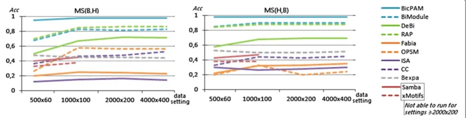
A comparison of match score levels across bicluster-ing approaches when usbicluster-ing the FABIA generated datasets is provided in Figure 11. Results confirm the superior performance of BicPAM both in terms of the MS(B,H) score (correctness) and MS(H,B) score (completeness). BicPAM is able to exhaustively mine the solution space and combine multi-level discretization thresholds. The average efficiency levels of BicPAM show its ability to perform exhaustive searches in useful time for
compu-tationally complex settings. FABIA is the most efficient approach.
Figures 12 and 13 assess the ability of the analyzed biclustering approaches to discover planted biclusters with different coherency criteria (using an alphabet with 10 levels of expression) and varying the number of rows and columns (planted according to an Uniform distribu-tion). Figure 12 shows that BicPAM’s performance (in the absence of extensions to discover non-constant biclusters) is superior against the three peer pattern-based meth-ods. Figure 13 captures relevant changes in performance when considering additive and multiplicative coheren-cies. In order to promote the readability of these charts, we excluded the performance of the approaches not pre-pared to discover biclusters under these assumptions. Results confirm the superior performance of BicPAM in terms of MS(B,H), that is, the majority of the discov-ered biclusters are well described by the hidden biclusters (correctness), and MS(H,B), that is, the majority of the hidden biclusters can be mapped into a discovered biclus-ter (completeness). Although FABIA is the second choice for non-constant coherency, it is not prepared to deal with overlaps and it accommodates high levels of noise since
Figure 13Match scores of biclustering approaches using datasets with non-constant models.
it is not prepared to differentiate all of the 10 levels of expression, resulting in biclusters with a larger number of false positive genes.
Finally, Figure 14 shows that, although all approaches are scalable for medium-sized matrices, efficiency dete-rioration is faster for OPSM, BicPAM and CC. The effi-ciency of peer pattern-based approaches is slightly worse than that of BicPAM as they do not seize the benefits of FP-growth searches.
Performance analysis in synthetic data
In this section we study the efficiency limits of BicPAM. Then we assess the ability of BicPAM to discover differ-ent types of biclusters for data with varying regularities. Finally, we go further on understanding the impact of using different strategies related with the mining, map-ping and closing steps.
Efficiency limits
To show the boundaries on BicPAM efficiency we consid-ered matrices with 10.000 rows (magnitude of the human genome). The results are provided in Figure 15. We var-ied the number of conditions, the number of items (|L| ∈ {5, 7}) and the underlying coherency assumptions for this assessment. We consider the default merging procedure for the closing step. We planted 15 biclusters to occupy 2% of the area of the generated matrices and used Charm algorithm [45], an efficient pattern miner to deliver closed
patterns (maximal biclusters). Generally, we observe that BicPAM is able to discover constant biclusters for matri-ces up to 10.000×350 and additive/multiplicative biclus-ters for matrices up to 10.000 × 200. Understandably the number of items has strong impact in efficiency as it defines the density of the correspondent itemset database and, therefore, the complexity of the mining step. Note, additionally, that the extensively studied scalabil-ity principles based on extensions over pattern mining methods – parallelization, distribution, streaming and error-bounding principles [12] – can be easily included in the mining step of BicPAM to guarantee its scalability over harder data settings.
Recovery of (non-)constant biclusters
Although BicPAM relies on exhaustive searches, its per-formance highly depends on the ability to deal with noise, discretization errors and coherency assumptions. Figure 16 shows BicPAM’s performance with a parameter-izable number of items for the datasets generated under a constant assumption. FC levels are attractive, although they are penalized by the exclusion of rows due to the planted noise, allowed overlapping among planted biclus-ters together with the fact that the number of discovered biclusters is usually higher than the number of planted biclusters.
A smaller number of items turns the matrix denser, decreasing the efficiency bounds of BicPAM. Using a similar experimental setting, Figure 17 illustrates the
Figure 15Efficiency bounds of BicPAM for 10000 rows (magnitude of the human genome).
performance of BicPAM for datasets with planted biclus-ters with an additive assumption. Although the observed FC scores are high, they are worse than for constant datasets due to the higher probability of background values to form a non-planted additive bicluster. Inter-estingly, although a na?ve search for additive biclus-ters would cost as much as |Y| times as the search for constant biclusters, the considered pruning fosters efficiency.
Finally, Figure 18 illustrates BicPAM’s performance under a multiplicative assumption. Contrasting with the previous analysis, FC levels decrease for the larger matri-ces as the multiplicative factor is more prone to local mismatchings. This problem can, however, be corrected through closing options. Similarly to the search for additive biclusters, BicPAM seizes efficiency gains by pruning the search space. Additionally, the multiplica-tive assumption is structurally more efficient than its additive peer since the number of spurious biclusters is considerably low due to the broader range of items observed within each iteration, which leads to sparser matrices.
To complement previous analysis, Figure 19 provides BicPAM’s MS(B,H) levels for different levels of expres-sion. The observed MS levels are higher than FC lev-els due to the absence of penalizations of outputting more biclusters than the number of planted biclusters. In particular, MS levels for medium- to-large datasets are, respectively, above 95%, 91% and 87% for constant, additive and multiplicative.
A detailed look of BicPAM’s performance, when con-sidering 7 items and default noise handling, merging and filtering options, is provided in Table 2. The results are organized according to bicluster type, matrix size (and structure of planted biclusters) and underlying distribu-tion of background values. The slightly worse perfor-mance when the input values are generated by a Gaussian distribution is not related with the increased probability of background values to form non-planted biclusters (since values are properly discretized), but with the increased difficulty of modeling the planted biclusters with Uniform
values. We found MS(B,H) to be lower than MS(H,B) since the exhaustive nature of BicPAM leads to at least one found bicluster with a direct correspondence to each hidden bicluster.
Mining options
Figure 20 illustrates the impact of the algorithmic choice in the efficiency of BicPAM. The three main paradigms for frequent itemset mining (Apriori, FPGrowth, and vertical-based Eclat) were tested vertical-based on implementations from SPMF [72] software. These methods were extended in order to be able to deliver the transaction set support-ing each frequent itemset. For this assessment we used a discretization step with 10 items and constant planted biclusters based on all frequent patterns. The results were collected for the 1000 × 100 generated dataset setting. FPGrowth and Eclat are the most competitive choices when dealing with very small support thresh-olds. In particular, FPGrowth is the best performer for the setting used for supports near and below 1%. Finally, Apriori is the best option for medium-to-large support levels.
The impact of choosing alternative pattern representa-tions (simple, closed, maximal) in efficiency and MS levels is presented in Figure 21. For this assessment we used three distinct methods: FPGrowth [42] to output simple patterns, Charm [45] to output closed patterns (maximal biclusters) and CharmMFI [45] to output maximal pat-terns. Similarly, we considered the 1000×100 setting and 10 items.
Figure 16Performance of BicPAM under a constant assumption.
Figure 17Performance of BicPAM under an additive assumption.
Figure 18Performance of BicPAM under a multiplicative assumption.
Table 2 FC and MS levels of BicPAM in different settings (mean and variance from 20 datasets)
100×30 500×60 1000×100 2000×200
Metric Coherency Normal Uniform Normal Uniform Normal Uniform Normal Uniform
FC
Constant 0.862±0.017 0.930±0.014 0.884±0.018 0.956±0.007 0.909±0.017 0.949±0.006 0.907±0.014 0.948±0.011
Additive 0.782±0.021 0.831±0.008 0.834±0.014 0.888±0.007 0.845±0.018 0.897±0.007 0.827±0.015 0.887±0.006
Multiplicative 0.762±0.028 0.794±0.013 0.790±0.019 0.825±0.014 0.785±0.020 0.840±0.011 0.767±0.020 0.819±0.015
MS(B,H)
Constant 0.923±0.018 0.974±0.007 0.931±0.012 0.968±0.005 0.935±0.010 0.984±0.005 0.944±0.011 0.987±0.008
Additive 0.895±0.017 0.945±0.006 0.925±0.012 0.963±0.003 0.913±0.008 0.981±0.007 0.917±0.011 0.974±0.006
Multiplicative 0.902±0.019 0.958±0.014 0.906±0.015 0.953±0.009 0.910±0.015 0.941±0.008 0.886±0.019 0.948±0.010
MS(H,B)
Constant 0.956±0.013 0.984±0.006 0.960±0.007 0.981±0.004 0.961±0.004 0.996±0.002 0.957±0.009 0.993±0.002
Additive 0.955±0.012 0.997±0.001 0.959±0.006 0.997±0.002 0.955±0.004 0.995±0.002 0.957±0.007 0.995±0.003
Multiplicative 0.937±0.015 0.966±0.008 0.924±0.012 0.968±0.008 0.923±0.010 0.963±0.009 0.927±0.013 0.974±0.007
contained in larger planted biclusters, even when the dis-covered biclusters have a heightened homogeneity. Third, the search for closed and maximal patterns is slightly more efficient than the search for simple patterns as a result of additional pruning procedures. These observations sup-port the use of closed patterns. Furthermore, they corre-spond to maximal biclusters, which are in general the aim of effective biclustering algorithms [1,13,73].
Mapping options
In order to assess the impact of the proposed mapping strategies to handle missing values (Figure 6), we ran-domly removed a varying number of elements from the generated matrices for the 1000×100 setting. Figure 22 illustrates how the performance of BicPAM (using Charm and 10-item discretization) varies with a percentage of missings ranging from 0 to 10% (that is, from 0 to 10.000 elements). Note that 10% is already considered a very crit-ical number of missings that may compromise the ability to retrieve the true biclusters. We observe that this prob-lem can be mitigated recurring to the proposed BicPAM missing handlers.
When analyzing the results in Figure 22, three obser-vations can be retrieved. First,MS(B,H)under the base-line strategy (remove the missings) significantly decreases from 97% to near 70% when the percentage of missings reaches 10%. Although this solution is easily implemented
in BicPAM (removing an element from respective trans-actions), the majority of existing biclustering algorithms only allow for removals on the columns or the rows where a missing occurs (impracticable even in the presence of a few missings as illustrated). Second, the ability to retrieve the planted biclusters increases when considering the nearest 2-3 values against the strategies that consider the closest value only or all the possible values (relaxed strat-egy). This is justified by two factors:1)when estimating more than one value for a missing, there is an increased chance to recover the original value and, therefore, of not damaging a planted bicluster;2)when considering all the possible values for a missing, there is an increased amount of noise that is added and can lead to the emergence of false biclusters. Third, although inserting multiple values to replace a missing is an attractive option in terms of accuracy, its efficiency is penalized as the itemized matrix becomes denser (consistent with the number of discov-ered biclusters). Still, when considering only the closest 2-3 values, scalability is maintained for levels of noise up to 10%.
Closing options
We planted additional levels of noise to evaluate the closing options. This was performed by changing the values of specific elements by a randomly distant value (distance>25% of the domain range). The percentage of
Figure 21Impact of choosing alternative pattern representations over the 1000×100 data setting.
noisy elements was varied from 0 to 10%. We used the 1000×100 setting, Charm and a total of 10 items.
Figure 23 describes the impact of alternative strategies toextendbiclusters. When no noise is planted, merging-based strategies are able to achieve slightly higher match-ing scores since they can cover elements originally missed due to discretization errors or by the allowed overlapping among planted biclusters. When increasing the planted noise, the presence of extension options is critical to main-tain interesting accuracy levels. Both the inclusion of new rows and columns (recurring to statistical tests or by low-ering the support of pattern miners) and the merging of the resulting biclusters are able to maintain match scores above 90% (20 percentage points higher than the baseline option).
Figure 24(a) illustrates the impact of merging biclus-ters with large overlapping areas assuming a level of planted noise of 5%. The baseline case corresponds to an overlapping area of 100%. When relaxing the overlapping
criteria,MS(B,H)(and alsoMS(H,B)) increases, as the merging step allows for the recovery of missing rows and columns. However, this improvement in behavior is only observable until a certain overlapping threshold (near 70% for this experimental setting). Match scoring decreases below this threshold. A correct identification of the opti-mum threshold can lead to significant gains (near 15 percentage points for this experimental setting).
Finally, the use of filtering strategies can also lead to an enhanced ability to recover the planted biclusters. Although the filtering of biclusters with weak homogene-ity impacts accuracy, this analysis targets the removal of rows and columns (on each bicluster) that do not satisfy a specific homogeneity threshold. Figure 24(b) illustrates the impact of removing potentially false rows and columns assuming a level of planted noise of 2%. The impact is only significant when considering a low-to-medium number of items, since for these cases filtering is able to correct the errors related with the large ranges of values per item that