Contents lists available atScienceDirect
Neural Networks
journal homepage:www.elsevier.com/locate/neunet
Max–min distance nonnegative matrix factorization
Jim Jing-Yan Wang, Xin Gao
∗Computer, Electrical and Mathematical Sciences and Engineering Division, King Abdullah University of Science and Technology (KAUST), Thuwal 23955-6900, Saudi Arabia
h i g h l i g h t s
• A novel supervised nonnegative matrix factorization method is proposed. • Within-class and between-class pairs are defined by class labels. • The maximum within-class distance is minimized in NMF space. • The minimum between-class distance is maximized in NMF space.
• Experiment results show its outperformance over other supervised NMF methods.
a r t i c l e i n f o
Article history:
Received 10 February 2014
Received in revised form 12 October 2014 Accepted 16 October 2014
Available online 26 October 2014
Keywords:
Data representation
Nonnegative matrix factorization Supervised learning
Max–min distance analysis
a b s t r a c t
Nonnegative Matrix Factorization (NMF) has been a popular representation method for pattern classifica-tion problems. It tries to decompose a nonnegative matrix of data samples as the product of a nonnegative basis matrix and a nonnegative coefficient matrix. The columns of the coefficient matrix can be used as new representations of these data samples. However, traditional NMF methods ignore class labels of the data samples. In this paper, we propose a novel supervised NMF algorithm to improve the discrimina-tive ability of the new representation by using the class labels. Using the class labels, we separate all the data sample pairs into within-class pairs and between-class pairs. To improve the discriminative ability of the new NMF representations, we propose to minimize the maximum distance of the within-class pairs in the new NMF space, and meanwhile to maximize the minimum distance of the between-class pairs. With this criterion, we construct an objective function and optimize it with regard to basis and coefficient matrices, and slack variables alternatively, resulting in an iterative algorithm. The proposed algorithm is evaluated on three pattern classification problems and experiment results show that it outperforms the state-of-the-art supervised NMF methods.
©2014 The Authors. Published by Elsevier Ltd. This is an open access article under the CC BY-NC-ND license (http://creativecommons.org/licenses/by-nc-nd/3.0/).
1. Introduction
Nonnegative matrix factorization (NMF) has attracted much attention from both research and engineering communities (Eches & Guillaume, 2014;Lin,2007;Malley, Braban, & Heal, 2014;Seung & Lee, 2001;Vidar & Alvindia, 2013;Wang, Almasri, & Gao, 2012;
Wang, Bensmail, & Gao, 2013;Wang & Gao, 2014;Zheng, Zhang, Ng, Shiu, & Huang, 2011). Given a data matrix whose elements are all nonnegative, NMF tries to decompose it as the product of two nonnegative low-rank matrices. One matrix can be regarded as a basis matrix with its columns as basis vectors, and the other one as a linear combination coefficient matrix, so that the original
∗All correspondence should be addressed to Xin Gao. Tel.: +966 12 8080323.
E-mail addresses:[email protected](J.J.-Y. Wang),[email protected] (X. Gao).
data columns in the original matrix could be represented as the linear combination of the basis vectors. Because of the nonnegative constrains on both the factorization metrics, it only allows the additive linear combination, and thus a part-based representation could be achieved (Agarwal, Awan, & Roth, 2004;Cai, He, Han, & Huang, 2011;Hwang & Kang, 2013;Lemme, Reinhart, & Steil, 2012;
Zhao, Li, Wu, Fu, & Liu, 2013). Since the original NMF approach was proposed byLee and Seung(1999) andSeung and Lee(2001), due to its ability to learn the parts of the data set (Li, Hou, Zhang, & Cheng, 2001), it has been used as an effective data representation method in various problems, such as pattern recognition (Hoyer,
2004; Liu, Zheng, & You, 2006; Van Hamme,2012;Zhu, 2008), computer vision (Guillamet, Vitri, & Schiele, 2003;Monga & Mihak, 2007;Shashua & Hazan, 2005), and bioinformatics (Gao & Church, 2005;Pascual-Montano,2008;Tian, Liu, & Wu, 2013). The most popular application of NMF as a data representation tool is in pattern recognition, where the nonnegative feature vectors of
http://dx.doi.org/10.1016/j.neunet.2014.10.006
0893-6080/©2014 The Authors. Published by Elsevier Ltd. This is an open access article under the CC BY-NC-ND license (http://creativecommons.org/licenses/by-nc-nd/3. 0/).
the data samples are organized as a nonnegative matrix, and the columns of the coefficient matrix are used as the new low-dimensional representations.
In the pattern recognition problems, when NMF is applied on the data matrix, it is usually assumed that the class labels of the data samples are not available, making it an unsupervised prob-lem (Mohammadiha, Smaragdis, & Leijon, 2013;Tsarev, Petrovskiy, & Mashechkin, 2011). Some typical applications include clustering of images and documents (Cai et al.,2011;Liu, Wu, Li, Cai, & Huang, 2012). However, in real world supervised or semi-supervised clas-sification applications, class labels of training data samples are usually available, which is ignored by most existing NMF meth-ods. If the class label information could be utilized during the representation procedure, the discriminative ability of the rep-resentation could be significantly improved (Gaujoux & Seoighe, 2012;Kitamura et al.,2013;Zhang, Xia, Yang, & Yang, 2007;Zhou & Schwenker, 2013). To this end, some supervised and semi-supervised NMF methods were proposed. For example,Wang and Jia(2004) proposed the Fisher nonnegative matrix factorization (FNMF) method to encode discrimination information for a clas-sification problem by imposing Fisher constraints on the NMF al-gorithm.Lee, Yoo, and Choi(2010) proposed the semi-supervised nonnegative matrix factorization (SSNMF) by jointly incorporating the data matrix and the partial class label matrix into NMF. Most recently,Liu, Wu et al.(2012) proposed the constrained nonnega-tive matrix factorization (CNMF) by incorporating the label infor-mation as additional constraints.
In this paper, we propose a novel supervised NMF method, by exploring the class label information and using it to constrain the learning of coefficient vectors of the data samples. We consider pairs of data samples, and the class labels of the samples allow us to separate the pairs to two types—the within-class pair and the between-class pair. The within-class pair refers to a pair of sam-ples with the same class label, while the between-class pair refers to a pair of samples with different class labels. To improve the dis-criminate ability of the coefficient vectors of the samples, we con-sider the distance between the coefficient vectors of each sample pairs, and try to minimize that of the within-class pairs, while max-imize that of the between-class pairs. In this way, the coefficient vectors of data samples of the same class can be gathered, while that of different classes can be separated. One problem is how to assign different weights to different pairs in the objective function. To avoid this problem, we apply a strategy similar to max–min dis-tance analysis (Bian & Tao, 2011). Themaximumwithin-class pair coefficient vector distance is minimized, so that all the within-class pair coefficient vector distances can be minimized as well. Mean-while theminimumbetween-class pair coefficient vector distance is maximized, so that all the between-class pair coefficient vector distances can be maximized as well. We construct a novel objective function for NMF to impose both the maximum within-class pair distance minimization and the minimum between-class pair dis-tance maximization problems. By optimizing it with an alternative strategy, we develop an iterative algorithm. The proposed method is called Max–Min Distance NMF (MMDNMF).
The remaining parts of this paper are organized as follows: in Section2, we introduce the novel NMF method. In Section3, the experimental results are given to verify the effectiveness of the proposed method. The paper is concluded in Section4.
2. Proposed method
In this section, we first formulate the problem with an objective function, and then optimize it to obtain an iterative learning algorithm.
2.1. Problem formulation
Supposing we havendata samples in a training setX
= {
xi}
ni=1, wherexi∈
Rd+is thed-dimensional nonnegative feature vector oftheith sample, we organize the samples as a nonnegative matrix
X
= [
x1, . . . ,
xn] ∈
R+d×n. Theith column of the matrixXis thefeature vector of theith sample. Their corresponding class label set is denoted as
{y
i}
ni=1, whereyi∈
Yis the class label of the ith sample, andYis the class label space. NMF aims to find two low rank nonnegative matricesU∈
Rd+×mandV∈
Rm+×n, wherem
≤
d, so that the product of them,UV, could approximate the original matrix,X, as accurately as possible,X
≈
UV.
(1)Themcolumns of the matrixUcould be regarded asmbasis vec-tors, and each samplexicould be represented as the nonnegative
linear combination of these basis vectors. The linear combination coefficient vector ofxiis theith column vectorvi
∈
Rm+ofV. Wecan also regardvias a new low-dimensional presentation vector ofxiwith regard to the basis matrixU. To seek the optimal
matri-cesUandV, we consider the following problems to construct our objective function:
•
To reduce the approximation error between X and UV, the squaredℓ
2distance between them is usually minimized with regard toUandVas follows,min
U,V
∥X
−
UV∥
22s.t. U
≥
0,
V≥
0.
(2)•
We consider the training sample pairs in the training set, and separate them to two pair sets—the within-class pair setWand the between-class pair setB. The within-class pair set is de-fined as the set of sample pairs belonging to the same class, i.e.,W= {
(
i,
j)
|y
i=
yj,
xi,
xj∈
X}
. The between-class pairset is defined as the set of sample pairs belonging to differ-ent classes, i.e.,B
= {
(
i,
j)
|y
i̸=
yj,
xi,
xj∈
X}
. To comparethe two samples of the
(
i,
j)
th pair in the new coefficient vec-tor space, we use the squaredℓ
2norm distance between their coefficient vectors,∥
vi−
vj∥
22. Apparently, to improve the dis-criminative ability of the new NMF presentation, the coefficient vector distances of within-class pairs should be minimized, while those of the between-class pairs should be maximized. In-stead of considering all the pairs, we directly minimize the max-imum coefficient vector distance of the within-class pairs, as follows, min V
max (i,j)∈W∥
vi−
vj∥
22
s.t. V≥
0,
(3)and thus we duly consider the aggregation of all within-class pairs. Meanwhile, we also maximize the minimum coefficient vector distance of the between-class pairs, as follows,
max V
min (i,j)∈B∥
vi−
vj∥
22
s.t. V≥
0 (4)and thus we consider the separation of all between-class pairs. In this way, the maximum within-class pair distance is mini-mized, so that all the within-class pair distances are also min-imized. Similarly, the minimum between-class pair distance is maximized, so that all the between-class pair distances are also maximized.
To formulate our problem, we combine the problems in(2)–(4), and propose the novel optimization problem for NMF as
min U,V
∥X
−
UV∥
22+
a max (i,j)∈W∥
vi−
vj∥
22−
b(mini,j)∈B∥
vi−
vj∥
22
s.t. U≥
0,
V≥
0,
(5)whereaandbare tradeoff parameters, which can be chosen by cross validation.
Hereby, we also give a clear comparison between the proposed objective(5)and the objective of FNMF (Wang & Jia, 2004). The objective function of FNMF is composed of an approximation error term and a fisher term, as follows,
D
(
X,
UV)
+
a(
SW−
SB)
(6)whereD
(
X,
UV)
is the Kullback–Leibler divergence betweenXandUV, which is used to measure the approximation error, andSwis the within-class scatter of the coefficient matrixVandSBis the
between-class scatter ofV.SWandSBare defined as SW
=
1 C
y∈Y
1 ny
i:yi=y∥
vi−
vy∥
22
,
SB=
1 C(
C−
1)
(y,y′):y,y′∈Y∥
vy−
vy′∥
2 2,
(7)whereCis the number of classes,nyis the number of data samples
of the classy, andvy
=
i:yi=y1
nyviis the mean coefficient vector
of classy. Comparing our objective function in(5)and the objective function of FNMF in(6), there are two main differences:
1. Our objective function uses a squared
ℓ
2norm distance to mea-sure the approximation error ofX by UV, while FNMF uses the Kullback–Leibler divergence. Both squaredℓ
2 norm dis-tance and Kullback–Leibler divergence are the most popular loss functions of NMF. There are some other loss functions which can be used to measure the approximation error, such as correntropy (Wang, Wang, & Gao, 2013) and earth mover’s dis-tance (Sandler & Lindenbaum, 2011). However, the loss function is not the focus of this study and we leave it to the future work. 2. To use the class label information to improve the discrimina-tive ability of the learned coefficient vectors, both FNMF and MMDNMF minimize the distances of coefficient vectors of within-class pair samples, while maximize the distances of coefficient vectors of between-class pair samples. However, MMDNMF minimizes the maximum distances of coefficient vectors of within-class pair samples of all classes, while FNMF minimizes all the coefficient vectors of within-class pair samples equally for each class. In this way, MMDNMF can guar-antee that the within-class distances are minimized to an ex-tremity, while FNMF cannot. Similarly, MMDNMF can maximize the between-class distances to an extremity while FNMF can-not. Thus compared to MMDNMF, FNMF does not optimally use the discriminative information.We further explain this to make the benefits of the proposed method more clear. Given the class labels, we can define the between-class and within-class pairs easily. However, during the learning procedure, it is important to find which pair plays the most important role to explore the discriminative information. To this end, we can assign different weights to different pairs. FNMF actually uses the simplest way to this end by equally weighting these pairs, while MMDNMF tries to find the most critical pairs and assign them with the largest weights. This is the main reason that the proposed method benefits from the discriminative information more than FNMF. However, we should admit this also brings the main limitation to the proposed method, which is its sensitivity
to outliers. Actually, if there is an extreme data sample in class
y, which is a real outlier for this class, it may play a dominant role in weighting the data pairs with regard to classy. Thus it is necessary to detect outliers and ignore them, rather than using them as references for classification.
It should be noted that in(5), the maximization and minimiza-tion problem are coupled, making it difficult to optimize. To solve this problem, we introduce two nonnegative slack variables
ε
≥
0 andζ
≥
0 to represent the maximum coefficient vector distance between all within-class pairs, and the minimum coefficient vector distance between all between-class pairs respectively. In this way,(5)could be rewritten as min U,V,ε,ζ
∥X
−
UV∥
22+
aε
−
bζ
s.t.∥
vi−
vj∥
22≤
ε,
∀
(
i,
j)
∈
W,
∥
vi−
vj∥
22≥
ζ ,
∀
(
i,
j)
∈
B,
U≥
0,
V≥
0, ε
≥
0, ζ
≥
0.
(8)In this problem, the two slack variables are also optimized with the basis matrixUand the coefficient matrixV.
2.2. Optimization
To solve the problem introduced in(8), we come up with the Lagrange function as follows (Dang & Xu, 2001;Liu, Fan, & Pardalos, 2012;Stump et al.,2001), L
U,
V, ε, ζ , λ
ij, ξ
ij,
Σ,
Υ, φ, ϕ
= ∥X
−
UV∥
22+
aε
−
bζ
+
(i,j)∈Wλ
ij
∥
vi−
vj∥
22−
ε
−
(i,j)∈Bξ
ij
∥
vi−
vj∥
22−
ζ
−
Tr(
ΣU⊤)
−
Tr(
ΥV⊤)
−
φε
−
ϕζ ,
(9) whereλ
ij≥
0 is the Lagrange multiplier for the constrain∥
vi−
vj∥
22≤
ε, ξ
ij≥
0 is the Lagrange multiplier for the constrain∥
vi−
vj∥
22≥
ζ ,
Σ∈
Rd×m
+ is the Lagrange multiplier matrix for
U
≥
0,Υ∈
Rm+×nis the Lagrange multiplier matrix forV≥
0, φ
≥
0 is the Lagrange multiplier for
ε
≥
0, andϕ
≥
0 is the Lagrange multiplier forζ
≥
0. According to the duality theory of optimiza-tion (Dentcheva & Ruszczyski, 2004;Diewert,1974;Wu,2010), the optimal solution could be achieved by solving the following problem, max λij,ξij, Σ,Υ ,φ,ϕ min U,V,ε,ζ L
U,
V, ε, ζ , λ
ij, ξ
ij,
Σ,
Υ, φ, ϕ
s.t.λ
ij≥
0,
∀
(
i,
j)
∈
W,
ξ
ij≥
0,
∀
(
i,
j)
∈
B,
Σ≥
0,
Υ≥
0, φ
≥
0, ϕ
≥
0.
(10)By substituting(9)to(10), we obtain the following problem,
max λij,ξij, Σ,Υ ,φ,ϕ min U,V,ε,ζ
∥X
−
UV∥22+
aε
−
bζ
+
(i,j)∈Wλ
ij
∥
vi−
vj∥
22−
ε
−
(i,j)∈Bξ
ij
∥
vi−
vj∥
22−
ζ
−
Tr(
ΣU⊤)
−
Tr(
ΥV⊤)
−
φε
−
ϕζ
s.t.λ
ij≥
0,
∀
(
i,
j)
∈
W,
ξ
ij≥
0,
∀
(
i,
j)
∈
B,
Σ≥
0,
Υ≥
0, φ
≥
0, ϕ
≥
0.
(11)This problem is difficult to optimize directly. Instead of solving it with regard to all the variables simultaneously, we adopt an alter-nate optimization strategy (Lootsma, 1994). The NMF factorization matricesUandV, slack variables
ϵ
andζ
, and the Lagrange multi-pliersλ
ijandξ
ijare updated alternatively in an iterative algorithm.2.2.1. Optimizing U and V
By fixing other variables and removing the terms irrelevant to
UorVand their Lagrange multipliers, the optimization problem in
(11)is reduced to max Σ,Υ minU,V
∥
X−
UV∥
22+
(i,j)∈Wλ
ij∥
vi−
vj∥
22−
(i,j)∈Bξ
ij∥
vi−
vj∥
22−
Tr(
ΣU ⊤)
−
Tr(
ΥV⊤)
=
Tr(
XX⊤)
−
2Tr(
XV⊤U⊤)
+
Tr(
UVV⊤U⊤)
+
2Tr
V(
D−
Λ)
V⊤
−
2Tr
V(
E−
Ξ)
V⊤
−
Tr(
ΣU⊤)
−
Tr(
ΥV⊤)
s.t. Σ≥
0,
Υ≥
0.
(12)whereΛ
∈
Rn+×nandΞ∈
Rn+×nwithΛij
=
λ
ij,
if(
i,
j)
∈
W 0,
otherwise, Ξij=
ξ
ij,
if(
i,
j)
∈
B 0,
otherwise (13)D
∈
Rn+×nis a diagonal matrix whose entries are column sums ofΛ
,
Dii=
iΛij, andE
∈
Rn+×nis a diagonal matrix whose entriesare column sums ofΞ
,
Eii=
iΞij. To solve this problem, we setthe partial derivatives of the objective function in(12)with respect toUandVto zero, and we have
−
2XV⊤+
2UVV⊤−
Σ=
0−
2U⊤X+
2U⊤UV+
2V(
D−
Λ)
−
2V(
E−
Ξ)
−
Υ=
0.
(14) Using the KKT (Bach, Lanckriet, & Jordan, 2004) conditions[
Σ] ◦
[U] =
0 and[
Υ] ◦ [V] =
0, where[ ] ◦ [ ]
denotes the element-wise product between two matrices, we get the following equations forUandV:
−[XV
⊤] ◦ [U] + [UVV
⊤] ◦ [U] =
0−[U
⊤X] ◦ [V] + [U
⊤UV] ◦ [V]
+ [V
(
D−
Λ)
] ◦ [V] − [V
(
E−
Ξ)
] ◦ [V
] =
0(15)
which lead to the following updating rules:
U
←
[XV
⊤]
[UVV
⊤]
◦ [U]
,
V←
[U
⊤X+
VΛ+
VE][U
⊤UV+
VD+
VΞ]
◦ [V]
,
(16)where[ ][ ]is the element-wise matrix division operator. Please note that the inverse of the current update term forUandV can also be used asU
←
[UVV⊤][XV⊤]
◦ [U]
andV←
[U⊤UV+VD+VΞ]
[U⊤X+VΛ+VE]
◦ [V]
. The inverse update rules are dual for(16), and the similar results can be obtained by using inverse update rules, as is shown in our previous study (Wang et al., 2013). Also, we note that the same update rule can be derived by dividing the negative part of the gradient to its positive part, as commonly used in NMF. However, the updating rules are not the focuses of this study and we use a simple way to update bothUandV.2.2.2. Optimizing
ε
andζ
By removing terms irrelevant to
ε
andζ
and fixing all other variables, we have the following optimization problem with regard to onlyε
andζ
: max φ,ϕ minε,ζ
aε
−
bζ
−
(i,j)∈Wλ
ijε
+
(i,j)∈Bξ
ijζ
−
φε
−
ϕζ
s.t.φ
≥
0, ϕ
≥
0.
(17)By setting the partial derivatives of the objective function in(17)
with respect to
ε
andζ
to zero, we havea
−
(i,j)∈Wλ
ij−
φ
=
0−b
+
(i,j)∈Bξ
ij−
ϕ
=
0.
(18)Using the KKT conditions
φε
=
0 andϕζ
=
0, we get the following equations forε
andζ
:a
ε
−
(i,j)∈Wλ
ij
ε
=
0,
−b
ζ
+
(i,j)∈Bξ
ij
ζ
=
0,
(19)which lead to the following updating rules:
ε
←
(i,j)∈Wλ
ij
aε,
ζ
←
b
(i,j)∈Bξ
ij
ζ .
(20) 2.2.3. Optimizingλ
ijandξ
ijBased on(18), we have the following constrains for
λ
ijandξ
ij,φ
=
a−
(i,j)∈Wλ
ij≥
0⇒
(i,j)∈Wλ
ij≤
a,
ϕ
= −b
+
(i,j)∈Bξ
ij≥
0⇒
(i,j)∈Bξ
ij≥
b.
(21)By considering these constraints, fixing other variables and remov-ing terms irrelevant to
λ
ijandξ
ijfrom(10), we have the followingproblem with regard to
λ
ijandξ
ij,max λij,ξij
(i,j)∈Wλ
ij
∥
vi−
vj∥
22−
ε
−
(i,j)∈Bξ
ij
∥
vi−
vj∥
22−
ζ
s.t.λ
ij≥
0,
∀
(
i,
j)
∈
W, ξ
ij≥
0,
∀
(
i,
j)
∈
B,
(i,j)∈Wλ
ij≤
a,
(i,j)∈Bξ
ij≥
b.
(22)This problem can be solved as a linear programming (LP) problem.
2.3. Learning algorithm
With these optimization results, we can design an iterative algorithm for MMDNMF. It is summarized in Algorithm 1. It could be seen that in each iteration, the basis and coefficient matrices, slack variables and Lagrange multipliers are updated alternately, untilT iterations are reached. We should note that with regard to the order of the update rules in Algorithm 1, if we consider a possible good initialization, there is not any preference for the current order.
2.4. Classification of new test samples
When a new test sample with its nonnegative feature vectorx
∈
Rd+comes, we also use the basis matrixUlearned from the trainingAlgorithm 1Iterative learning algorithm of MMDNMF.
Input: Training data set
{
xi}
ni=1, and corresponding class label set{y
i}
ni=1;Input: Tradeoff parametersaandb;
Input: The maximum iteration numberT.
Initialize basis matrixU0and coefficient matrixV0; Initialize slack variables
ε
0andζ
0;fort
=
1, . . . ,
TdoUpdate Lagrange multipliers
λ
tijandξ
ijtby solving (22); Update basis matrixUtand coefficient matrixVtaccording to(16);
Update slack variables
ε
tandζ
taccording to (20);end for
Output: Basic matrixUTand coefficient matrixVT.
a classy
∈
Y. We denote the set of training samples of classyasXy
= {
xi|y
i=
y,
xi∈
X}
, and the set training samples from otherclasses asXy
= {
xi|y
i̸=
y,
xi∈
X}
. Then, to represent the testsamplex, we also try to approximate it as a nonnegative linear combination of the basis vectors in the basis matrixU, and the coefficient vectorv
∈
Rmcould be used as the new representation.At the same time, to verify if the test samplexreally belongs to class
yor not, we also minimize the maximum distance between the test sample and the training samples inXy, meanwhile maximize
the minimum distance between the test sample and the training samples inXy. The problem is formulated as
ϵ
y=
min v
∥
x−
Uv∥
22+
amax i∈Xy∥
v−
vi∥
22−
bmini∈X y∥
v−
vi∥
22
s.t v≥
0.
(23) This problem is optimized using a similar strategy as in the training procedure.ϵ
yis the optimization residues of assigningxto class y. Then the test sample is assigned to the class with the smallest residues:y∗
=
arg miny∈Y
ϵ
y
.
(24)3. Experiments
In this section, the proposed NMF algorithm is evaluated on two different pattern classification problems as the representation and classification method. Moreover, to illuminate the generated features, we also apply the proposed algorithm on a standard image data set.
3.1. Experiment I: bacterial type IVB secreted effectors prediction
Bacterial type IVB secreted effector proteins play a critical role in interactions between bacteria and host. Thus it is very important to predict the type IVB secreted effector proteins (Zou, Nan, & Hu, 2013). In this experiment, we evaluate the proposed algorithm as a feature representation method on the problem of type IV secreted effector prediction.
3.1.1. Data set and protocol
In this experiment we used a data set of proteins, and each protein is a data sample. The prediction problem is to determine whether a given protein is a bacterial type IVB secreted effector protein or a non-effector protein. Thus it is a binary classification problem. To conduct the experiment, we used a data set of 1433 protein samples. In this data set, there are 310 effector proteins and 1123 non-effector proteins. Most of these experiment-validated effector proteins were collected from the SecRet4 database (Zou,
Nan, & Hu, 2013), while most non-effector proteins were col-lected from the study ofZou et al.(2013),Lifshitz et al.(2013) and UniProt (Schneider, Bairoch, Wu, & Apweiler, 2005). To extract the features from each protein sequence, four different types of dis-tinctive features were calculated from primary protein sequences, including amino acid composition (AAC) (Chen, Chen, Zou, & Cai, 2009), dipeptide composition (DC) (Bhasin & Raghava, 2004), po-sition specific scoring matrix (PSSM) compopo-sition (Ou, Chen, & Gromiha, 2010) and auto covariance transformation of PSSM (Liu, Geng, Zheng, Li, & Wang, 2012). These features were concatenated to form a feature vector for each protein. The dimensions of the fea-ture vectors in this experiment are listed as follows: for each pro-tein, we extracted a 20-dimensional vector to represent the AAC of 20 amino acids, a dimensional vector to represent DC, a 400-dimensional composition feature vector to represent the original PSSM profiles, and a 200-dimensional feature vector to represent the auto covariance transformation of PSSM.
To conduct the experiment, we employed a ten-fold cross vali-dation experiment protocol (Burman,1989;Rojatkar, Chinchkhede, & Sarate, 2013;Wang & Qiao, 2014). The entire data set was split to ten folds randomly, and each of them was used as a test set in turn. The remaining nine folds were combined and used as a training set. The proposed learning algorithm was performed on the training set to learn a basis matrixUand coefficient vectors of the training samplesvi
,
i=
1, . . . ,
n. Then we used the learned basis matrixand coefficient vectors to represent and classify each test sample in the test set.
The experimental results were evaluated by the metrics of sensitivity, specificity (Altman & Bland, 1994;Chothe & Saxena, 2014), accuracy (Congalton,1991;Xu, Hui, & Grannis, 2014), F1 score (Huang, Wang, & Abudureyimu, 2012;Prendiville, Pierce, & Buckley, 2010) and Matthew’s correlation coefficient (MCC). They are defined as follows,
sensitivity
=
TP TP+
FN,
specificity=
TN TN+
FP,
accuracy=
TP+
TN TP+
FN+
TN+
FP,
F1=
2×
TP 2×
TP+
FP+
FN,
MCC=
√
TP×
TN−
FP×
FN(
TP+
FP)(
TP+
FN)(
TN+
FP)(
TN+
FN)
,
(25)where TP
,
FN,
TN andFP denote number of true positives, false negatives, true negatives and false positives respectively.3.1.2. Results
In this experiment, we compared the proposed MMDNMF method against several state-of-the-art supervised or semi-supervised NMF methods, including FNMF (Wang & Jia, 2004), SSNMF (Lee et al., 2010), and CNMF (Liu, Wu et al., 2012). These methods can also utilize class labels of samples effectively. SSNMF and CNMF are both semi-supervised NMF methods, but we used them as supervised methods by setting all the training samples as labeled samples. The parameters used for the state-of-the art methods in the experiments are given as follows: FNMF algorithm has two parameters, which are basis vector number and the weight of Fisher term of the objective function, SSNMF also has two pa-rameters, including the number of basis vectors and the weight of term of class label prediction, and CNMF is parameter free. Since we applied the ten-fold cross validation to conduct the experi-ment, there were ten corresponding training sets, and these pa-rameters were chosen by nine-fold cross validation within each training set, so that the parameter selection can be independent from the test set. For example, for the numbers of basis vectors of
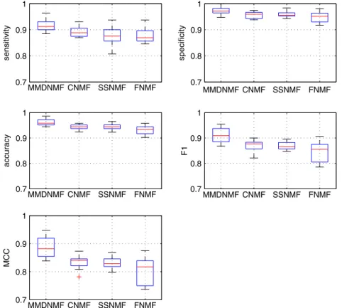
Fig. 1. Experimental results on the bacterial type IVB secreted effector protein data set.
FNMF and SSNMF algorithms, we selected the optimal parameter values from a candidate parameter value pool containing values 3
,
5,
10,
20,
50 and 100. Given a training set containing nine folds, we applied the algorithms with different parameter values from the pool on eight folds, and tested it on the remaining one fold. The procedure was repeated nine times using nine different folds as test fold, and the average accuracies were calculated. The pa-rameter value which obtained the highest average accuracy was chosen. Please note that the chosen value of the same parameter may vary for different training sets. For example, for the FNMF al-gorithm, the basis vector numbers chosen by the ten training set are 5,
10,
20,
100,
10,
50,
5,
10,
20 and 10 respectively. The box-plots of various metrics of ten-fold cross validation are given inFig. 1. We can draw the following conclusions from this figure: 1. It could be easily seen that the proposed MMDNMF outperforms
other NMF methods on various metrics, not only being mea-sured by the median value, but also by the first and third quar-tiles. For example, with regard to the F1 score, only the median value of the F1 scores of MMDNMF is higher than 0.9, while those of all other methods are lower than 0.9. This is a strong ev-idence that applying max–min distance regularization to NMF can explore the class label information more effectively than other methods for the classification purpose.
2. It is also clear that the sensitivity of all methods is lower than their specificity, as shown in the first two subfigures ofFig. 1. It means that it is easier to classify a non-effector protein cor-rectly than to classify an effector protein corcor-rectly. A possible reason is that there are much more non-effector proteins in the data set than the effector proteins.
3. Although there are some differences among CNMF, SSNMF and FNMF, the differences are not significant. A possible reason for this phenomenon is that all the three methods explore the dis-criminative information in a similar way, which weights the class labels of samples equally. For example, FNMF weights the between-class pairs and within-class pairs equally, CNMF forces
the coefficient vectors of samples of the same class to be the same, while SSNMF weights the class label prediction errors of labeled samples equally. FNMF is slightly inferior to CNMF and SSNMF. It is based on the Fisher criterion, which also uses between-class and within-class distances metrics. However, unlike our MMDNMF which forces the minimum between-class distance to be maximized, and also forces the maximum within-class distance to be minimized, FNMF cannot guarantee that the coefficient vectors of samples can be discriminative enough. It indicates that the minimum between-class distance and the maximum within-class distance play critical roles in the repre-sentation problem. This conclusion is consistent to that ofBian and Tao(2011).
To put the obtained results into perspective, in this experiment, we also compared the results of the proposed MMDNMF to two state-of-the-art non-NMF-based classification approaches, nearest neighbor (NN) classifier and support vector machine (SVM). The boxplots of accuracies of ten-fold cross validation of MMDNMF, SVM and NN are given inFig. 2. From this figure, we can see that the proposed MMDNMF obtained the best results, SVM archived com-parable performance, and NN did not obtain good classification re-sults. This means the NMF-based classification methods have good capability for the considered pattern classification problem. A pos-sible reason is that it not only has the capability of representing data, but also has the capability of classifying data. NMF-based clas-sifier can represent the data in a part-based data space effectively and then find a good classification boundary easily.
3.2. Experiment II: hyperspectral image classification
Hyperspectral imaging is a remote sensing technology which allows detailed analysis of the earth surface (Harsanyi & Chang, 1994;Ji et al.,2014;Li, Zhang, Zhang, Huang, & Zhang, 2014; Vill-mann, Merenyi, & Hammer, 2003). Advanced imaging instruments producing high-dimensional images of hundreds of spectral bands
Fig. 2. Comparing the results of MMDNMF to state-of-the-art non-NMF-based classification approaches, SVM and NN, on the bacterial type IVB secreted effector protein data set.
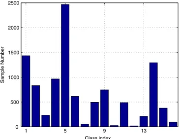
Fig. 3. Number of samples of each class in the Indian Pine data set.
is used by this technology. The classification of each pixel of a hy-perspectral image is of great importance for target detection. In this experiment, the proposed algorithm was evaluated on the problem of hyperspectral image classification.
3.2.1. Data set and protocol
In this experiment, we used a popular hyperspectral image data set—the Indian Pine data set (Chang, Liu, Han, & Chen, 2014;Green et al.,1998;Mukherjee, Bhattacharya, Ghosh, & Arora, 2014). This data set was captured over the Indian test Pines site in Northwest-ern Indiana by the Airborne Visible/Infrared Imaging Spectrometer (AVIRIS) sensor. The image is of spatial dimension of 145
×
145 pix-els, and its spatial resolution is 20 m per pixel. Each pixel is treated as a sample, and it has 220 spectral bands. Moreover, 20 bands con-tained atmospheric noise and water absorption, and were thus re-moved. The remaining 200 bands were used as features for each sample. There were 10366 labeled samples, which were classified into 16 classes. The number of samples of each class varies from 20 to 2468, which is shown inFig. 3.To conduct the experiment, we also performed ten-fold cross validation on the 10366 labeled samples. The experimental results were evaluated by classification accuracy, which is defined as accuracy
=
Number of correctly classified test samplesNumber of test samples
.
(26)3.2.2. Results
The boxplots of the ten-fold cross validation on the Indian Pine data set are shown inFig. 4. From this figure, we can see that the
Fig. 4. Experimental results on the Indian Pine data set.
proposed algorithm, MMDNMF, outperforms the three compared supervised NMF methods again. The median value of the accura-cies of ten-fold cross validation of MMDNMD on this data set is higher than any other compared method. This is a strong evidence of the outperformance of the proposed method over other super-vised NMF methods. The other three compared methods achieve similar performance, but they cannot match the performance of MMDNMF. The reason is as follows: MMDNMF regularizes the fac-torization of data to separate different classes to an extremity. The maximum within-class distance is minimized, and meanwhile the minimum between-class distance is maximized, bringing a large margin between different classes. Compared to MMDNMF, FNMF uses the Fisher rule to separate different classes. It does not push the separation to an extremity as MMDNMF does, thus it is infe-rior to MMDNMF. SSNMF tries to learn the class label directly, and it achieves a similar performance to FNMF. However, this cannot guarantee that the discriminative ability can be explored to an ex-tremity. CNMF also explores the class labels of data samples by forcing the coefficient vectors of the data samples of the same class to a single same one. But it cannot separate the coefficient vectors of different classes effectively. Thus the performance of CNMF is slightly worse than other methods.
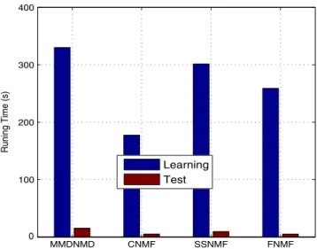
In this experiment, we compared the time costs of different al-gorithms as well. The running time for learning and test proce-dures of the compared algorithms are given inFig. 5. It could be observed that the proposed MMDNMF and SSMNF take more run-ning time than the other algorithms for the learrun-ning procedure, due to their extra load to learn the maximum within-class distance and the minimum between-class distance in the coefficient vector space. Moreover, the test procedure also takes a little more time than other algorithms, because it compares the test sample to all the classes for the classification purpose.
3.3. Experiment III: face classification 3.3.1. Data set and protocol
To show the generated features of the proposed algorithm visually, we also add a standard image classification data set, Yale face database (Georghiades), to the experiment. This data set contains images of 15 people, with 11 grayscale face images for each of them. Thus there are 165 face images in this data set. For each person, the face images are of different facial expression or configuration: center-light, w/glasses, happy, left-light, w/no glasses, normal, right-light, sad, sleepy, surprised, and wink.
3.3.2. Results
To perform the proposed MMDNMF algorithm, each image was resized to 32
×
32 pixels and then reshaped to a 1024 dimensional feature vector. We set the number of basis vectors to the number of people, which is 11. By applying the proposed algorithm toFig. 5. Running time of learning and test procedures of compared algorithms on the Indian Pine data set.
this database using ten-fold cross validation, we obtained a basis matrix and a coefficient matrix to represent the face images in the data set. We reshaped the basis vectors in the basis matrix to the size of 32
×
32 to show the generated features, which are given inFig. 6(a). To obtain the presented results, 100 iterations wereneeded by the proposed MMDNMF algorithm. From this figure, we can see that the learned basis images also have the patterns of face, and are very representative and discriminative for the classification of people in the data set. This indicates that using the criteria of maximizing the minimum between-class distance and minimizing the maximum within-class distance in the coefficient vector space can improve the discriminative ability of the learned representations, as is shown inFig. 6(b).
Since the proposed MMFNMF is an iteration algorithm, the number of iterations has to be chosen such that the algorithm is converged. We also investigated the effect of the number of iterations. The curves of cost functions and accuracies against the number of iterations are shown inFig. 7. From this figure, we can see that when the iteration number is increased from 20 to 500, the cost function is reduced significantly and the classification is also improved significantly. When the iteration number is larger than 1000, both the cost function and the accuracy seem to be stable. This indicates that the algorithm may converge at an iteration number of 500–1000.
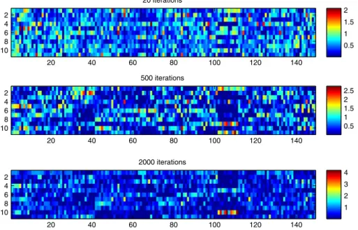
We are also interested in knowing if more iterations make the solution sparse. The learned coefficient matrices with iteration numbers of 20, 500, and 2000 are shown inFig. 8. From this figure, we can see that if the number of iterations is chosen to be small, e.g. 20, a dense coefficient matrix will emerge as shown in the first line ofFig. 8, whereas a large number of iterations will result in a sparse coefficient matrix, as shown in the last line ofFig. 8.
(a) Basis face images learned.
(b) Coefficient matrix.
Fig. 6. Generated features by MMDNMF on the face image data set.
(a) Curve of cost function. (b) Curve of accuracy.
Fig. 8. Coefficient matrices learned by MMDNMF with different number of iterations on the Yale face image data set. 4. Conclusion
In this paper, we investigated how to use the class labels of the data samples to improve the discriminative ability of their NMF representations. To explore the class label information of the data samples, we consider the within-class sample pairs with the same class labels and the between-class sample pairs with differ-ent class labels. Appardiffer-ently, in the NMF represdiffer-entation space, we need to minimize the distances between the within-class pairs, and also maximize the distances between the between-class pairs. In-spired by the max–min distance analysis (Bian & Tao, 2011), we also consider the extreme situation: we pick up the maximum within-class distance and then try to minimize it, so that all the within-class distances are also minimized, and we pick up the minimum between-class distance and then maximize it, so that all the between-class distances are maximized. In contrast to the max–min distance analysis, which only picks up the maximum between-class distance and minimize it, we consider both the between-class and within-class distances simultaneously. Exper-iments on three real world pattern classification problems showed its outperformance over the state-of-the-art supervised and semi-supervised NMF methods.
Acknowledgment
This study was supported by King Abdullah University of Sci-ence and Technology (KAUST), Saudi Arabia.
References
Agarwal, S., Awan, A., & Roth, D.(2004). Learning to detect objects in images via a sparse, part-based representation.IEEE Transactions on Pattern Analysis and Machine Intelligence,26(11), 1475–1490.
Altman, D., & Bland, J.(1994). Diagnostic tests 1: Sensitivity and specificity.British Medical Journal,308(6943), 1552.
Bach, F. R., Lanckriet, G. R., & Jordan, M. I.(2004). Multiple kernel learning, conic duality, and the smo algorithm. InProceedings of the twenty-first international conference on machine learning(p. 6). ACM.
Bhasin, M., & Raghava, G.(2004). ESLpred: SVM-based method for subcellular localization of eukaryotic proteins using dipeptide composition and PSI-BLAST. Nucleic Acids Research,32(2), W414–W419.
Bian, W., & Tao, D.(2011). Max–min distance analysis by using sequential sdp relaxation for dimension reduction.IEEE Transactions on Pattern Analysis and Machine Intelligence,33(5), 1037–1050.
Burman, P. (1989). A comparative study of ordinary cross-validation, v-fold cross-validation and the repeated learning-testing methods.Biometrika,76(3), 503–514.
Cai, D., He, X., Han, J., & Huang, T. S.(2011). Graph regularized nonnegative matrix factorization for data representation.IEEE Transactions on Pattern Analysis and Machine Intelligence,33(8), 1548–1560.
Chang, Y.-L., Liu, J.-N., Han, C.-C., & Chen, Y.-N. (2014). Hyperspectral image classification using nearest feature line embedding approach.IEEE Transactions on Geoscience and Remote Sensing,52(1), 278–287.
Chen, C., Chen, L., Zou, X., & Cai, P.(2009). Prediction of protein secondary structure content by using the concept of Chou’s pseudo amino acid composition and support vector machine.Protein and Peptide Letters,16(1), 27–31.
Chothe, S., & Saxena, H.(2014). Innovative modifications to rose bengal plate test enhance its specificity, sensitivity and predictive value in the diagnosis of brucellosis.Journal of Microbiological Methods,97(1), 25–28.
Congalton, R.(1991). A review of assessing the accuracy of classifications of remotely sensed data.Remote Sensing of Environment,37(1), 35–46. Dang, C., & Xu, L.(2001). A globally convergent Lagrange and barrier function
iterative algorithm for the traveling salesman problem.Neural Networks,14(2), 217–230.
Dentcheva, D., & Ruszczyski, A.(2004). Optimality and duality theory for stochastic optimization problems with nonlinear dominance constraints.Mathematical Programming,99(2), 329–350.
Diewert, W. E. (1974). Applications of duality theory. Stanford Institute for Mathematical Studies in the Social Sciences.
Eches, O., & Guillaume, M. (2014). A bilinear–bilinear nonnegative matrix factorization method for hyperspectral unmixing.IEEE Geoscience and Remote Sensing Letters,11(4), 778–782.
Gao, Y., & Church, G.(2005). Improving molecular cancer class discovery through sparse non-negative matrix factorization.Bioinformatics,21(21), 3970–3975. Gaujoux, R., & Seoighe, C.(2012). Semi-supervised nonnegative matrix factorization
for gene expression deconvolution: A case study. Infection, Genetics and Evolution,12(5), 913–921.
Georghiades, A.Yale face database. Center for computational Vision and Control at Yale University,http://vision.ucsd.edu/content/yale-face-database.
Green, R., Eastwood, M., Sarture, C., Chrien, T., Aronsson, M., Chippendale, B., et al.(1998). Imaging spectroscopy and the airborne visible/infrared imaging spectrometer (aviris).Remote Sensing of Environment,65(3), 227–248. Guillamet, D., Vitri, J., & Schiele, B.(2003). Introducing a weighted non-negative
matrix factorization for image classification.Pattern Recognition Letters,24(14), 2447–2454.
Harsanyi, J. C., & Chang, C.-I. (1994). Hyperspectral image classification and dimensionality reduction: an orthogonal subspace projection approach.IEEE Transactions on Geoscience and Remote Sensing,32(4), 779–785.
Hoyer, P. O.(2004). Non-negative matrix factorization with sparseness constraints. The Journal of Machine Learning Research,5, 1457–1469.
Huang, H., Wang, J., & Abudureyimu, H. (2012). Maximum f1-score discriminative training for automatic mispronunciation detection in computer-assisted language learning, Vol. 1 (pp. 814–817).
Hwang, M., & Kang, H.(2013). A vehicle recognition using part-based representa-tions. InLecture notes in electrical engineering, LNEE:vol. 235(pp. 309–316). Ji, R., Gao, Y., Hong, R., Liu, Q., Tao, D., & Li, X.(2014). Spectral-spatial constraint
hyperspectral image classification.IEEE Transactions on Geoscience and Remote Sensing,52(3), 1811–1824.
Kitamura, D., Saruwatari, H., Iwao, Y., Shikano, K., Kondo, K., & Takahashi, Y. (2013). Superresolution-based stereo signal separation via supervised nonnegative matrix factorization.
Lee, D. D., & Seung, H. S.(1999). Learning the parts of objects by non-negative matrix factorization.Nature,401(6755), 788–791.
Lee, H., Yoo, J., & Choi, S.(2010). Semi-supervised nonnegative matrix factorization. IEEE Signal Processing Letters,17(1), 4–7.
Lemme, A., Reinhart, R. F., & Steil, J. J.(2012). Online learning and generalization of parts-based image representations by non-negative sparse autoencoders. Neural Networks,33, 194–203.
Li, S. Z., Hou, X. W., Zhang, H. J., & Cheng, Q. S.(2001). Learning spatially localized, parts-based representation. InProceedings of the 2001 IEEE computer society conference on computer vision and pattern recognition, 2001, Vol. 1, CVPR 2001. (pp. 1–207). IEEE.
Li, J., Zhang, H., Zhang, L., Huang, X., & Zhang, L.(2014). Joint collaborative representation with multitask learning for hyperspectral image classification. IEEE Transactions on Geoscience and Remote Sensing,52(9), 5923–5936. Lifshitz, Z., Burstein, D., Peeri, M., Zusman, T., Schwartz, K., Shuman, H. A., et al.
(2013). Computational modeling and experimental validation of the legionella and coxiella virulence-related type-ivb secretion signal.Proceedings of the National Academy of Sciences,110(8), E707–E715.
Lin, C.-J.(2007). Projected gradient methods for nonnegative matrix factorization. Neural Computation,19(10), 2756–2779.
Liu, H., Fan, N., & Pardalos, P.(2012). Generalized lagrange function and generalized weak saddle points for a class of multiobjective fractional optimal control problems.Journal of Optimization Theory and Applications,154(2), 370–381. Liu, T., Geng, X., Zheng, X., Li, R., & Wang, J.(2012). Accurate prediction of protein
structural class using auto covariance transformation of PSI-BLAST profiles. Amino Acids,42(6), 2243–2249.
Liu, H., Wu, Z., Li, X., Cai, D., & Huang, T. S.(2012). Constrained nonnegative matrix factorization for image representation.IEEE Transactions on Pattern Analysis and Machine Intelligence,34(7), 1299–1311.
Liu, W., Zheng, N., & You, Q.(2006). Nonnegative matrix factorization and its applications in pattern recognition.Chinese Science Bulletin,51(1), 7–18. Lootsma, F.(1994). Alternative optimization strategies for large-scale
production-allocation problems.European Journal of Operational Research,75(1), 13–40. Malley, C., Braban, C., & Heal, M.(2014). The application of hierarchical cluster
analysis and non-negative matrix factorization to European atmospheric monitoring site classification.Atmospheric Research,138, 30–40.
Mohammadiha, N., Smaragdis, P., & Leijon, A.(2013). Supervised and unsupervised speech enhancement using nonnegative matrix factorization.IEEE Transactions on Audio, Speech and Language Processing,21(10), 2140–2151.
Monga, V., & Mihak, M.(2007). Robust and secure image hashing via non-negative matrix factorizations.IEEE Transactions on Information Forensics and Security, 2(3), 376–390.
Mukherjee, K., Bhattacharya, A., Ghosh, J., & Arora, M. (2014). Comparative performance of fractal based and conventional methods for dimensionality reduction of hyperspectral data.Optics and Lasers in Engineering,55, 267–274. Ou, Y.-Y., Chen, S.-A., & Gromiha, M. M.(2010). Classification of transporters using
efficient radial basis function networks with position-specific scoring matrices and biochemical properties.Proteins-Structure Function and Bioinformatics, 78(7), 1789–1797.
Pascual-Montano, A. (2008). Non-negative matrix factorization in bioinformatics: Towards understanding biological processes (pp. 1332–1335).
Prendiville, R., Pierce, K., & Buckley, F.(2010). A comparison between holstein-friesian and jersey dairy cows and their f1 cross with regard to milk yield, somatic cell score, mastitis, and milking characteristics under grazing conditions.Journal of Dairy Science,93(6), 2741–2750.
Rojatkar, D., Chinchkhede, K., & Sarate, G. (2013). Handwritten devna-gari consonants recognition using mlpnn with five fold cross validation (pp. 1222–1226).
Sandler, R., & Lindenbaum, M.(2011). Nonnegative matrix factorization with earth mover’s distance metric for image analysis.IEEE Transactions on Pattern Analysis and Machine Intelligence,33(8), 1590–1602.
Schneider, M., Bairoch, A., Wu, C. H., & Apweiler, R.(2005). Plant protein annotation in the uniprot knowledgebase.Plant Physiology,138(1), 59–66.
Seung, D., & Lee, L.(2001). Algorithms for non-negative matrix factorization. Advances in Neural Information Processing Systems,13, 556–562.
Shashua, A., & Hazan, T.(2005). Non-negative tensor factorization with applications to statistics and computer vision. InProceedings of the 22nd international conference on machine learning(pp. 792–799). ACM.
Stump, D., Pumplin, J., Brock, R., Casey, D., Huston, J., Kalk, J., Lai, H., & Tung, W. (2001). Uncertainties of predictions from parton distribution functions. i. The lagrange multiplier method.Physical Review D,65(1), 014013.
Tian, L.-P., Liu, L., & Wu, F.-X. (2013). Matrix decomposition methods in bioinformatics.Current Bioinformatics,8(2), 259–266.
Tsarev, D., Petrovskiy, M., & Mashechkin, I. (2011). Using NMF-based text summarization to improve supervised and unsupervised classification. In
Proceedings of the 2011 11th international conference on hybrid intelligent systems, HIS 2011(pp. 185–189).
Van Hamme, H.(2012). An on-line NMF model for temporal pattern learning: Theory with application to automatic speech recognition. InLecture notes in computer science, LNCS:vol. 7191(pp. 306–313). Including subseries Lecture notes in artificial intelligence and lecture notes in bioinformatics.
Vidar, E. A., & Alvindia, S. K. (2013). SVD based graph regularized matrix factorization. InIntelligent data engineering and automated learning—IDEAL 2013 (pp. 234–241). Springer.
Villmann, T., Merenyi, E., & Hammer, B.(2003). Neural maps in remote sensing image analysis.Neural Networks,16(3–4), 389–403.
Wang, J.-Y., Almasri, I., & Gao, X.(2012). Adaptive graph regularized nonnegative matrix factorization via feature selection. In2012 21st international conference on pattern recognition (ICPR)(pp. 963–966). IEEE.
Wang, J. J.-Y., Bensmail, H., & Gao, X.(2013). Multiple graph regularized nonnegative matrix factorization.Pattern Recognition,46(10), 2840–2847.
Wang, J. J.-Y., & Gao, X. (2014). Beyond cross-domain learning: Multiple-domain nonnegative matrix factorization.Engineering Applications of Artificial Intelligence,28, 181–189.
Wang, Y., & Jia, Y.(2004). Fisher non-negative matrix factorization for learning local features. InProc. Asian conf. on comp. vision. Citeseer.
Wang, J., & Qiao, J.(2014). Parameter selection of svr based on improvedk-fold cross validation.Applied Mechanics and Materials,462–463, 182–186.
Wang, J. J.-Y., Wang, X., & Gao, X.(2013). Non-negative matrix factorization by maximizing correntropy for cancer clustering.BMC Bioinformatics,14(1), 107. Wu, H.(2010). Duality theory for optimization problems with interval-valued
objective functions.Journal of Optimization Theory and Applications,144(3), 615–628.
Xu, H., Hui, S., & Grannis, S.(2014). Optimal two-phase sampling design for comparing accuracies of two binary classification rules.Statistics in Medicine, 33(3), 500–513.
Zhang, Z.-W., Xia, K.-W., Yang, F., & Yang, R.-X.(2007). Supervised non-negative matrix factorization algorithm for face recognition.Guangdianzi Jiguang/Journal of Optoelectronics Laser,18(5), 377–389.
Zhao, X., Li, X., Wu, Z., Fu, Y., & Liu, Y.(2013). Multiple subcategories parts-based representation for one sample face identification.IEEE Transactions on Information Forensics and Security,8(10), 1654–1664.
Zheng, C.-H., Zhang, L., Ng, V. T.-Y., Shiu, C. K., & Huang, D.-S.(2011). Molecular pattern discovery based on penalized matrix decomposition. IEEE/ACM Transactions on Computer Biology Bioinformatics,8(6), 1592–1603.
Zhou, Z.-H., & Schwenker, F. (2013). Lecture notes in computer science: Vol. 8183. Partially supervised learning—2nd IAPR international workshop, PSL 2013, revised selected papers(pp. 3–5). Including subseries lecture notes in artificial intelligence and lecture notes in bioinformatics, LNAI.
Zhu, Y.-L. (2008). Sub-pattern non-negative matrix factorization based on random subspace for face recognition. InProceedings of the 2007 international conference on wavelet analysis and pattern recognition, ICWAPR’07, Vol. 3 (pp. 1356–1360). Zou, L., Nan, C., & Hu, F.(2013). Accurate prediction of bacterial type iv secreted effectors using amino acid composition and pssm profiles. Bioinformatics, 29(24), 3135–3142.
Zou, L., Nan, C., & Hu, F.(2013). Accurate prediction of bacterial type iv secreted effectors using amino acid composition and pssm profiles. Bioinformatics, btt554.