Long-Term Sales Forecasting Using Lee-Carter And Holt-Winters Methods

Long-Term Sales Forecasting Using

Lee-Carter And Holt-Winters Methods

Wassana Suwanvijit, Thaksin University, Thailand Thomas Lumley, University of Washington, USA

Chamnein Choonpradub, Prince of Songkla University (Pattani), Thailand Nittaya McNeil, Prince of Songkla University (Pattani), Thailand

ABSTRACT

This study developed a statistical model for long-term forecasting sparkling beverage sales in the 14 provinces of Southern Thailand. Data comprised the series of monthly sales from January 2000 to December 2004 obtained from the company. We applied a classical Lee-Carter mortality forecasting approach as well as exponential smoothing Holt-Winters with additive seasonality method to log-transformed monthly sales containing season of month and branch location as factors. The model produced excellent estimates in sales predicting for up to 24 future months of 20 branches compared with actual data in each branch during the years 2005-2006. The model also gave more accurate results than using separate forecasting method whereas it was parsimonious in the number of parameters used.

Keywords: Long-term; Sales forecasting; Lee-Carter approach; Holt-Winter method; Sparkling beverage

INTRODUCTION Research aim

he research aims to investigate suitable statistical methods for long-term forecasting of sparkling beverage sales revenue data collected routinely in 14 provinces of Southern Thailand during years 2000-2004, including to demonstrate how each method can be implemented using free available software.

Initial assumption of the paper

Forecasting is about predicting the future as accurately as possible. Sales forecast is the amount of a product that the company actually expects to sell during a specific period. A simplistic but useful approach is to begin with a sales forecast where an initial assumption is made that the future sales trend will follow to historical sales or have a similar pattern. Based on our initial assumption, we can identify the general level of sales. We can also determine whether there is a pattern or trend, such as an increase or decrease in sales revenue

over time.

Reasoning for the focus of the paper

Long-term sales forecasting is a difficult area of management. However, it is a subject of great interest as a result of the persistent tendency of company performance and it is indispensable for business planning and strategy. Forecasts help managers by reducing some of the uncertainty, thereby enabling them to develop more useful plans. It also provides useful information for intelligent business decisions making. Modern organizations require sales forecasts and long-term sales forecasts are used in strategic planning. For these reasons, the long-term sales forecast is the main focus of this paper.

Previous researches

Several statistical models have been used for business data forecasting in the previous researches. Software World (2009) developed computer model for forecasting beer consumption in UK by applying Mathematics techniques of correlation analysis, regression analysis. The model would have been accurate within 10% on 90% of occasions for forecasting monthly consumption. RNCOS (2008) forecast Philippines, beverages and tobacco market till 2011 using ratio analysis, historical trend analysis and linear regression analysis. Information has been sourced from books, newspapers, trade journals, and white papers, industry portals, government agencies, trade associations, monitoring industry news and developments, and through access to more than 3000 paid databases. The report provides detailed overview of the consumption patterns of the Philippines in various food segments. The beverage segment talks about the type of beverages, their sales and consumption patterns among Philippines while the tobacco segment provides a brief description of the tobacco industry in the country. Boonruangthaworn (2007) studied about forecasting techniques for soft drink industry in order to predict the demand of a new product so that the production planning and inventory control are more efficient. They collect the historical demand data from 2004 to 2006. Then, implement both qualitative and quantitative forecasting models and compare their forecasting error such as MSE, MAD and MAPE. Then, the best model is selected as an input of the production planning. Finally, they compare total cost by using the result from both techniques. The results show that Least Square is the best forecasting method with the lowest forecasting error. In addition, by using this technique, the related cost can be reduced by 90% compared to that of the current technique. The result show that this quantitative forecasting technique is more appropriate than the current qualitative forecasting technique by considering cost and service level criteria. Higgins et al. (2005) analysis the residual demand to test whether carbonated soft drinks is a relevant product market using weekly A.C. Nielsen Scanner price and quantity data for carbonated soft drink products purchased in supermarkets in the United States. The results suggest that a market for carbonated soft drinks is too narrow for purposes of merger analysis according to the Merger Guidelines established by the United States Department of Justice and the Federal Trade Commission. In the case study of carbonated soft drink consumption and bone mineral density in adolescence by McGartland et al (2003), adjusted regression modeling was used to investigate the influence of carbonated soft drinks on bone mineral density. Lin et al (2002) forecasted non-alcoholic beverage sales in Taiwan. The study applied the Grey dynamic model to forecast sales of eight sub-category non-alcoholic beverages in Taiwan between 2001 and 2003. The accuracy of the new forecasting model exceeds 95 percent. The model estimates that the total beverages market will grow, but growth rates will vary for individual sub-categories. In relation to current growth, from 2001 to 2003, tea drinks, carbonated drinks, functional drinks and sports drinks will experience decreased market growth, while bottled water and fruit and vegetable juices will be a high growth market and coffee drinks and other drinks will enjoy improved sales. These results provide a valuable reference for the Taiwanese beverage industry developing marketing plans.

Research and epistemological approaches

The research and epistemological approaches that have been adopted to conduct this research are Lee-Carter model and Holt-Winters exponential smoothing method. These are different methods compared with the methods used for sales forecasting in the previous researches. However, these approaches basically involve the theoretical framework that has to be adopted in this study.

Originality of the paper and contribution to knowledge

This study attempts to extend the knowledge about long-term forecasting to produce useful finding for both company and further researches. The originality of the paper lies in the methodologies we apply for long-term forecasting of sparkling beverage sales revenue and the accurate of the sales forecast compared with actual value and the results from using the separate forecast method. A new forecasting model is presented and the model can be extended into other specific business data analysis and forecasting using the same methods.

Area of study

Thailand is divided into four geographical regions. The southern region occupies about 14% of the total land area. There are 14 provinces in southern Thailand with a total area 71,798 square kilometers. Sparkling

beverages are traditionally popular products in the south, although some consumers prefer more healthy beverages. Sparkling beverages are also primarily used as mixers for consumption with alcoholic drinks. There are 20 branches in Southern Thailand. The branch locations are shown in Figure 1.

Figure 1. Branch Locations in Southern Thailand

Preliminary analysis and results

The monthly sales revenue was plotted to assess trend and branch effects before choosing the best model for forecasting. Let





x x

x



b







log

Figure 2 shows the result from the linear regression fitted given by (1) in the left panel and the time series plot of some branches in the right panel. The preliminary analysis using historical data indicates that the monthly sales in each branch location have increased substantially. However, each branch has different patterns in the growth rate compared with the others. The branch location is a factor of interest in the models since it affects the sales trend. The time series plot also shows seasonal effect on the sales in each branch.

Figure 2: Monthly sales by branch (left panel) and time series plot by branch (right panel)

THEORETICAL FRAMEWORK

In this study, the statistical method for long-term sales forecasting was selected based on empirically tested theories (Baker 1999). Figure 3 shows theoretical basis of the study. The theoretical perspective in this study is based on statistical forecasts using extrapolation models and quantitative forecasting method. Quantitative forecasting methods are used when historical data on variables of interest are available. These methods are based on an analysis of historical data concerning the time series of the specific variable of interest and possibly other related time series. It is preferable to use this method rather than judgmental extrapolations because extrapolation methods become more useful and less expensive as one can work directly with time-series data on sales. Extrapolation methods use only historical data on the series of interest and quantitative extrapolation methods make no use of managements’ knowledge of the series. The theory assumes that the causal forces that have affected a historical series will continue over the forecast horizon. Extrapolation of sales can be used to predict for the situation that is of interest that often adequate for the decisions that need to be made.

Statistical

Univariate

Figure 3: Theoretical basis of study

RESEARCH MODEL

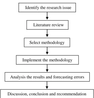
Steps to forecast are: 1) decide what to forecast, 2) evaluate & analyze appropriate data, 3) select & test the forecasting model, and 4) generate the forecast and monitor forecast accuracy over time. Figure 4 shows the research model of this study. We indentify what to forecast and research aims in the first step. Then, the in depth

Knowledge Source

Extrapolation Models

literature review and literature review are explored. Next, we select the right sales forecast methodology based on empirically tested theories. After that, we implement the forecasting methodology including to evaluate and analyze the forecasting results and the errors in order to find the suitable model. Finally, we do the discussion, summary and recommendation for further studies.

Figure 4: Research model of study

LITERATURE REVIEWS

From the theoretical framework as shown in Figure 3, the theoretical perspective in this study is based on statistical forecasts using extrapolation models and quantitative forecasting method. The non-linear Lee-Carter approach was designed for long-term forecasting based on a lengthy time series of historic data. The most popular and cost effective of extrapolation models and quantitative forecasting method are based on exponential smoothing, which implements the useful principle that the more recent data are weighted more heavily. The Holt-Winters exponential weight method is also popular for long-term forecasting of business data. Therefore, a classical Lee-Carter mortality forecasting approach and exponential smoothing Holt-Winters method were applied for long-term sales forecast in this study.

The non-linear Lee-Carter approach (Lee and Carter 1992), is widely used in both the academic literature and practical applications and it has become the “leading statistical model of mortality forecasting in the demographic literature” (Deaton and Paxson 2004). The method was designed for long-term forecasting based on a lengthy time series of historic data. In the typical application, this model is fitted to past data to obtain parameter estimates, then it produces an excellent fit to mortality trends by linearized trends and thereby adds confidence to extrapolations. Since the Lee-Carter model is computationally simple to apply and it has given successful results, it was popular used for long-term forecasts of age specific mortality rates from various countries and time periods, such as USA (Lee and Carter 1992), Canada (Lee and Nault 1993), Chile (Lee and Rofman 1994), Japan (Wilmoth 1996), the seven most economically developed nations (G7) (Tuljapurkar et al 2000), Belgium (Brouhns et al 2002) and Sweden (Wang 2007). The model can also be applied for seasonality and non-linearity data such as using to price a risky coupon survivor bond (Denuit et al 2007) including to describe seasonal variation and non-linear for quarterly industrial production (Franses et al 2005). The original principal component of the Lee -Carter model is

x x _{t xt} (2)

t

x a bk

m_,) _,

log(   



Identify the research issue

Literature review

Select methodology

Implement the methodology

Discussion, conclusion and recommendation Analysis the results and forecasting errors

with mortality mx,t at age x and time t, fixed age effect ax equal to the average observed log death rate and an

age-specific impact bx of a time-specific general mortality index kt , where is a set of random disturbances. This

single parameter kt maps as the average age pattern of mortality deviation from ax to the actual pattern. bx is the first

principle component which is estimated by singular value decomposition method. Constraints imposed to obtain a unique solution are the bx sum to unity and the kt sum to zero. The subsequent estimation of the mortality index kt as

a time series linear forecasting model: ARIMA (autoregressive integrated moving average) process results in a simple random walk with drift. The method adjusts kt by refitting to total observed deaths.

The underlying principle of the Lee-Carter method is the extrapolation of past trends and makes no effort to incorporate knowledge about medical, behavioral, or social influences on mortality change. This method allows age-specific death rates to decline exponentially without limit and assumes that the model errors have the same variance over all ages. Several advantages of the model are claimed such as a parsimonious demographic model is combined with statistical time-series methods, the method involves no subjective judgments, forecasting is based on persistent long-term trends and probabilistic confidence intervals are provided for the forecasts (Lee and Carter 1992). The model is also computationally simple to apply with robustness in the context of linear trends in age-specific death rates. Differ criteria have been proposed for the Lee-Carter method. Wilmoth (1993) developed two alternative one-stage estimation strategies which are a weighted least square (WLS) and a maximum likelihood (MLE) technique. Bell (1997) suggested using a multivariate time series model for all coefficients and do not exploit the orthogonality of the coefficient series. There have been several extensions of the Lee-Carter method such as non-parametric smoothing, Kalman filtering, and multiple principle components.

Exponential smoothing is a procedure for continually revising a forecast in the light of more recent experiences. Exponential smoothing assigns exponentially decreasing weights as the observation get older. In other words, recent observations are given relatively more weights in forecasting than the older observations (Kalekar 2004). Exponential smoothing methods are among the most widely used forecasting techniques in industry and business, in particular the well-known Holt-Winters methods (Holt 1957 and Winters 1960) that allow us to deal with univariate time series with contain both trend and seasonally factors. Their popularity is due to their simple model formulation and good forecasting results (Gardner 1985). Holt-Winters is popular for mass produced forecasts, for example in production planning, because of its simplicity (ONS 2008). Kotsialos et al (2005) used of a damped-trend Holt-Winters method and feedforward multilayer neural networks to forecast sales data from two German companies up to 52 periods ahead. Bermudez et al (2005) applied additive Holt-Winters forecasting procedure to the series of monthly total UK air passengers from the year 1949 to 2005. Newberne (2007) demonstrated the use of the Holt-Winters model on common healthcare data series.

METHODOLOGIES Research method

This quantitative research focused on the classical Lee-Carter model and the well-known Holt-Winters with additive seasonality method to log-transformed monthly sales containing season of month and branch location as factors. We fitted the models to the data. Then, the models of sales revenue, which contains trend and seasonal effects were applied to estimate in sales predicting for up to 24 future months of 20 branchesin Southern Thailand. All graphical and statistical analyses were performed using R (R development core team 2008).

Procedure and data collection

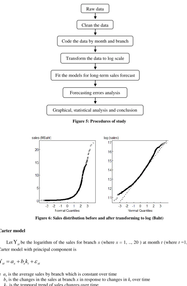
Figure 5 show procedures in this study. Monthly data was available in computer files with records for sales revenue separated by branch location. After correcting or imputing data entry errors, records from years 2000 to 2004 were stored in a MySQL database. MySQL and Excel programs were used to create sales revenue in Baht by month and branch location. Sales revenues generally have skewed distributions, so it is essential to transform them by taking logarithms. Log-transformations can also ensure that statistical assumptions of symmetry and variance homogeneity of errors are satisfied. Figure 6 shows the overall distribution before and after transforming the data by taking logarithms of the sales. It shows that the distribution is more symmetric after transforming the data.

t x,

Figure 5:Procedures of study

Figure 6: Sales distribution before and after transforming to log (Baht)

Lee-Carter model

Let



xt t x x xt



a



b

k







log

where ax is the average sales by branch which is constant over time

bx is the changes in the sales at branch x in response to changes in kt over time kt is the temporal trend of sales changes over time

εxt is a vector of error terms

Raw data

Clean the data

Code the data by month and branch

Transform the data to log scale

Fit the models for long-term sales forecast

Forecasting errors analysis

with the constraints: (4)

Lee-Carter model with 2 components extension can be written as

xt t x t x x xt



a



b

k



b

k







log

Lee-Carter model with 3 components extension can be written as

xt t x t x t x x xt



a



b

k



b

k



b

k







log

We estimated the average sales (ax) by

(7)

For the least squares estimation, the Singular Value Decomposition (given by the R function “svd”) was applied to the average sales over time t for each branch x.

(8)

where D is a diagonal matrix containing singular values and both U and V are orthogonal matrices. The parameters bx1, bx2, bx3 are set equal to the first, second and third column of U respectively, and the kt1, kt2, kt3 values are set equal to the product of the first, second and third column of V and the leading singularvalue d1, d2, d3 respectively along with the normalizations given in (4). In order to make more accurate in the forecasting results, we adjust bx1, bx2, bx3 by comparison with an average of the last 12 months observation data.

In the next step, we fitted the Lee-Carter model given by (3), (5) and (6) by using estimated parameters including to the bx1, bx2, bx3 adjustedfrom the previous step. Then we compared the results from fitting the Lee-Carter model with the 60 months observation data. After that we adjust kt1, kt2, kt3 for the best fit of each model. The estimated parameters for the Lee-Carter model with 1-3 components are shown in Figure 7.

Figure 7: Parameters (ax, bx1, bx2, bx3, kt1, kt2 and kt3) for the Lee-Carter model plots

Holt-Winters method

Since the historical data series are seasonal with linear trend, we forecast kt1, kt2, kt3 adjusted values for up to 24 months ahead as well as their 95% robust prediction intervals by using Holt-Winters exponential smoothing with additive seasonality forecasting method. The Holt-Winters prediction function (for time series with period length p) is

K

ˆ



a



hb



s





,

log





a



UD

V









a

log

where at, bt and st are given by at = α (Kt - st-p) + (1- α) (at-1+ bt-1)

bt = β (at – at-1) + (1- β) bt-1

st = r(Kt - at ) + (1- r) st-p

Once kt1, kt2, kt3 forecast are built, the monthly sales forecast in each branch can be predicted easily by just fitting the Lee-Carter model using kt1, kt2, kt3 forecasted as well as ax given by (7) and the bx1, bx2, bx3 adjusted. So,

let z be the 24 months in the future, the prediction of



z t x z t x z t x z t x x z t x 



a



b

k



b

k



b

k





ˆ

log



As Baker (1992) pointed out that traditional error measures, such as mean square error, do not provide a reliable basis for comparison of methods. The Mean Absolute Percentage Error (MAPE) is more appropriate because it is invariant to scale and is not overly influenced by outliers. For comparisons using a small set of series, it is desirable, also, to control for degree of difficulty in forecasting. For these reasons, as a measure of fitting and forecast accuracy of each model and compared with separate forecasts by branch, we compute the mean absolute error (MAPE) from

(11)

Analyses

In the analysis, we simply take the quantitative measures of the forecasting results. We seek to the suitable statistical model by comparing the forecasting results with the actual value during years 2005-2006 and the results from using separate forecast method, including to measure the forecasting errors of each model.

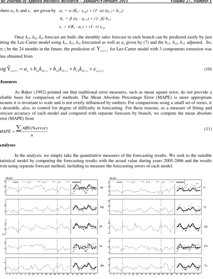
Figure 8: Forecasting results using Lee-Carter models 1-3 components compare with the results from using separate forecast method

n error ABS

RESEARCH RESULTS

In order to find the best model for long-term sales forecasting, we fitted the Lee-Carter 1-3 components compare with separate forecast including to the actual data during years 2005 -2006 (24 months). The forecasting results of some branches can be compared in Figure 8. As can be seen from Figure 8 that the predicted lines of each model is quite closed to the actual values. However, the forecasting results using the Lee-Carter model with 3 components extension can give the best fit than other models and there are some forecasting errors that need to be considered in the next step.

Forecasting errors

As can be seen from Figure 8 that there is a rapid trend in Yala branch during the years 2005-2006 that may caused high forecasting errors. So, we evaluated the forecast accuracy by comparison both the total forecasting error and the errors excluding the Yala (Yl) branch from the formulas given by (11). The forecasting errors are shown in Table 1. The table shows that the mean absolute percent error from using the Lee-Carter model with 3 components extension is less than using the other model or the separate method. The errors from forecasting sales in 19 branches (exclude Yala branch) are less than from forecasting sales in all branch locations.

Table 1: Forecasting errors comparison between each model

Methods Mean absolute percent error (MAPE)

Total Excl. Yala branch

Lee-Carter 1 component 1.52% 1.35%

Lee-Carter 2 components 1.35% 1.20%

Lee-Carter 3 components 1.32% 1.16%

Separate forecast 1.47% 1.39%

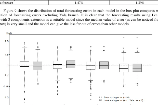
Figure 9 shows the distribution of total forecasting errors in each model in the box plot compares with the distribution of forecasting errors excluding Yala branch. It is clear that the forecasting results using Lee-Carter model with 3 components extension is a suitable model since the median value of error (as can be noticed from line in the box) is very small and the model can give the less far out of errors than other models.

Figure 9:Forecasting errors of each model in total compare with the errors exclude Yala branch

From the forecasting errors analysis as shown in table 1 and Figure 9, we found that the Lee-Carter model with 3 components extension was the best model for long-term forecasting of sparkling beverages sales in Southern Thailand.

Prediction Interval

It is useful to consider the 95% prediction intervals with the point forecast. Figure 10 shows some of the forecasting results with 95% prediction intervals comparison between Lee-Carter model with 3 components extension and separate forecasts. As can be seen from Figure 10 that although there are some of the observed data are outside of the predicted lines but they are well-covered by the prediction intervals. The plot displays that the forecasting results using the Lee-Carter model with 3 components extension are well-covered by the prediction intervals than the separate method.

Figure 10: The forecast results using Lee-Carter 3 components with 95% prediction interval compare with the results from using separate forecast and actual data

Figure 11 shows the scatter plot comparison between actual sales in the forecasting periods (January 2005 to December 2006) and 24 months predicted sales in 20 branches. The plot indicates that the forecasting results are well fit to the actual value and the smoothing line.

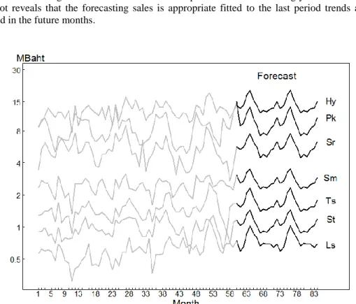
Figure 12 shows time series of the actual sales during years 2000 - 2004 (60 months) and the sales forecast of some branches from fitting Lee-Carter model with 3 components extension during years 2005 – 2006 (24 months ahead). The plot reveals that the forecasting sales is appropriate fitted to the last period trends and can give the reasonable trend in the future months.

Figure 12: Monthly actual sales by branch with 24 future months sales forecasting using the Lee-Carter model with 3 components extension

DISCUSSION

The sales in each branch have increased substantially. This could be due to an expansion in modern trade outlets affecting purchasing behaviours and consumers life style in Southern Thailand. There is a significant sales growth in Yala branch during the forecasting periods due to the market execution and distribution penetration by the company. So, it is a good opportunity for the company to focus and do some more promotions or marketing strategies especially for this area.

The seasonal effects found in our study could be related both to regional climatic changes and to human activities. In the dry season (extending from February to April), hot weather and long holidays lead to greater consumption of sparkling beverages.

Degree of answering the research objectives and the support of the initial assumptions

Forecasting is an active research area for many decades. The accuracy of forecasting hence researchers for improving the effectiveness of forecasting models. In this paper, we applied a Lee-Carter model with 3 components extension and exponential smoothing Holt-Winters with additive seasonality method for sparkling beverages sales data with logarithmic transformation. This is a suitable case-study since the model produced excellent estimates in sales predicting for up to 24 future months of 20 branches compared with actual data in each branch during the years

2005 - 2006. As can be seen from table 1 that the model gave more accurate results than using separate forecasting method. The Lee-Carter model takes advantage of the unique strength of non-linear modeling and it produces an excellent fit and sensible estimates in long-term sales predicting for many branches in the same time. It is also parsimonious in the number of parameters used and its concept is not much complicated for a person with minimal knowledge of statistics. The exponential smoothing Holt-Winters with additive seasonality method allows us to deal with univariate time series with contain both trend and seasonally factors. It contains simple model formulation and can give good forecasting results.

The model can support of the initial assumptions that the future sales trend will follow to historical sales or have a similar pattern. The model can also support our research aims in investigating suitable statistical methods for long-term sales forecasting and implementing the method using free available software (R).

Relating the findings to earlier work

In the previous researches or earlier works, the long-term sales forecasts usually work by using the separate forecasting methods. For example, in this case forecasters need to forecast the sales in each branch location separately or do the 20 times forecasts. This study attempted to extend the knowledge about long-term forecasting through the development of a statistical model. By using such our model, the forecasters can save the forecasting time and cost since it is needs only one time fitting the forecasting model given by (10), to achieve the sales forecast for up to 24 future months of 20 branches.

Theoretical implications

The models can be extended into other specific business data analysis and forecasting using the same methods and theoretical framework.

Practical implications

For practical use, the model is designed to deal with the following two points: accuracy and timing used. As a case study, we applied the model to sparkling beverages sold in Southern Thailand. The model enables us to obtain a practical sales forecast in 20 branches, and furthermore provides valuable information on reprint decision-making. Using such models for forecasting sales revenue can assist company managers in long-run planning more effectively.

Limitations

There is a limitation of the Lee-Carter model that the model is well-fitted in case of the sales trend in each branch has a similar pattern. As can be noticed from the Yala branch case, the forecasting results was not good enough due to there was a rapid sales growth during the predicting periods which was a different trend compared with other branches. Some substantial interactions between the branch-month factor and the other factors existed could not be fitted using the model. In addition, the forecasting results using Holt-Winters method always depend on the last period trend.

Recommendation for further researches

For further studies, sales data in recent year, new packages and new flavours data may be considered in further sales forecast. The models can be easily adapted for per capita consumption forecasting or extended to other business data forecast.

CONCLUSION

In this study, we applied a classical Lee-Carter mortality forecasting approach as well as exponential smoothing Holt-Winters with additive seasonality method to log-transformed monthly sales containing season of month and branch location as factors. By using a basic forecasting process, we found that the Lee-Carter model with

Holt-Winters method can produces an excellent fit and it can give sensible estimates in long-term sales forecasting for 20 branches in the same time. The model also parsimonious in the number of parameters used and its concept is not much complicated for a person with minimal knowledge of statistics. The model also gives more accurate results than using separate forecasting method. The models can be extended into other specific business data analysis and forecasting using the same methods.

ACKNOWLEDGEMENTS

We would like to thank the Office of the Higher Education Commission, Thailand for supporting by grant fund under the program Strategic Scholarships Fellowships Frontier Research Networks (Specific for Southern region) for the Join PhD Program Thai Doctoral degree for this research. We are grateful for Prof. Don McNeil for his helpful advice and suggestions. We also would like to thank Khun Dumrongrugs Apibalsawasdi for his guidance.

AUTHOR INFORMATION

Wassana Suwanvijit: Instructor for the Faculty of Economics and Business Administration, Thaksin University, Songkhla, Thailand and currently a PhD candidate in Research Methodology.

Thomas Lumley, PhD: Professor for the Department of Biostatistics, University of Washington, USA.

Chamnein Choonpradub, PhD: Assistant Professor for the Department of Mathematics and Computer Science, Faculty of Science and Technology, Prince of Songkla University (Pattani campus), Thailand.

Nittaya McNeil, PhD: Instructor for the Department of Mathematics and Computer Science, Faculty of Science and Technology, Prince of Songkla University (Pattani campus), Thailand.

REFERENCES

1. Baker, Michael J. The IEBM Encyclopedia of Marketing, International Thompson Business Press, pp. 278-290, 1999.

2. Bell, W.R. Comparing and assessing time series methods for forecasting age-specific fertility rates, Journal of Official Statistic, Vol. 13, pp. 279-303, 1997.

3. Bermudez, J.D., Segura, J.V. and Vercher, E. Holt-Winters forecasting: an alternative formulation applied to UK air passenger data, Centro de Investigation Operativa(CIO), 2005.

4. Bohr, Neils. and Danish. Introduction to Forecasting, 2007. http://www.answers.com/forecasting?cat=biz-fin [March 12, 2009]

5. Boonruangthaworn, Duangrat. Forecasting Techniques for New Product: Case Study of Soft Drink Industry, 2007. http://aitm.agro.ku.ac.th/students/s01/abstracts/2007_duangrat_en.pdf [January 22, 2008] 6. Booth, H. Demographic Forecasting: 1980 to 2005 in review, International Journal of Forecasting, Vol.

22, pp. 547-581, 2006.

7. Booth, H., Hyndman R.J., Tickle, L. and DeJong, P. Lee-Carter mortality forecasting: a multi-country comparison of variants and extensions, Demographic Research, Vol. 15, pp. 289-310, 2006.

8. Booth, H., Maindonald, J. and Smith, S. Applying Lee-Carter under conditions of variable mortality decline, Population Studies, Vol. 56, pp. 325-336, 2002.

9. Brouhns, N., Denuit, M. and Vermunt, J. A Poisson Log-bilinear Regression Approach to the Construction of Projected Lifetables, Insurance: Mathematics and Economics, Vol. 31, pp. 373-393, 2002.

10. Bureau. Indian Food and Beverages Forecast (2007-2011), June, 2007.

11. Caruana, Albert. Step in forecasting with seasonal regression: A case study from the carbonated soft drink market, Vol. 10, No. 2, pp. 94-102, 2001.

12. Chatfield, C., Koehler, A. B., Ord, J. K. and Snyder, R. D. A new look at models for exponential

smoothing, Journal of the Royal Statistical Society, Series D:The Statistician, Vol. 50, No. 2, pp. 147-159, 2001.

13. Currie, Iain. The Extended Lee-Carter Family, Actuarial Teaching and Research Conference, Queen’s University, 2009.

14. Currie, I.D., Durban, M. and Eilers, P.H.C. Smoothing and forecasting mortality rates. Statistical Modelling, Vol. 4, No. 4, pp. 279-298, 2004.

15. Dekimpe, M. G. and Hanssens, D. M. Time-series models in marketing: Past, present and future. International Journal of Research in Marketing, Vol. 17, pp. 183-193, 2000.

16. Denuit, Michel., Devolder, Pierre. and Goderniaux, Anne-C6cile. Securitization of Longevity Risk: Pricing Survivor with Wang Transform in the Lee-Carter Framework, The Journal of Risk and Insurance, Vol. 74, No. 1, pp. 87-113, 2007.

17. Franses, Philip Hans. and Dijk, Dick Van. The forecasting performance of various models for seasonality and nonlinearity for quarterly industrial production, International Journal of Forecasting, Vol. 21, pp. 87-102, 2005.

18. Gardner, E.S. Jr. Exponential smoothing: the state of the art, Journal of Forecasting, Vol. 4, pp. 1-28, 1985.

19. Gelper, S., Fried, R. and Croux, C. Robust forecasting with exponential and Holt–Winters smoothing, Journal of Forecasting. Vol. 29, No. 3, pp 285-300, 2010.

20. Girosi, Federico. and King, Gary. Understanding the Lee-Carter Mortality Forecasting Method, Working Paper, Harvard University, 2007.

21. Granger, Clive W.J., Jeon, Yongil. Long-term forecasting and evaluation, International Journal of Forecasting, Vol. 23, pp. 539–551, 2007.

22. Girosi, Federico. and King, Gary. Understanding the Lee-Carter Mortality Forecasting Method, Working Paper, Harvard University, 2007.

23. Hanke, John E. and Wichern, Dean W. Business Forecasting, Pearson Education, New Jersy, 2005. 24. Higgins, Richard S., Kaplan, David R. and McDonald, Michel J. Residual Demand Analysis of the

Carbonated Soft Drink Industry, 2005.http://www.springerlink.com/content/h7n6w33821up1w24/ [July 13, 2009]

25. Holt, C.C. Forecasting seasonals and trends by exponentially weighted moving averages, ONR Research Memorandum, Carnigie Institute, Vol. 52, 1957.

26. Hyndman, Rob J. and Ullah Md. Shahid. Robust forecasting of mortality and fertility rates: A functional data approach, Computational Statistics & Data Analysis, Vol. 51, pp. 4942-4956, 2007.

27. Hyndman, Rob J. Business forecasting methods, 2009.

http://www.robjhyndman.com/papers/businessforecasting.pdf [January 22, 2010]

28. Inoue, Atsushi. and Kilian, Lutz. On the selection of forecasting models, Journal of Econometrics, Vol. 130, pp. 273–306, 2006.

29. Jan G. De Gooijer., Rob J. Hyndman. 25 years of time series forecasting, InternationalJournal of Forecasting, Vol. 22, pp. 443-473, 2006.

30. Kalekar, Prajakta S. Time series forecasting using Holt-Winter exponential smoothing, Kanwall Rekhi School of Information Technology, 2004.

31. Koehler, Anne B., Snyder, Ralph D. and Ord, J. Keith. Forecasting models and prediction intervals for the multiplicative Holt-Winters methods. International Journal of Forecasting, Vol. 17, pp. 269-286, 2001. 32. Koissi, M-C., Shapiro, A.F. and Hognas, G., Evaluating and extending the Lee-Carter models for mortality

forecasting: Bootstrap confidence intervals, Insurance Mathematics and Economics, Vol. 38, pp. 1-20, 2006.

33. Kotsialos, Apostlos., Papageorgiou, Markos. and Poulimenos, Antonios. Long-Term Sales Forecasting Using Holt-Winters and Neural Network Methods, Journal of Forecasting, Vol. 24, pp. 353-368, 2005. 34. Lawton, Richard. How should additive Holt-Winters estimates be corrected?, International Journal of

Forecasting, Vol. 14, pp. 393-403, 1998.

35. Lazar, Dorina. On forecasting mortality using Lee-Carter method, Babes Bolyai University, 2004. http://www.stat.ucl.ac.be/Samos2004/proceedings2004/Lazar2.pdf [April 14, 2010].

36. Lee, R.D. and Carter, L. R., Modeling and forecasting U.S. Mortality, Journal of American Statistical Association, Vol. 87, No. 41, pp. 659-671, 1992.

37. Lee, R.D. The Lee-Carter Method for Forecasting Mortality, With Various Extensions and Applications (with discussion), North American Actuarial Journal, Vol. 4, No. 1, pp. 80-93, 2000.

38. Lee, R.D. and Miller, T. Evaluating the performance of the Lee-Carter mortality forecasts, Demography. Vol. 38, pp. 537-549, 2001.

39. Lee, R. D., Nault, F. Modeling and forecasting provincial mortality in Canada, paper presented at the World Congress of the International Union for Scientific Study of Population, Montreal, 1993.

40. Lee, R. D., Rofman, R. Modeling and Projecting Mortality in Chile, Notas Polacion, Vol. 22, No. 59, pp. 183-213, 1994.

41. Lin, Chin-Tsai. and Hsu, Pi-Fang., Forecast of non-alcoholic beverage sales in Taiwan using the Grey theory. Asia Pacific Journal of Marketing and Logistics, Vol.14, No.4, pp.3-12, 2002. 42. McGartland, C., Robson, P.J., Murray, L., Cran, G., Savage, M.J., Watkins, D., Rooney, M., & Roreham,

C. Carbonated Soft Drink Consumption and Bone Mineral Density in Adolescence: The Northern Ireland Young Hearts Project, Journal of bone and mineral research, Vol. 18, pp. 1563-1569, 2003.

43. Newbeme, Joan H. and Captain, USAF. MSC Holt-Winters Forecasting in Healthcare, Mike O' Callaghan Federal Hospital, 2007.

44. ONS. Documentation of UKCeMGA Methods used for National Accounts, 2008. http://www.statistics.gov.uk. [April 14, 2010].

45. Pan, R. Holt–Winters Exponential Smoothing, Wiley Encyclopedia of Operations Research and Management Science, 2010.

46. Racharit, N. and Suraseangsung, S. Forecasting models for Thai Mortality Rates Using the Lee-Carter Method, Journal of Demography, Vol. 22, No. 2, 2006.

47. Renshaw, A.E. and Haberman, S. Lee-Carter mortality forecasting: a parallel generalised linear modeling approach for England and Wales mortality projections, Applied Statistics, Vol. 52, pp. 119-137, 2003. 48. R Development Core Team. R: A Language and Environment for Statistical Computing, R Foundation for

Statistical Computing, Vienna, Austria, 2008.

49. RNCOS. South Korean Food, Beverages and Tobacco Market Forecast till 2011, 2007

50. Software World. Computer model for forecasting beer consumption in U.K. A.P. Publications Ltd. 2009. http://www.thefreelibrary.com [April 14, 2010].

51. Sorin, Sylvain. Exponential weights algolithm in continuous time, Spinger-Virlag, 2007.

52. Steffens, P., Kaya, M. and Albers, S. Long term sales forecasts of innovations - An empirical study of the consumer electronic market, proceedings AGSE Entrepreneurship Research Exchange, 2007.

53. Suwanvijit, W., Choonpradub, C. and McNeil, N. Sales analysis with application to sparkling beverage product sales in Southern Thailand, International Journal of Business and Management, Vol. 4, No. 7, pp. 43-51, 2009.

54. Suwanvijit, W., Choonpradub, C. and McNeil, N. Statistical model for short-term forecasting sparkling beverage sales in Southern Thailand, International Business and Economics Research Journal, Vol. 8, No. 9, pp. 73-81, 2009.

55. Tanaka, K. A sales forecasting model for new-released and nonlinear sales trend products, Expert Systems with Applications, Vol. 37, No. 11, pp. 7387-7393, 2010.

56. Tinney, Mary-Colleen., Retail Sales Analysis: Champagne and Sparkling Wine Sales Rising, Wine Communications Group, 2007.

57. Tuljapurkar, S., Li, N. and Boe, C. A Universal Pattern of Mortality Decline in the G7 Countries, Nature, Vol. 405, pp. 789-792, 2000.

58. Venables, W. N. and Ripley B.D. Modern Applied Statistics withS. Springer, Queensland, 2002. 59. Venables, W. N. and Smith, D.M. An Introduction to R, 2004.

http://cran.r-project.org/doc/manuals/R-intro.pdf [March 30, 2009]

60. Wang, Jenny Zheng. Fitting and Forecasting Mortality for Sweden: Applying the Lee-Carter Model, Mathematical Statistics, Stockholm University, 2007. http://www.math.su.se/matstat [April 4, 2010]. 61. Williams. Developing Sales Forecasts, 2007. http://web.csustan.edu/market/williams/Chapter%2010.htm

[March 14, 2010].

62. Wilmoth, John R. Mortality Projections for Japan: A Comparison of Four Methods, Health and Mortality Among Elderly Populations, Oxford University Press, pp. 266-287, 1996.

63. Wilmoth, J.R. Computational methods for fitting and extrapolating the Lee-Carter model of mortality change. Technical Report. Dept. of Demography, University of California, Berkeley, 1993.

64. Winters, P. R. Forecasting sales by exponentially weighted moving averages, Management Science, Vol. 6, pp. 324–342, 1960.

65. Yelland, P., Kim, S. and Stratulate, R. A Bayesian model for sales forecasting at Sun Microsystems, Interfaces, Vol. 40, No. 2, pp.118-129, 2010.