1
Testing Complex Social Theories with Causal Mediation Analysis and G-Computation – Towards a Better Way to Do Causal Structural Equation Modelling
Krisztián Pósch, Department of Methodology, London School of Economics Email: [email protected], [email protected]
Complex social scientific theories are conventionally tested using linear structural equation modelling (SEM). However, the underlying assumptions of linear SEM often prove unrealistic, making the decomposition of direct and indirect effects problematic. Recent advancements in causal mediation analysis can help to address these shortcomings, allowing for causal inference when a new set of identifying assumptions are satisfied. This paper reviews how these ideas can be generalised to multiple mediators, with a focus on the post-treatment confounding and causal ordering cases. Using the potential outcome framework as a rigorous tool for causal inference, the application is the theory of procedural justice policing. Analysis of data from two randomised experiments shows that making similar parametric assumptions to SEMs and using g-computation improves the viability of effect decomposition. The paper concludes with a discussion of how causal mediation analysis improves upon SEM and the potential limitation of the methods.
Keywords: causal mediation analysis, causal ordering, structural equation modelling, g-computation, causal inference, police legitimacy, potential outcome framework, post-treatment confounding, procedural justice policing, sensitivity analysis
Krisztián Pósch is a PhD candidate in the Department of Methodology at the London School of Economics. He studies procedural justice policing and quantitative methodology.
2
Acknowledgments
I am immensely grateful for comments made on earlier drafts of this paper by Jonathan Jackson, Luke Keele, Jouni Kuha, Greg Ridgeway, Jason Roy, Dylan Small, and the attendees of the Causal Inference Reading Group at the University of Pennsylvania. I am also indebted to Rhian Daniel, Bianca DeStavola, and Stijn Vansteelandt not only for the two excellent articles that provided the inspiration for and basis of this paper, but also for sharing part of the STATA code for analysis. Funding was provided by the Santander Fund for my visit to the University of Pennsylvania.
3
“Only when they must choose between competing theories do scientists behave like philosophers.” (Thomas S. Kuhn) Introduction
The social sciences are full of relatively complex theories that involve direct and indirect causal pathways. For example, Rivera and Tilcsik’s (2016) survey experiment tested whether higher class signals in résumés, mediated by the applicants’ perceived fit and commitment to the job, influenced whether the respective male or female participant was invited for an interview, using multi-group linear structural equation modelling (SEM) to examine the indirect (mediated) effects. Many social scientific researchers – especially those in sociology, psychology and criminology – rely on linear SEMs for testing theories of similar complexity, and this technique has several advantages in that, for example, it provides global and (in some cases) comparative model fit estimates and permits simultaneously the fitting of complicated measurement and structural models without aggregation of measurement error (e.g., Kaplan 2008; Tomarken and Waller 2005). Linear SEMs can also be expanded to accommodate data structures of a multilevel and/or longitudinal nature. A further testament to the popularity of linear SEMs is that the two most cited articles in Sociological Methods & Research (Bentler and Chou 1987; Browne and Cudeck 1992) were also written on this very subject.
For the social sciences to accumulate a robust body of knowledge that provides credible policy prescriptions, researchers need to test the causality of their often times relatively convoluted models. But many researchers seem – on the surface at least – to be unaware of the difficulties within such endeavours. Rivera and Tilcsik’s (2016) article is commendable, as it attempted to causally assess their hypotheses, but they did not test the causal identification assumptions of SEM (Bollen and Pearl 2013; Keele 2015b), nor did they draw upon the methodological literature on causal mediation analysis (Keele 2015a; VanderWeele 2015, 2016). As emphasised by Kenny (2008), mediation analysis is a form of causal analysis where
4
disregarding the underlying causal assumptions can lead to misspecified models and thus misleading results.
To address these difficulties, this paper examines the methodological challenges within and potential of causal mediation analysis with multiple mediators. Presenting some causal alternatives to linear SEMs, it draws upon papers by De Stavola et al. (2015) and Daniel et al. (2015), both of which use SEM with g-computation to consider statistical issues of post-treatment confounding and causal ordering in causal mediation analysis. Here, these two techniques are discussed with a focus on the interpretation of the results and necessary identification assumptions (for technical details regarding the estimation and modelling, please see the cited papers) and, as a motivating example, the theory of procedural justice policing is used (Tyler 2006; Jackson et al. 2012). This paper provides a comprehensive overview of the different approaches available for causal mediation analysis with multiple mediators and goes beyond a recent publication on causal mediation analysis (VanderWeele 2015); both techniques considered here were devised contemporaneously to this book’s publication. The aforementioned two methods improve upon the traditional linear SEM approach in at least two ways: (1) they rely on the potential outcome framework as a rigorous tool to make the causal identification assumptions explicit, and devise formal definitions of the direct and indirect effects and (2) these methods allow for more flexible modelling by loosening some of the parametric requirements, thus providing weaker, and more attainable assumptions, than the ones required for linear SEM.
This article is organised as follows. The first section focuses on a central prediction of procedural justice theory: namely, that people’s judgements on the legitimacy of the police mediate the effects of their perceptions of police procedural justice and legality on their willingness to cooperate with the police. Two experiments are outlined: the first manipulated the perceived procedural justice of the police, and the second manipulated the perceived legality
5
of the police. The second section discusses how linear SEMs traditionally derive mediated effects and highlights some of the potential pitfalls of this approach. The third section briefly reviews causal mediation analysis with a single mediator. The fourth section discusses the different approaches researchers can take when working with multiple mediators. The fifth and sixth sections discuss two particular instances of complex social scientific theories: mediators with post-treatment confounding and causally ordered mediators, and the findings from the two experiments are presented. The paper concludes with a consideration of the findings, an outline of some of the limitations of the methods, and some recommendations for applied researchers. Procedural justice policing and the legitimacy of the police
The theory of procedural justice is built on the idea that when people evaluate their interactions with the police, they are primarily focussed on whether or not the officer (a) makes objective and neutral decisions, and (b) treats them in a fair and respectful manner. When the police act in procedurally just ways, citizens feel that their input is considered, their status in the community is affirmed, and that the police as an institution has legitimate authority (Mazerolle et al. 2013; Tyler 2006; Tyler, Goff, and MacCoun 2015; Tyler and Jackson 2014). In addition to procedural justice, the concept of ‘bounded authority’ has recently been introduced into the police legitimacy framework (Huq, Jackson, and Trinkner 2017; Trinkner, Jackson, and Tyler 2017). Bounded authority captures the idea that people expect authority figures to respect the limits of their rightful authority, for example, that police officers do not act as if they are above the law or do not become involved in situations that they have no right to be in. People divide their lives into domains, and in each of these domains they put a cap on how much interference from the legal authorities they can tolerate, and this boundary condition can shape their judgements on the legitimacy of that authority.
Legitimacy judgements have two constitutive elements: the right to power and the authority to govern (Tyler 2006; Tyler and Jackson 2013). Applied to the police, right to power
6
judgements can be operationalised as institutional trust (the belief that institutional actors can be trusted to wield their power appropriately, where trust constitutes the normative justifiability of power) or as normative alignment (the belief that institutional actors respect key societal norms regarding how they should behave, where normativity constitutes the normative justifiability of power). Authority to govern activates the moral duty to accept the right of the police to make decisions and dictate appropriate behaviour, prompting voluntary consent and obedience because of the source rather than the content (Bradford 2014; Tyler and Jackson 2013). Even though the building blocks of legitimacy (normative alignment and duty to obey) are usually agreed upon, their relationship is sometimes debated: some argue that these two elements mutually reinforce each other (e.g., Hough et al. 2013) while others claim that normative alignment is a predictor of duty to obey (e.g., Huq, Jackson, and Trinkner 2017). A good deal of research (Tyler and Fagan 2006; Tyler et al. 2015; White, Mulvey, and Dario 2016) has shown that legitimacy has an impact on certain socially desirable outcomes, and among these outcomes, willingness to cooperate with the police is the focus of this paper.
To test procedural justice theory, two experiments manipulate people’s perceptions of procedural justice or the legality of the police through descriptions of fake police encounters. Study 1 (n=215) and Study 2 (n=235) were conducted in July 2013 in two subsequent weeks on the Amazon Mechanical Turk website with participants from the United States. Both studies used a similar newspaper article about police roadside checks, manipulating either the perceived procedural justice or legality of the police. It is assumed here that procedurally unjust and illegal treatments have a negative impact on how people form their attitudes about police legitimacy, which in turn transmits their impact on willingness to cooperate with the police.
Procedural justice of the police, legality of the police, normative alignment with the police, obligation to obey the police, and willingness to cooperate with the police were measured with three items each on a 1-5 Likert-scale almost exclusively with construct-specific response
7
alternatives. Gender, age, ethnicity, and state of origin were also measured. For further details regarding the experiments and procedure please refer to Appendix/A.
Structural equation modelling and the traditional definition of indirect effects
Throughout this paper SEM refers to the traditional linear models that most researchers use, rather than certain recent developments in the field that have yet to become standard (e.g., Liu et al. 2014; Mayer et al. 2017; Sardeshmukh and Vandenberg 2016). SEM conventionally relies upon the product method (Baron and Kenny 1986) to estimate mediated effects. Let us assume that we have a treatment (T) that channels its effect (partially) through a mediator (M) for the outcome (Y). The direct effect is T’s unmediated impact on Y; the mediated effect is the product of the estimates for T’s effect on M and M’s effect on Y. Therefore, the name of the product method refers to how the point estimate of the mediated effect is derived. Crucially, the presence and absence of direct and indirect effects is determined by the significance of the effects, although effect sizes should still be considered even in case of non-significant coefficients.
Despite the widespread appeal of this approach, the product method has four limitations. First, SEMs posit effect homogeneity, that is, that every unit in the population has the same causal effect. This is an untestable and unrealistic assumption on the population level, as it must pertain to each individual (Robins and Greenland 1992). Second, the product method can only identify the total effect as the sum of the direct and indirect effects in the absence of a treatment-mediator moderated effect that would influence the outcome (no-interactions) (Imai et al. 2011; Imai, Keele, and Yamamoto 2010). The presence of such a treatment-mediator interaction would be a clear sign that effect homogeneity is violated (Kline 2015). However, even if the effect homogeneity assumption can be relaxed, it remains unclear where to assign the interaction effect. This leads to the failure of the decomposition and makes the direct and indirect effects inextricable (Mackinnon 2008; Mackinnon, Kisbu-sakarya, and Gottschall
8
2013). A third limitation is that the product method requires the linearity assumption, which should apply not only to the outcome variable but to all variables including the mediator(s) (Jo 2008). This linearity assumption guarantees effect constancy, that is, that the effect of one variable on another will be independent of the level of a third variable. Conversely, in non-linear systems the chosen level of M would influence the effect of T on Y, thus prohibiting the additivity of effects (Pearl 2014).
The final limitation concerns not the method itself, but its application. Users of SEM often hope to answer causal questions, and one of the key assumptions to guarantee this is that there are no omitted influential variables (i.e., unmeasured confounders). Yet, even if the treatment T is randomly assigned, only the T-Y and T-M relationships are randomised, while the M-Y relationship is not. Rivera and Tilcsik’s (2016) study is instructive here. They assumed that the randomised treatment’s mediated effects can be deemed causal, when in fact, the effects might be influenced by an unmeasured confounder1 (Judd and Kenny 1981; VanderWeele 2015). A brief review of causal mediation analysis with a single mediator
Causal mediation analysis with a single mediator helps to address the limitations mentioned earlier by making the casual identifying2 assumptions more explicit. Moreover, it also helps to overcome them by permitting non-parametric identification and incorporating the treatment-mediator interaction whilst still allowing the decomposition of effects. For the new definitions of direct and indirect effects the potential outcome framework can be used. At the heart of this framework is a thought experiment in which (assuming a binary treatment for the sake of simplicity) a person receives both the treatment and control simultaneously at the same point in time. Naturally, a person can only receive one of these conditions and we can never observe what would have happened had this person been assigned to the other condition. Nevertheless, provided that the preconceived assumptions are satisfied, the two outcomes are estimable on the population level. The potential outcome framework treats certain counterfactual values as
9
missing, and the only way to address this missingness is to rely on identifying assumptions regarding these unobservable quantities (Keele 2015b; Westreich et al. 2015). If these identifying assumptions are met, they will permit the estimation of population level causal effects3.
For causal mediation analysis, the sequential ignorability assumption4 was proposed (Imai, Keele, and Tingley 2010; Imai, Keele, and Yamamoto 2010; Pearl 2001). This states that for a treatment T, a mediator M, and an outcome Y with T=t and M=m and controlling for a vector of pre-treatment covariates C, there is:
i. No unmeasured confounding of the T-Y relationship or Ytm╨T|C
ii. No unmeasured confounding of the M-Y relationship also given T or Ytm╨M|C,T
iii. No unmeasured confounding of the T-M relationship or Mt╨T|C
iv. No unmeasured M-Y confounder L that was affected by T or Ytm╨Mt*|C
As indicated earlier, random assignment of T only satisfies (i) and (iii) from the four assumptions. The first three assumptions are conventional ‘no unmeasured confounding’ assumptions, while the fourth invokes the ‘cross-world independence’ assumption where t and t* stand for two values of the treatment we wish to compare (e.g., in case of a binary treatment t=1 is the treatment and t*=0 is the control). Crucially, this cross-world independence assumption also prescribes that there can be only a single mediator affected by the treatment (no post-treatment confounder L).
The sequential ignorability assumption permits the definition of new effects. Overall, the conditional expectations for a particular outcome will take the form of E[Yt,M(t*)] where t and
t* are set at a freely chosen level of the treatment for Y and M. The controlled direct effect (CDE) only requires assumptions (i) and (ii), and considers a specified value of M=m and captures the expected increase in Y when T changes from T=0 to T=1. This is a direct effect,
10
since the effect of T is not transmitted through M. The value of CDE might change depending on the chosen value of m:
(1) CDE(m)=E[Y(1,m)-Y(0,m)]
Both natural effects require all assumptions (i-iv) to be estimable. The natural direct effect (NDE) is similar to the controlled direct effect, as it estimates the expected increase in Y when T changes from T=0 to T=1, but it does not hold m constant; instead it permits m to take its value in the ‘natural’ way for each individual as if that individual had been assigned to the control condition:
(2) NDE=E[Y(1,M(0))-Y(0,M(0))]
The natural indirect effect (NIE) does the opposite of NDE as it approximates the expected increase in Y when the treatment is kept at T=1, while M is freed to take its natural value of m for the treatment and the control group respectively. This is an indirect effect that captures the effect of T on Y that is transmitted through M:
(3) NIE=E[Y(1,M(1))-Y(1,M(0))]
Finally, the total effect (TE) can be decomposed to the sum of the NDE and NIE:
(4) TE=E[Y(1)-Y(0)]=
{E[Y(1,M(1))-Y(1,M(0))]}+
{E[Y(1,M(0))-Y(0,M(0))]}=
NIE+NDE
As described above, identification of the direct and indirect effects through the potential outcome framework does not posit the no-interaction assumption, which allows for the effect decomposition even in the presence of such an association. Moreover, it is non-parametrically identified, hence it does not require the effect homogeneity or linearity assumptions, either of which permits more flexible modelling. For an example of how these effects are estimated using g-computation, please refer to Appendix/B.
11 Causal mediation analysis with multiple mediators
As with SEMs, causal mediation analysis always starts with a qualitative stage of model building. This stage is inherently theoretical – as alluded to in the quote at the beginning of this article – with the researcher distilling knowledge about prior scholarship, the research design, and potential temporal order to logically structure the theoretical model (Bollen and Pearl 2013). As expressed by (iv), if more than one mediator is present, the sequential ignorability assumption might be violated, threatening the identifiability of the NDE and NIE. Thus, in the presence of multiple mediators, there are four different strategies an analyst can consider: assume causal independence, model the joint effects, assume post-treatment confounding, or assume sequential ordering. The decision regarding the appropriate strategy cannot be data-driven, it has to be informed by the researcher’s knowledge regarding the existing literature.
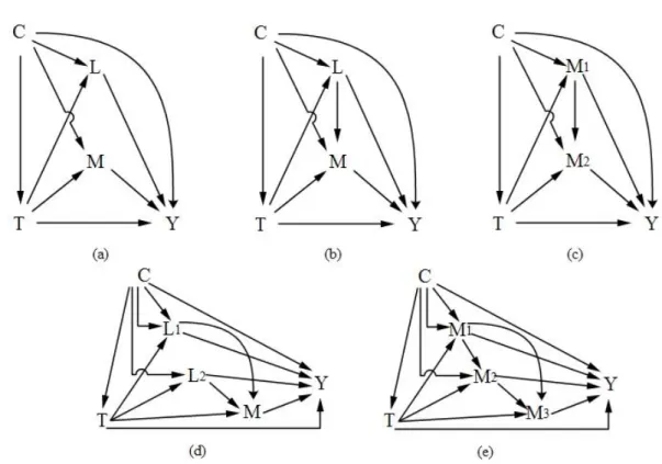
FIGURE 1 COMES SOMEWHERE HERE
When mediators are causally independent of one another (i.e., parallel or non-intertwined) the same analytical strategy can be pursued as with a single mediator. Notably, this causal independence is an untestable assumption that makes it difficult to assess whether Figure1 (a) or (b) is more suitable for the constructs analysed. Nonetheless, an obvious way of examining the potential dependence between variables is to regress T, C, and L on the M of interest. Significant relationships can provide a reasonable indication that the variables are dependent on each other (Imai & Yamamoto, 2013). However, even if no statistically significant association emerges, it is usually difficult to argue for the orthogonality of the mediators, unless there is a convincing theoretical reason to do so, or such orthogonality is artificially created (e.g., through varimax rotation in exploratory factor analysis). A rare example of such independence was provided by Taguri, Featherstone, and Cheng (2018), who examined two unrelated techniques to prevent dental cavities, through antibacterial and fluoride therapy mediators. Nevertheless, it is usually difficult to encounter such clear-cut cases in the social
12
sciences. Finally, assessing the mediators one at a time will also fail if there are interactions between the effects of the various mediators on the outcome (Lange, Rasmussen, and Thygesen 2014).
Assuming causal dependence between L and M, a simple solution is to examine their joint effect and treat them as a vector of mediators (Steen et al. 2017b; VanderWeele and Vansteelandt 2014). Importantly, L and M are statistically equivalent, the post-treatment confounder label of L is only substantive, hence, L can be considered as a second mediator. Handling multiple mediators as a single vector is robust to unmeasured common causes of various mediators, and can even accommodate cases with causal ordering of M1 and M2 similar
to Figure1 (c). Crucially, the sequential ignorability assumption (i-iv) is still valid, but now for a vector of mediators instead of a single mediator. Admittedly, this approach limits the scope of the analysis, yet it can be pragmatic for certain research questions (e.g., if we are only interested in the mediated effects of legitimacy as a whole on the outcome of interest). Even so, for many applied cases this technique will remain untenable. For instance, it would be hard to justify this approach in Rivera and Tilcsik’s (2016) study where the commitment and fit for a job are fairly different aspects. Similarly, this strategy would not allow one to test the unique impact of moral alignment with the police and duty to obey the police. In such circumstances, assuming causal mediation analysis with post-treatment confounders or sequentially ordered mediators need to be considered, which will be discussed in the next two sections.
Causal mediation analysis with post-treatment confounding
Avin, Shpitser, and Pearl (2005) in their proof showed that conditioning on L does not permit the non-parametric identification of natural effects, but only the CDEs (for which assumption (i) and (ii) are sufficient enough). The biggest issue in the presence of causally dependent L is that testing the mediators one at a time will no longer be viable because this results in counting certain causal pathways more than once (VanderWeele and Vansteelandt
13
2014). A further problem emphasised by some (Daniel, De Stavola, and Cousens 2011) is that the direct effect of T on Y will not estimate consistently if there is an uncontrolled post-treatment confounder L that opens a backdoor path of T → L → Y. A seemingly easy fix to this problem is to condition for L as well. However, since L was affected by T controlling for L in the model for M, this blocks the T → L → Y path, which will also result in biased estimates for the NDE and NIE5.This means that neither the inclusion nor the exclusion of L will solve the problem of identifiability.
Thus, to address these issues we require a refined – and relaxed – sequential ignorability assumption to make the NIE and NDE identifiable. Crucially, these alternatives do not contradict Avin et al. (2005), but introduce additional assumptions to make the natural effects estimable. While several alternative sets of identifiability criteria have been established (Tchetgen Tchetgen and VanderWeele 2014), the one postulated by De Stavola et al. (2015) will be discussed here. De Stavola et al. (2015) modified the definition of Imai and Yamamoto (2013), positing that sequential ignorability in the presence of post-treatment confounder L holds when controlling for pre-treatment covariates C when there is:
v. No unmeasured confounding of the T-Y, T-M, and T-L relationship or (Ytml Mtl Lt)╨T|C
vi. No unmeasured confounding of the M-Y relationship also controlling for T and L or Ytml╨M|C, T, L
vii. No unmeasured confounding of the L-Y relationship also controlling for T or Ytl╨L|C,
T
viii. No unmeasured M-Y confounder Z that was affected by T or Ytm╨Mt*|C, L
These assumptions are analogous to (i-iv). Assumption (v) is satisfied in the case of a random assignment of T, while (vi) makes the mediated effect conditional on L. Assumption (vii) stresses that there cannot be any unmeasured confounder for the L-Y relationship, which is again a strong assumption similar to (ii). Finally, (viii) establishes that there cannot be any
14
post-treatment confounder Z that was not included in L (i.e., all post-treatment confounders – in other words, alternative mediators – are measured).
Under assumptions (v-vii) the NDE and NIE are identifiable with a few additional limitations. Firstly, the analyst needs to rely on the linearity assumption, which permits the additivity of the effects. Secondly, it needs to be assumed that there is no significant T-M interaction for Y (Robins and Greenland 1992) or that both the T-L interaction and L2 are zero in the model for Y (Petersen, Sinisi, and van der Laan 2006). Importantly, this second modelling assumption is a loosened version of SEM’s effect homogeneity assumption that only needs to be true on average, not for each individual, thus it can be empirically assessed (Imai and Yamamoto 2013). Crucially, and as demonstrated by De Stavola et al. (2015), when these parametric assumptions are met, (vii) is automatically satisfied.
Provided that the model is identifiable, a generalised structural equation model needs to be specified with L modelled on C and T, M modelled on C, T, and L, and Y modelled on C, T, L, and M. In addition, the interaction between T and L is entered in the model for both M and Y, and the squared transformation of M and L in the model for Y to control for potential quadratic and heterogeneous effects in line with the earlier identification assumptions6. Then, a generalised version of the product method is used to obtain the parameters. G-computation of the causal estimates for NDE and NIE can be accomplished by combining these appropriate parameters from the SEM through estimation by combination. Unfortunately, with more complex models this mathematical integration can become exceedingly cumbersome with potential issues of convergence. To overcome this difficulty, Monte Carlo simulation is used as a more flexible and efficient way to approximate the integration, whilst the standard errors and confidence intervals are bootstrapped (Daniel et al. 2011). As acknowledged by De Stavola et al. (2015), the results of this approach will coincide with a traditional SEM, provided that there
15
are no interactions or nonlinear terms of M, L, or T (for the equations discussed in this paragraph please refer to Appendix/C).
Finally, it is crucial to assess the robustness of the M-Y relationship to potential unmeasured confounding. De Stavola et al. (2015) devised a sensitivity analysis based on Imai et al.'s (2011) method that can be applied in the presence of post-treatment confounders. This refined method fits a SEM which allows for the error terms of the models for Y and M to become correlated7. These error terms are very instructive as they incorporate the impact of the unmeasured confounders. This method regresses L on X and C, M on L, X, and C, and Y on X, L, and C. M is not included in the model for Y as to do so would induce collinearity. Then the error terms from the model for M and Y are systematically correlated, where ρ’ provides an indication of how big the correlation must be between the two error terms to make the M-Y relationship zero. A confidence interval for ρ’ can also be obtained with bootstrapping.
Preliminary remarks
Confirmatory factor analysis was used to derive factor scores for the respective constructs in both studies. These factor scores were entered in the causal mediation analysis. Although this strategy might have resulted in increased measurement error bias compared to using latent variables to capture multiple indicators (Loeys et al. 2014), the reliance on latent variables, their interactions and transformations (i.e., squared-forms) would have added to the computational complexity and prolonged the already fairly long estimation time. Moreover, the concepts and definitions of causal effects only apply to the structural model, not the measurement models. Thus for pragmatic reasons, factor scores were used instead of latent variables to demonstrate the use of causal mediation analysis with multiple mediators.
All analyses in this paper were carried out using STATA 14 and its multicore (MP) version with g-computation models relying on 100,000 Monte Carlo simulations and the number of bootstraps set to 300. The cap on the number of bootstraps was placed so that the analysis would
16
mirror a realistic application, as causal mediation analysis with post-treatment confounding can be particularly time-consuming. With the current specification it takes five days with a regular office computer and a single core, and two days with a cluster computer and six cores to obtain results. The estimation of causal mediation analysis with sequentially ordered mediators is speedier, taking a matter of minutes.
TABLE 1 COMES SOMEWHERE HERE Test of identification
Two linear regression analyses were fitted for cooperation for the two studies. In both cases the treatment, the covariates (gender, age, ethnic minority background) and the two potential mediators, their quadratic transformation, and their interaction with the treatment were included (Table 1). As discussed earlier, including these additional parameters in the regression models for the respective Y and examining their significance helps in determining which identification strategy – if any – is relevant for a particular model. However, as noted by VanderWeele (VanderWeele 2015; VanderWeele and Knol 2014), strong statistical power is usually needed to discover interactions, therefore it is worth also examining effect sizes, especially with smaller sample sizes. In this paper, the sample sizes are moderate and the effect sizes are relatively uneqivocal, which means that considering the statistically significant effects should be sufficient.
For Study 1 either identification strategy (Petersen et al. 2006; Robins and Greenland 1992) should suffice as neither the interactions, nor the quadratic terms are significant. However, for the second study, neither will be appropriate, as there are moderately strong and significant interactions between the treatment and both mediators. The NDE and NIE can still be estimated, but they have no meaningful interpretation, thus they are not included in the results table (Table 2). Nevertheless, the TE is always estimable, as well as the CDE(m), provided that assumptions (v) and (vi) are satisfied.
17 Results for causally dependent mediators
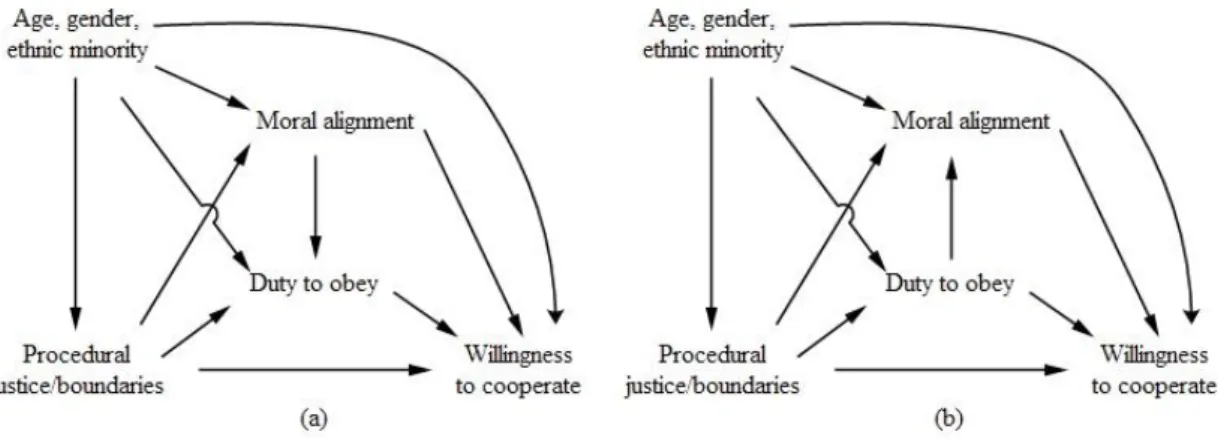
As discussed earlier, some scholars (e.g., Hough et al. 2013) believe that the two aspects of legitimacy, moral alignment and duty to obey, mutually reinforce each other. In the SEM literature this is depicted using a bidirectional arrow that denotes a correlation between the constructs. By contrast, the causal inference literature utilises directed acyclic graphs (DAGs), which do not allow two-headed arrows as to do so would create a cycle. Hence, when mutual reinforcement is hypothesised two graphs are created for the two different causal directions (Figure 2 (a) and (b)).
FIGURE 2 COMES SOMEWHERE HERE
In causal mediation analysis with post-treatment confounding the NIE incorporates the mediated effect of the mediator of interest (including L’s impact on M) and the NDE the effect of the treatment not going through M (including L’s impact on Y). In Study 1 (Table 2) procedural justice treatment has a significant positive effect (NDE=0.254, p<0.01) and a significant mediated effect through moral alignment with the police (NIE=0.215, p<0.001), which carries approximately 46% of the total effect. The sensitivity analysis indicates that on average a relatively strong correlation of ρ’=0.42 would be needed between the error terms to nullify the mediated effect with a 95% confidence interval of 0.301 and 0.545. Conversely, duty to obey the police has a weak non-significant impact on cooperation (NIE=0.043, p>0.05) and transmits only 9% of the total effect. The sensitivity analysis implies that on average a ρ’=0.199 between the error terms could make the impact non-significant, but the confidence intervals show that a correlation of 0.047 might be enough to make the effect zero. Procedural justice has a strong and significant direct effect on willingness to cooperate (NDE=0.423, p<0.001). The estimates of CDE(m) and NDE are both within rounding error of each other in both cases, which is unsurprising given the absence of a treatment-mediator interaction, in which case they should approximately coincide (i.e., as a default the CDE’s m is always set at the average value
18
of the mediator, as this option allows the comparison to the NIE). Overall, it seems that moral alignment with the police has a fairly strong causally mediated effect on cooperation with the police, while duty to obey does not seem to have an impact. Receiving the procedural justice treatment also significantly increased the participants’ willingness to cooperate with the police.
TABLE 2 COMES SOMEHWERE HERE
For Study 2, only the CDE(m) and TCE were identifiable. For both moral alignment (CDE(m)=1.276, p<0.001) and duty to obey (CDE(m)=1.763, p<0.001) as mediators the controlled direct effect of legality was significant. Unfortunately, CDE(m) does not permit effect decomposition, thus no information can be gained regarding the mediated effects. Still, the CDE(m) was much higher than in Study 2, which implies that legal police practices might have an even stronger effect when the police are otherwise thought to overstep legal boundaries. Causal mediation analysis with sequentially ordered mediators
Interdependence between mediators can take the form of a causal chain where the first mediator affects the second mediator and the outcome, but not the other way around. Crucially, this situation’s DAG takes the very same form as the post-treatment confounder case’s as shown in Figure 1 (b) and (c) where the difference between the two graphs is only substantive. The distinction between the two approaches becomes clearer looking at Figure 1 (d) and (e), which show that in the post-treatment confounder case L1 and L2 do not affect one another, while in
the sequential case M1 and M2 do, following a pre-determined order. This difference in the
causal structure leads to an alternative four-way decomposition in case of two mediators where there will be NIE1 standing for M1’s mediated effect on Y (T→M1→Y), NIE2 for M2’s mediated
effect on Y (T→M2→Y), NIE12 for M1’s and M2’s jointly mediated effect on Y
(T→M1→M2→Y), and NDE, T’s effect that does not go through either of the mediators
(T→Y). Although there have been other approaches addressing causally ordered mediators (Steen et al. 2017a, 2017b), Daniel et al. (2015) has been the only paper so far to allow for this
19
finest four-way decomposition. As before, this new decomposition will require a modified set of sequential ignorability assumptions; controlling for pre-treatment covariates C, these are:
ix. No unmeasured confounding of the T-Y, T-M1, and T-M2 relationship or
(Ytm1m2 M2tm1 M1t)╨T|C
x. No unmeasured confounding of the M1-Y relationship also controlling for T or
Ytm1m2╨M1|C, T
xi. No unmeasured confounding of the M2-Y relationship also controlling for T and M1 or
Ytm1m2╨M2|C, T, M1
xii. No unmeasured M1-Y, M1-M2 or M2-Y confounder L1 or L2 that was affected by T or
Ytm1m2╨M1t*|C, M2tm1╨ M1t*|C, and Ytm1m2╨M2t**|C, M1t*
When T is randomly assigned, (ix) will automatically be satisfied. (x) is analogous to (ii) and (xi) to (vi), while (xii) states again that there cannot be post-treatment confounders L1 or
L2 that were affected by the treatment. As with the post-treatment confounder case, certain
parametric restrictions are also needed. As earlier, the linearity assumption is required so the additivity of the effects is guaranteed. Furthermore, when M1 has a non-zero effect on M2 the
conditional correlation between M1’s potential outcomes is required to make the effects estimable. However, this conditional correlation is unknown for several of the effects8, hence a sensitivity parameter κ2 is used, which stands for the proportion of residual variance shared across the two hypothetical worlds. κ2can take values from 0 to 1, where 0 means no correlation
between the potential outcomes conditional on C, and 1 means perfect correlation between the potential outcomes conditional on C (Daniel et al. 2015).
Because of the second mediator, the conditional expectations take more complex forms: generally they are E[Y(t,M1(t*),M2(t**,M1(t***)))], where the different t-s (i.e., t, t*, t**, t***) stand
for setting the treatment to one of its possible values. This increased complexity also means that the number of possible decompositions of the total effect will be (2n)!, where n stands for the
20
number of mediators. In the case of two mediators, the 24 (i.e., (22)!=(4)!=(4x3x2x1)=24) possible decompositions are reduced to 6 when M1 does not affect M2. Overall, marked
differences among the path-specific effects only emerge when there are significantM1 and T-M2 interactions, which are allowed with the current technique. In the absence of interactions, the estimates will be approximately the same as SEM’s estimates, albeit with wider confidence intervals (Daniel et al. 2015).
Because interpreting a high number of estimates from the different decompositions can be cumbersome, and usually not of particular interest, it is worth considering ways to summarise the effects. Based on earlier work (Kuha and Goldthorpe 2010), Daniel et al. (2015) recommended the usage of summary effects that are weighted averages of the NDE and various NIEs. In addition, they also advised reporting the variance estimates for these summary effects, which indicate whether there are large differences across the various decompositions. The major advantage of these summary effects is that they provide a good approximation of the respective effects, however it is hard to attach a substantive interpretation, which can prove problematic especially if the particular effect size on the outcome variable were directly interpretable and of particular interest.
Results for sequentially ordered mediators
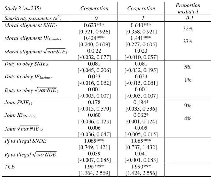
In the procedural justice literature, other scholars (e.g., Huq, Jackson, & Trinkner 2017) have argued for the theoretical model depicted by Figure 2 (b), where duty to obey the police is influenced by moral alignment with the police, but not the other way around. The results (Tables 3-4) are presented conditionally only on the two extremes of the sensitivity value (κ2=0 and κ2=1), as they appear to be mostly robust to these extremes. In the case of wider disparities,
it is advisable to look at further values of the sensitivity parameter. TABLE 3 COMES SOMEWHERE HERE
21
The results from Study 1 (Table 3, Appendix Figure 3-6) show that moral alignment with the police has a moderately strong mediated effect (SNIE1κ2=0=0.231, p<0.01, SNIE1κ2=1=0.219,
p<0.01) on willingness to cooperate with the police with 42-46% of the effect transmitted by it. In contrast, duty to obey does not have an impact on any conventional level of statistical significance (SNIE2κ2=0=-0.01, p>0.05, SNIE2κ2=1=-0.009, p>0.05). The joint effect of moral
alignment with and duty to obey the police has a weak significant relationship with willingness to cooperate when κ2=0 (SNIE
12κ2=0=0.061, p<0.05), but it does not reach the 5% significance
level when κ2=1 (SNIE12κ2=1=0.038 p>0.05). Procedural justice treatment has a moderately
strong effect on cooperation, but it does not reach statistical significance (SNDEκ2=0=0.218, p>0.05, SNDEκ2=1=0.273, p>0.05). Juxtaposing the results of the two extremes of the sensitivity parameter shows that when the counterfactual outcomes of M1 are assumed to be perfectly
correlated, it slightly boosts the SNDE and widens its confidence intervals but at the same time reduces the mediated effects and narrows their confidence intervals. The variance estimates are tiny across the different effects, which is in accordance with the lack of interactions found earlier (Table 1). The absence of interactions also means that the indirect effects (IEs) from an SEM should be very close to the SNIEs which, as expected, they are.
The findings from Study 1 seem to uphold moral alignment’s moderately strong mediated effect on willingness to cooperate while also confirming the lack of impact from duty to obey. The joint effect of the two mediators is either weak or non-existent while the direct effect of procedural justice does not reach statistical significance; a bigger sample size would be needed to elucidate the treatment’s and the joint effect’s impact on the outcome.
The results from Study 2 (Table 4, Appendix Figure 7-10) show a similar pattern to Study 1. Moral alignment with the police has a strong mediated effect (SNIE1κ2=0=0.623, p<0.001,
SNIE1κ2=1=0.640, p<0.001) with 32% proportion mediated while duty to obey has a weak
22
mediated effect is either significant (SNIE12κ2=1=0.184, p<0.05) or not (SNIE12κ2=0=0.178,
p>0.05), depending on the value taken by the sensitivity parameter. The direct effect of legality is much stronger in Study 2 than procedural justice’s in Study 1 with a statistically significant impact (SNDEκ2=0=1.085, p<0.001, SNDEκ2=1=1.085, p<0.001). The results are even less sensitive to changes in κ2 than in Study 1, and the perfect correlation between the potential
outcomes of M1 here increases the effect sizes while decreasing the confidence intervals for all
effects. The variance estimates are much higher than in Study 1, which is expected because of the interaction effects (Table 1). This also means that indirect effects conventionally obtained from an SEM will be different: in this case they are much smaller than the ones from causal mediation analysis.
TABLE 4 COMES SOMEWHERE HERE
Overall the results provide further support for the earlier findings. From the two components of legitimacy shared values (moral alignment) appears to be the important mediator of legality’s impact on cooperation while consent (duty to obey) does not seem to matter much. The joint effect of these two elements is very close to zero and requires further scrutiny. The strong direct effect indicates that procedurally just and legal messaging will have a powerful impact, especially when compared to the assumption that the police routinely overstep their boundaries.
In summary, both the post-treatment confounder and sequentially ordered approach concur that moral alignment is the primary conduit of the effect of procedural justice and legality on willingness to cooperate, while duty to obey either does not have an effect or has only a weak joint one with moral alignment. The direct effect of the two treatment conditions also seemed to be important, even if not consistently significant between the two methods. These results are in line with earlier research (e.g., Moravcová 2016; Tyler & Jackson 2014), which found a small or even non-significant relationship between duty to obey and cooperation, and which thus
23
called into question its relevance. As with other experiments, the external validity of the results is limited and further studies are needed to attest to the effects found here.
TABLE 5 COMES SOMEWHERE HERE Discussion
Over the last couple of decades, many social science disciplines have relied primarily on SEM (and path analytical models more generally) for assessing complex theories. Yet, adopting the potential outcome framework provides at least three advantages (Daniel, Stavola, and Vansteelandt 2016; Greenland 2017; Steen et al. 2017a):
• it makes explicit the identification assumptions needed to avoid model misspecification for the mediator(s);
• it provides formal definitions of the estimated causal effects; and,
• it devises ways to check for the robustness of the results through sensitivity analysis of certain causal identification assumptions9.
This paper has argued that the traditional SEM framework has shortcomings that need to be addressed for more realistic identification and effect decomposition. In order to accommodate multiple mediated effects, parametric restrictions akin to SEM need to be made: linearity and relaxed effect homogeneity for the post-treatment confounder, and linearity for the causally ordered case (for a summary see Table 5). The similarity between the two approaches does not end there; traditional SEM can be considered a special case of causal mediation analysis when certain conditions apply. This means that SEM and causal mediation analysis can be easily reconciled, and that the estimation method will be very similar to each other, which makes such techniques easily understandable and adaptable for those who were primarily trained for SEM (Daniel et al. 2015; De Stavola et al. 2015).
Study 1 and Study 2 exemplify how SEM compares to causal mediation analysis with multiple mediators. The results from Study 1 were approximately identical to the results one
24
would have derived using SEM. In contrast, for Study 2 the post-treatment confounder case was not identifiable, while the sequentially ordered mediator case differed decidedly from the SEM results. Study 1 highlights how traditional SEM can sometimes hit the mark, while Study 2 illustrates that it can also fail. The sensitivity analysis from the different studies can help to determine whether the results are robust to certain conditions (unmeasured confounding or the correlation of certain potential outcomes). The reliance on these sensitivity measures can mitigate bad practices, like “p-hacking” and can help to identify spurious relationships and statistical flukes. This perspective also encourages researchers to adapt a priori model building since their decision will have a major impact on the modelling strategy employed, and because the causal structure can never be decided by relying on statistical methods.
Nevertheless, there are certain limitations worthy of discussion. First, causal mediation analysis relies on very strong assumptions. Even in the case of a randomly assigned treatment, the M-Y relationship can be spurious unless a proper set of covariates is controlled for. In Study 1 and Study 2 only three covariates (age, gender, and ethnic minority background) were considered, which are far from being sufficient (Steiner et al. 2010). The problem of no unmeasured confounding is further aggravated in observational studies where the treatment is not randomised. Some scholars have recommended conducting ‘comprehensive SEM’ (Mackinnon and Pirlott 2015) with up to fifty covariates, yet even in such cases it can be difficult to realistically argue for causal inference. Multiple mediators can even exacerbate this issue as it is more likely that at least one of them is affected by unmeasured confounding (VanderWeele 2015).
As an alternative to natural effects, some have recommended the use of interventional effects (Vansteelandt and Daniel 2017), which require weaker causal identifying assumptions. However, these loosened assumptions posit additional parametric restrictions to the ones that have been discussed in this paper (e.g., fixing the mediator distribution). Arguably, these
25
alternatives can sometimes be more policy relevant (i.e., the interventional indirect effects are set at the levels of the potential interventions), but they provide less information regarding the causal mechanisms and hence are often times less generalisable to other contexts.
Others are also critical of SEMs because of their restrictive parametric assumptions, which were (partially) adopted for causal mediation analysis in the current applications. VanderWeele has repeatedly insisted (VanderWeele 2012, 2015, 2016) that these modelling assumptions are too strong, and SEMs and similar methods should only be used for hypothesis generation not hypothesis testing. In addition, both Keele (2015a) and Kennedy (2015) have argued that because causal effects are non-parametrically identified, parametric models are more likely to yield misspecification and the use of semi- or non-parametric models is more advisable. Although such alternatives are available for multiple mediators (Kim, Daniels, and Hogan 2017; Moerkerke, Loeys, and Vansteelandt 2015; Tchetgen Tchetgen and VanderWeele 2014), they have other restrictions and limitations (e.g., particular types of outcome, constrained effect decomposition, Bayesian model-specification) that make them unappealing or hard to implement.
Even if these criticisms are valid, most of the propositions made in this paper touch upon the fundamental limitations of SEM and can be considered as improvements upon it. For instance, the no-interaction assumption is a non-causal issue, yet applying a causal mediation perspective helps to address the matter. Similarly, the current methods allow to incorporate quadratic terms in the model, provide an alternative way to investigate cases when mediators are assumed to mutually reinforce each other, and propose sensitivity analysis for model assessment. In the end, causal mediation analysis provides a list to consider for causal analysis, a slightly modified estimation approach that allows for a more versatile model analysis and assessment, and provides a comprehensive improvement upon the traditional SEM.
26 Bibliography
Avin, C., Shpitser, I., & Pearl, J. (2005). Identifiability of path-specific effects. Proceedings of the international joint conferences on artifical intelligence, 34, 163–192.
Baron, R. M., & Kenny, D. A. (1986). Moderator-Mediator Variable Distinction in Social Psychological Research: Conceptual, Strategic, and Statistical Considerations. Journal of Personality and Social Psychology, 51(6), 173–182.
Bentler, P. M., & Chou, C. P. (1987). Practical issues in structural modeling. Sociological methods and research. 16(1), 78-117.
Bollen, K. A., & Pearl, J. (2013). Eight Myths About Causality and Structural Equation Models. In S. L. Morgan (Ed.), Handbook of Causal Analysis for Social Research (pp. 301–328). Springer.
Bradford, B. (2014). Policing and social identity: procedural justice, inclusion and cooperation between police and public. Policing and Society, 24(1), 22–43.
Bradford, B., Stanko, E., & Jackson, J. (2012). Just Authority? - Trust in the Police in England and Wales. Routledge.
Browne, M. W., & Cudeck, R. (1992). Alternative ways of assessing model fit. Sociological methods & research, 21(2), 230-258.
Coffman, D. L., & Zhong, W. (2012). Assessing Mediation Using Marginal Structural Models in the Presence of Confounding and Moderation. Psychological Methods, 17(4), 642–664. Daniel, R. M., De Stavola, B. L., & Cousens, S. N. (2011). gformula - Estimating causal
effects in the presence of time-varying confounding or mediation using the g-computation formula. The Stata Journal, 11(4), 479–517.
Daniel, R. M., De Stavola, B. L., Cousens, S. N., & Vansteelandt, S. (2015). Causal mediation analysis with multiple mediators. Biometrics, 71(1), 1–14.
27
quantitative causal inference in epidemiology: misguided or misrepresented? International Journal of Epidemiology, (section 2), 1–14.
De Stavola, B. L., Daniel, R. M., Ploubidis, G. B., & Micali, N. (2015). Mediation analysis with intermediate confounding: Structural equation modeling viewed through the causal inference lens. American Journal of Epidemiology, 181(1), 64–80.
Greenland, S. (2017). For and Against Methodologies: Some Perspectives on Recent Causal and Statistical Inference Debates. European Journal of Epidemiology, 32(1), 1–18. Hough, M., Jackson, J., & Bradford, B. (2013). Legitimacy, Trust and Compliance: An
Empirical Test of Procedural Justice Theory Using the European Social Survey. In J. Tankebe & A. Liebling (Eds.), Legitimacy and Criminal Justice - An International Exploration (pp. 326–353). Oxford University Press.
Huq, A. Z. A. H., Jackson, J., & Trinkner, R. J. (2017). Legitimating practices: Revisiting the predicates of police legitimacy. British Journal of Criminology, (57), 1101–1122.
Imai, K., Keele, L., & Tingley, D. (2010). A general approach to causal mediation analysis. Psychological methods, 15(4), 309–34.
Imai, K., Keele, L., Tingley, D., & Yamamoto, T. (2011). Unpacking the black box of
causality: Learning about causal mechanisms from experimental and observational studies. American Political Science Review, 105(4), 765–789.
Imai, K., Keele, L., & Yamamoto, T. (2010). Identification, Inference and Sensitivity Analysis for Causal Mediation Effects. Statistical Science, 25(1), 51–71.
Imai, K., Tingley, D., & Yamamoto, T. (2013). Experimental Designs for Identifying Causal Mechanisms (with {D}iscussion). J. Roy. Stat. Soc., A, 176, 5–51.
Imai, K., & Yamamoto, T. (2013). Identification and sensitivity analysis for multiple causal mechanisms: Revisiting evidence from framing experiments. Political Analysis, 21(2), 141–171.
28
Jackson, J., Bradford, B., Hough, M., Myhill, A., Quinton, P., & Tyler, T. R. (2012). Why do people comply with the law? British Journal of Criminology, 52(6), 1051–1071.
Jo, B. (2008). Causal Inference in Randomized Experiments With Mediational Processes. Psychological Methods, 13(4), 314–336.
Judd, C. M., & Kenny, D. A. (1981). Estimating the effects of social interventions. Camdridge University Press.
Kaplan, D. (2008). Structural Equation Modeling - Foundations and Extensions (2nd ed.). SAGE.
Keele, L. (2015a). The statistics of causal inference: A view from political methodology. Political Analysis, 23(3), 313–335.
Keele, L. (2015b). Causal Mediation Analysis Warning! Assumptions Ahead. American Journal of Evaluation, 46(4), 500–513.
Kennedy, E. H. (2015). Semiparametric theory and empirical processes in causal inference, 1– 26.
Kenny, D. A. (2008). Reflections on Mediation. Organizational Research Methods, 11(2), 353–358.
Kim, C., Daniels, M. J., & Hogan, J. W. (2017). Bayesian Methods for Multiple Mediators : Relating Principal Stratification and Causal Mediation in the Analysis of Power Plant Emission Controls, 1–36 https://dataverse.harvard.edu/dataverse.xhtml?alias=mmediators. Kline, R. B. (2015). The mediation myth. Basic and Applied Social Psychology, 37(4), 202–
213.
Kuha, J., & Goldthorpe, J. H. (2010). Path analysis for discrete variables: the role of
education in social mobility. Journal of the Royal Statistical Society Series a-Statistics in Society, 173, 351–369.
29
effects through multiple pathways. American Journal of Epidemiology, 179(4), 513–518. Liu, P., Chen, J., Lu, Z., & Song, X. (2014). Transformation Structural Equation Models With
Highly Nonnormal and Incomplete Data. Structural Equation Modeling: A Multidisciplinary Journal, 5511(ahead-of-print), 1–15.
Loeys, T., Moerkerke, B., Raes, A., Rosseel, Y., & Vansteelandt, S. (2014). Estimation of Controlled Direct Effects in the Presence of Exposure-Induced Confounding and Latent Variables. Structural Equation Modeling, 21(3), 396–407.
Mackinnon, D. P. (2008). Introduction to Statistical Mediation. Erlbaum.
Mackinnon, D. P., Kisbu-sakarya, Y., & Gottschall, A. C. (2013). Developments in Mediation Analysis Oxford Handbooks Online Developments in Mediation Analysis. In T. D. Little (Ed.), Oxford Handbook of Quantitative Methods (Volume 2., Vol. 2, pp. 1–28). New York: Oxford University Press.
Mackinnon, D. P., & Pirlott, A. G. (2015). Statistical Approaches for Enhancing Causal Interpretation of the M to Y Relation in Mediation Analysis. Personality and Social Psychology Review, 19(1), 30–43.
Manski, C. F. (2007). Identification for Prediction and Decision. Harvard University Press. Mauro, R. (1990). Understanding L.O.V.E. (Left Out Variable Error): A Method for
Estimating the Effects of Omitted Variables, 108(2), 314–329.
Mayer, A., Umbach, N., Flunger, B., & Kelava, A. (2017). Effect Analysis Using Nonlinear Structural Equation Mixture Modeling. Structural Equation Modeling: A Multidisciplinary Journal, 24(4), 556–570.
Mazerolle, L., Antrobus, E., Bennett, S., & Tyler, T. R. (2013). Shaping Citizen Perceptions of Police Legitimacy: A Randomized Field Trial of Procedural Justice. Criminology, 51(1), 33–63.
30
marginal structural modeling for assessing mediation in the presence of posttreatment confounding. Psychological Methods, 20(2), 204–220.
Pearl, J. (2001). Direct and indirect effects. Proceedings of the Seventeenth Conference on Uncertainty in Artificial Intelligence UAI’01, (1992), 411–420.
Pearl, J. (2010). On the consistency rule in causal inference: axiom, definition, assumption, or theorem? Epidemiology, 21(6), 872–875.
Pearl, J. (2014). Interpretation and Identification of Causal Mediation. Psychological methods, 19(4), 459–481.
Pek, J., & MacCallum, R.C. (2011). Sensitivity Analysis in Structural Equation Models: Cases and Their Influence. Multivariate Behavioral Research, 46, 202-228.
Petersen, M. L., Sinisi, S. E., & van der Laan, M. J. (2006). Estimation of Direct Causal Effects. Epidemiology, 17(3), 276–284.
Pirlott, A. G., & Mackinnon, D. P. (2016). Design approaches to experimental mediation. Journal of Experimental Social Psychology, 66, 29–38.
Preacher, K. J. (2015). Advances in mediation analysis: a survey and synthesis of new developments. Annual review of psychology, 66, 825–52.
Rivera, L. A., & Tilcsik, A. (2016). Class Advantage, Commitment Penalty: The Gendered Effect of Social Class Signals in an Elite Labor Market. American Sociological Review, 1– 68.
Robins, J. M., & Greenland, S. (1992). Identifiability and Exchangeability for Direct and Indirect Effects. Epidemiology, 3(2), 143–155.
Sardeshmukh, S. R., & Vandenberg, R. J. (2016). Integrating Moderation and Mediation : A Structural Equation Modeling Approach, 1–25.
Shadish, W. R., Cook, T. D., & Campbell, D. T. (2002). Experimental and Quasi-Experimental Design for Generalized Causal Inference. Houghton Mifflin Company.
31
Steen, J., Loeys, T., Moerkerke, B., & Steen, J. (2017a). Flexible mediation analysis with multiple mediators. American Journal of Epidemiology. 186(2), 184-193.
Steen, J., Loeys, T., Moerkerke, B., & Vansteelandt, S. (2017b). Medflex : An R Package for Flexible Mediation Analysis using Natural Effect Models. Journal of Statistical Software, 76(11), 1–45.
Steiner, P. M., Cook, T. D., Shadish, W. R., & Clark, M. H. (2010). The Importance of Covariate Selection in Controlling for Selection Bias in Observational Studies, 15(3), 250– 267.
Taguri, M., Featherstone, J., & Cheng, J. (2018). Causal mediation analysis with multiple causally non-ordered mediators. Statistical Methods in Medical Research, 27(1), 3–19. Tchetgen Tchetgen, E. J., & VanderWeele, T. J. (2014). Identification of natural direct effects
when a confounder of the mediator is directly affected by exposure. Epidemiology., 25(2), 282–291.
Tomarken, A. J., & Waller, N. G. (2005). Structural Equation Modeling: Strengths,
Limitations, And Misconceptions. Annual Review of Clinical Psychology. Vol 1(1), 31–65. Trinkner, R., Jackson, J., & Tyler, T. R. (2017). Expanding “Appropriate” Police Behavior
Beyond Procedural Justice - Bounded Authority. osf.io/preprints/socarxiv/nezm6
Tyler, T., & Fagan, J. (2006). Legitimacy and Cooperation: Why Do People Help the Police Fight Crime in Their Communities? Ohio State Journal of Criminal Law, 6, 231–275. Tyler, T. R. (2006). Why people obey the law. Princeton: Princeton University Press.
Tyler, T. R., Goff, P. A., & MacCoun, R. J. (2015). The Impact of Psychological Science on Policing in the United States: Procedural Justice, Legitimacy, and Effective Law
Enforcement. Psychological Science in the Public Interest (Vol. 16). !!!
Tyler, T. R., & Jackson, J. (2013). Future Challenges in the Study of Legitimacy and Criminal Justice. In J. Tankebe & A. Liebling (Eds.), Legitimacy and Criminal Justice - An
32 International Exploration (pp. 83–104). Wiley.
Tyler, T. R., & Jackson, J. (2014). Popular legitimacy and the exercise of legal authority: Motivating compliance, cooperation, and engagement. Psychology, Public Policy, and Law, 20(1), 78–95.
VanderWeele, T. J. (2012). Invited commentary: Structural equation models and epidemiologic analysis. American Journal of Epidemiology, 176(7), 608–612.
VanderWeele, T. J. (2015). Explanation in Causal Inference - Methods for Mediation and Interaction. Oxford University Press.
VanderWeele, T. J. (2016). Mediation Analysis: A Practitioner’s Guide. Annual Review of Public Health, 37(1), 17–32.
VanderWeele, T. J., & Knol, M. J. (2014). A Tutorial on Interaction. Epidemiological Methods, 3(1), 33–72.
VanderWeele, T. J., & Vansteelandt, S. (2014). Mediation Analysis with Multiple Mediators. Epidemiologic Methods, 2(1), 95–115.
Vansteelandt, S., & Daniel, R. M. (2017). Interventional effects for mediation analysis with multiple mediators. Epidemiology, 28(2), 258–265.
Wang, A., & Arah, O. A. (2015). G-computation demonstration in causal mediation analysis. European Journal of Epidemiology, 30(10), 1119–1127.
Westreich, D., Edwards, J. K., Cole, S. R., Platt, R. W., Mumford, S. L., & Schisterman, E. F. (2015). Imputation approaches for potential outcomes in causal inference. International Journal of Epidemiology, (July), 1731–1737.
White, M. D., Mulvey, P., & Dario, L. M. (2016). Arrestees’ Perceptions of the Police. Criminal Justice and Behavior, 43(3), 343–364.
33 Tables Study 1 Study 2 Moral alignment 0.368*** [0.193, 0.544] 1.143*** [0.703, 1.583] Moral alignment2 -0.044 [-0.144, 0.056] 0.120 [-0.018, 0.257]
Moral al. X Treatment -0.037
[-0.248, 0.174] -0.478*** [-0.699, -0.257] Duty to obey 0.193* [0.014, 0.373] 0.570* [0.087, 1.107] Duty to obey2 -0.006 [-0.101, 0.089] 0.059 [-0.075, 0.194]
Duty to obey X Treatment -0.097
[-0.324, 0.130] -0.365** [-0.647, -0.083] Treatment 0.282** [0.0822, 0.483] 1.136*** [1.067, 1.648] Gender 0.096 [-0.051, 0.243] 0.117 [-0.017, 0.252] Age (years) -0.003 [-0.051, 0.243] -0.006* [-0.012, -0.001] Ethnic minority -0.207* [-0.374, -0.040] -0.111 [-0.300, 0.077] Constant 0.014 [-0.365, 0.392] -1.143** [-1.179, -0.497] N 215 235
Table1 Test of identification for post-treatment confounding, linear regression analyses with 300 bootstraps
34
*p<0.05, **p<0.01, ***p<0.001, n.i.=not identifiable
Table2 Causal mediation analysis with post-treatment confounding using Robins and Greenland’s (1992) identification assumption
Cooperation Proportion
mediated ρ’
Study 1 (n=215)
Moral alignment NIE 0.215*** [0.106, 0.325] 46% 0.420 [0.301, 0.545] Pj vs punj NDE 0.254** [0.106, 0.403] Pj vs punj CDE(m) 0.255** [0.107, 0.325] TCE 0.470*** [0.289, 650]
Duty to obey NIE 0.043
[-0.009, 0.095] 9% 0.199 [0.047, 0.354] Pj vs punj NDE 0.423*** [0.255, 0.591] Pj vs punj CDE(m) 0.423*** [0.256, 0.591] TCE 0.466*** [0.285, 0.647] Study 2 (n=235)
Moral alignment NIE n.i.
Legal vs illegal NDE n.i.
Legal vs illegal CDE(m) 1.276*** [0.872, 1.681]
TCE 1.755***
[1.253, 2.256]
Duty to obey NIE n.i.
Legal vs illegal NDE n.i.
Legal vs illegal CDE(m) 1.763*** [0.123, 2.296]
TCE 1.852***
35
Study 1 (n=215) Cooperation Cooperation Proportion
mediated
Sensitivity parameter (κ2) =0 =1 =0-1
Moral alignment SNIE1 0.231**
[0.059, 0.392]
0.219**
[0.063, 0.374] 42-46% Moral alignment IE1nointer 0.225***
[0.103, 0.347] 0.225*** [0.116, 0.333] 45% Moral alignment √𝑣𝑎𝑟𝑁𝐼𝐸1 0.006 [-0.020, 0.032] 0.001 [-0.007, 0.009]
Duty to obey SNIE2 -0.010
[-0.052, 0.032]
-0.009
[-0.052, 0.033] 2%
Duty to obey IE2nointer -0.017 [-0.050, 0.017] -0.017 [-0.053, 0.020] 3% Duty to obey √𝑣𝑎𝑟𝑁𝐼𝐸2 ~0.001 [-0.004, 0.004] ~0.001 [-0.005, 0.005] Joint SNIE12 0.061* [0.002, 0.12] 0.038 [-0.017, 0.094] 7-12% Joint IE12nointer 0.064* [0.002, 0.126] 0.064* [0.007, 0.121] 12% Joint √𝑣𝑎𝑟𝑁𝐼𝐸12 0.006 [-0.017, 0.029] 0.001 [-0.006, 0.007] Pj vs nopj SNDE 0.218 [-0.077, 0.513] 0.273 [-0.022, 0.569] Pj vs nopj √𝑣𝑎𝑟𝑁𝐷𝐸 0.007 [-0.011, 0.024] 0.002 [-0.015, 0.018] TCE 0.499** [0.166, 0.834] 0.521** [0.180, 0.863]
*p<0.05, **p<0.01, ***p<0.001, pj=procedural justice, nopj=procedural injustice Table3 Causal mediation analysis with sequentially ordered mediators, Study 1
36
Study 2 (n=235) Cooperation Cooperation Proportion
mediated
Sensitivity parameter (κ2) =0 =1 =0-1
Moral alignment SNIE1 0.623*** [0.321, 0.926]
0.640***
[0.358, 0.921] 32%
Moral alignment IE1nointer 0.424*** [0.240, 0.609] 0.441*** [0.277, 0.605] 27% Moral alignment √𝑣𝑎𝑟𝑁𝐼𝐸1 0.0.22 [-0.032, 0.077] 0.023 [-0.010, 0.057]
Duty to obey SNIE2 0.081
[-0.045, 0.206]
0.081
[-0.032, 0.195] 5%
Duty to obey IE2nointer 0.023 [-0.016, 0.062] 0.023 [-0.015, 0.061] 1% Duty to obey √𝑣𝑎𝑟𝑁𝐼𝐸2 0.001 [-0.005, 0.007] 0.001 [-0.003, 0.007] Joint SNIE12 0.178 [-0.015, 0.370] 0.184* [0.033, 0.336] 9% Joint IE12nointer 0.060 [-0.036, 0.123] 0.062* [0.001, 0.124] 4% Joint √𝑣𝑎𝑟𝑁𝐼𝐸12 0.006 [-0.036, 0.047] 0.005 [-0.005, 0.015] Pj vs illegal SNDE 1.085*** [0.749, 1.421] 1.085*** [0.737, 1.432] Pj vs illegal √𝑣𝑎𝑟𝑁𝐷𝐸 0.039 [-0.007, 0.085] 0.041 [-0.001, 0.083] TCE 1.967*** [1.364, 2.569] 1.990*** [1.424, 2.556] *p<0.05, **p<0.01, ***p<0.001