2008/70
■
Generalized power method for sparse principal
component analysis
Michel Journée, Yurii Nesterov,
Peter Richtárik and Rodolphe Sepulchre
CORE
Voie du Roman Pays 34
B-1348 Louvain-la-Neuve, Belgium. Tel (32 10) 47 43 04
Fax (32 10) 47 43 01
E-mail: [email protected] http://www.uclouvain.be/en-44508.html
CORE DISCUSSION PAPER 2008/70
Generalized power method for sparse principal component analysis Michel JOURNÉE1, Yurii NESTEROV2,
Peter RICHTÁRIK3 and Rodolphe SEPULCHRE4 November 2008
Abstract
In this paper we develop a new approach to sparse principal component analysis (sparse PCA). We propose two single-unit and two block optimization formulations of the sparse PCA problem, aimed at extracting a single sparse dominant principal component of a data matrix, or more components at once, respectively. While the initial formulations involve nonconvex functions, and are therefore computationally intractable, we rewrite them into the form of an optimization program involving maximization of a convex function on a compact set. The dimension of the search space is decreased enormously if the data matrix has many more columns (variables) than rows. We then propose and analyze a simple gradient method suited for the task. It appears that our algorithm has best convergence properties in the case when either the objective function or the feasible set are strongly convex, which is the case with our single-unit formulations and can be enforced in the block case. Finally, we demonstrate numerically on a set of random and gene expression test problems that our approach outperforms existing algorithms both in quality of the obtained solution and in computational speed.
Keywords: sparse PCA, power method, gradient ascent, strongly convex sets, block algorithms.
1 Department of Electrical Engineering and Computer Science, Université de Liège, B-4000 Liège, Belgium.
E-mail: [email protected]. M. Journée is a research fellow of the Belgian National Fund for Scientific Research (FNRS).
2
Université catholique de Louvain, CORE and INMA, B-1348 Louvain-la-Neuve, Belgium.
E-mail: [email protected]. This author is also member of ECORE, the newly created association between CORE and ECARES.
3
Université catholique de Louvain, CORE and INMA, B-1348 Louvain-la-Neuve, Belgium. E-mail: [email protected].
4 Department of Electrical Engineering and Computer Science, Université de Liège, B-4000 Liège, Belgium.
E-mail: [email protected].
The research results presented in this paper have been supported by a grant "Action de recherche concertée ARC 04/09-315" from the "Direction de la recherche scientifique – Communauté française de Belgique".
This paper presents research results of the Belgian Program on Interuniversity Poles of Attraction initiated by the Belgian State, Prime Minister's Office, Science Policy Programming. The scientific responsibility is assumed by the authors.
1
Introduction
Principal component analysis (PCA) is a well established tool for making sense of high dimen-sional data by reducing it to a smaller dimension. It has applications virtually in all areas of science—machine learning, image processing, engineering, genetics, neurocomputing, chemistry, meteorology, control theory, computer networks—to name just a few—where large data sets are encountered. It is important that having reduced dimension, the essential characteristics of the data are retained. If A ∈ Rp×n is a matrix encoding p samples of n variables, with n being large, PCA aims at finding a few linear combinations of these variables, called principal components, which point in orthogonal directions explaining as much of the variance in the data as possible. If the variables contained in the columns ofAare centered, then the classical PCA can be written in terms of the scaledsample covariance matrix Σ =AAT as follows:
Find z∗ = arg max zTz≤1z
TΣz. (1.1)
Extracting one component amounts to computing the dominant eigenvector of Σ (or, equiv-alently, dominant right singular vector ofA). Full PCA involves the computation of the singular value decomposition (SVD) of A. Principal components are, in general, combinations of all the input variables, i.e. theloading vector z∗ is not expected to have many zero coefficients. In
most applications, however, the original variables have concrete physical meaning and PCA then appears especially interpretable if the extracted components are composed only from a small number of the original variables. In the case of gene expression data, for instance, each variable represents the expression level of a particular gene. A good analysis tool for biological interpre-tation should be capable to highlight “simple” structures in the genome—structures expected to involve a few genes only—that explain a significant amount of the specific biological processes encoded in the data. Components that are linear combinations of a small number of variables are, quite naturally, usually easier to interpret. It is clear, however, that with this additional goal, some of the explained variance has to be sacrificed. The objective of sparse principal component analysis (sparse PCA) is to find a reasonable trade-off between these conflicting goals. One would like to explain as much variability in the data as possible, using components constructed from as few variables as possible. This is the classical trade-off betweenstatistical fidelity andinterpretability.
For about a decade, sparse PCA has been a topic of active research. Historically, the first suggested approaches were based on ad-hoc methods involving post-processing of the components obtained from classical PCA. For example, Joliffe [11] considers using various rotation techniques to find sparse loading vectors in the subspace identified by PCA. Cadima et al. [5] propose to simply set to zero the PCA loadings which are in absolute value smaller than some threshold constant.
In recent years, more involved approaches have been put forward—approaches that consider the conflicting goals of explaining variability and achieving representation sparsity simultane-ously. These methods usually cast the sparse PCA problem in the form of an optimization program, aiming at maximizing explained variance penalized for the number of non-zero load-ings. For instance, the SCoTLASS algorithm proposed by Jolliffe et al. [12] aims at maximizing the Rayleigh quotient of the covariance matrix of the data under the`1-norm based Lasso penalty [21]. Zou et al. [24] formulate sparse PCA as a regression-type optimization problem and impose
the Lasso penalty on the regression coefficients. d’Aspremont et al. [7] in their DSPCA algo-rithm exploit convex optimization tools to solve a convex relaxation of the sparse PCA problem. Shen and Huang [18] adapt the singular value decomposition (SVD) to compute low-rank matrix approximations of the data matrix under various sparsity-inducing penalties. Greedy methods, which are typical for combinatorial problems, have been investigated by Moghaddam et al. [14]. Finally, d’Aspremont et al. [6] propose a greedy heuristic accompanied with a certificate of optimality.
In many applications, several components need to be identified. The traditional approach consists of incorporating an existing single-unit algorithm in a deflation scheme, and computing the desired number of components sequentially (see, e.g., d’Aspremont et al. [7]). In the case of Rayleigh quotient maximization it is well-known that computing several components at once instead of computing them one-by-one by deflation with the classical power method might present better convergence whenever the largest eigenvalues of the underlying matrix are close to each other (see, e.g., Parlett [16]). Therefore, block approaches for sparse PCA are expected to be more efficient on ill-posed problems.
In this paper we consider two single-unit (Section 2.1 and 2.3) and two block formulations (Section 2.3 and 2.4) of sparse PCA, aimed at extracting m sparse principal components, with
m = 1 in the former case and p ≥ m > 1 in the latter. Each of these two groups comes in two variants, depending on the type of penalty we use to enforce sparsity—either `1 or `0 (cardinality).1 While our basic formulations involve maximization of anonconvex function on a space of dimension involvingn, we constructreformulations that cast the problem into the form of maximization of aconvex function on the unit Euclidean sphere inRp (in them= 1 case) or theStiefel manifold2 inRp×m (in them >1 case). The advantage of the reformulation becomes apparent when trying to solve problems with many variables (nÀp), since we manage to avoid searching a space of large dimension. At the same time, due to the convexity of the new cost function we are able to propose and analyze the iteration-complexity of a simple gradient-type scheme, which appears to be well suited for problems of this form. In particular, we study (Section 3) a first-order method for solving an optimization problem of the form
f∗= max
x∈Qf(x), (P)
whereQis a compact subset of a finite-dimensional vector space andf is convex. It appears that our method has best theoretical convergence properties when eitherf orQare strongly convex, which is the case in the single unit case (unit ball is strongly convex) and can be enforced in the block case by adding a strongly convex regularizing term to the objective function, constant on the feasible set. We do not, however, prove any results concerning the quality of the obtained solution. Even the goal of obtaining a local maximizer is in general unattainable, and we must be content with convergence to a stationary point.
In the particular case when Q is the unit Euclidean ball inRp and f(x) = xTCx for some
p×psymmetric positive definite matrixC, our gradient scheme specializes to thepower method, which aims at maximizing theRayleigh quotient
R(x) = xTCx
xTx
1Our single-unit cardinality-penalized formulation is identical to that of d’Aspremont et al. [6]. 2Stiefel manifold is the set of rectangular matrices with orthonormal columns.
and thus at computing the largest eigenvalue, and the corresponding eigenvector, ofC.
By applying the proposed general gradient scheme to our sparse PCA reformulations of the form (P), we obtain algorithms (Section 4) with per-iteration computational costO(npm).
We demonstrate on random Gaussian (Section 5.1) and gene expression data related to breast cancer (Section 5.2) that our methods are very efficient in practice. While achieving a balance between the explained variance and sparsity which is the same as or superior to the existing methods, they are faster, often converging before some of the other algorithms manage to initialize. Additionally, in the case of gene expression data our approach seems to extract components with strongest biological content.
Notation. For convenience of the reader, and at the expense of redundancy, some of the less standard notation below is also introduced at the appropriate place in the text where it is used. Parameters m ≤p ≤ n are actual values of dimensions of spaces used in the paper. In the definitions below, we use these actual values (i.e. n, pandm) if the corresponding object we define is used in the text exclusively with them; otherwise we make use of the dummy variables
k(representing p ornin the text) and l (representingm, p ornin the text).
We will work with vectors and matrices of various sizes (Rk,Rk×l). Given a vectory ∈Rk, its ith coordinate is denoted byy
i. For a matrix Y ∈Rk×l,yi is the ith column ofY and yij is the element ofY at position (i, j).
ByEwe refer to a finite-dimensional vector space;E∗ is its conjugate space, i.e. the space of
all linear functionals onE. Byhs, xiwe denote the action ofs∈E∗ onx∈E. For a self-adjoint
positive definite linear operatorG:E→E∗ we define a pair of norms on E andE∗ as follows
kxk def= hGx, xi1/2, x∈E,
ksk∗ def= hs, G−1si1/2, s∈E∗.
(1.2)
Although the theory in Section 3 is developed in this general setting, the sparse PCA ap-plications considered in this paper require either the choice E=E∗ =Rp (see Section 3.3 and problems (2.6) and (2.12) in Section 2) orE=E∗=Rp×m (see Section 3.4 and problems (2.16) and (2.20) in Section 2). In both cases we will letG be the corresponding identity operator for which we obtain hx, yi=X i xiyi, kxk=hx, xi1/2 = Ã X i x2i !1/2 =kxk2, x, y∈Rp,and hX, Yi= TrXTY, kXk=hX, Xi1/2= X ij x2ij 1/2 =kXkF, X, Y ∈Rp×m.
Thus in the vector setting we work with the standard Euclidean norm and in the matrix setting with theFrobenius norm. The symbol Tr denotes the trace of its argument.
Furthermore, for z ∈ Rn we write kzk 1 =
P
i|zi| (`1 norm) and by kzk0 (`0 “norm”) we refer to the number of nonzero coefficients, or cardinality, ofz. By Sp we refer to the space of all p×psymmetric matrices; Sp+ (resp. Sp++) refers to the positive semidefinite (resp. definite)
cone. Eigenvalues of matrixY are denoted byλi(Y), largest eigenvalue byλmax(Y). Analogous notation with the symbolσ refers to singular values.
By Bk = {y ∈ Rk | yTy ≤ 1} (resp. Sk = {y ∈ Rk | yTy = 1}) we refer to the unit Euclidean ball (resp. sphere) in Rk. If we write B and S, then these are the corresponding objects inE. The space of n×m matrices with unit-norm columns will be denoted by
[Sn]m={Y ∈Rn×m| Diag(YTY) =Im},
where Diag(·) represents the diagonal matrix obtained by extracting the diagonal of the argu-ment. Stiefel manifold is the set of rectangular matrices of fixed size with orthonormal columns:
Smp ={Y ∈Rp×m |YTY =Im}.
For t∈Rwe will further write sign(t) for the sign of the argument andt+= max{0, t}.
2
Some formulations of the sparse PCA problem
In this section we propose four formulations of the sparse PCA problem, all in the form of the general optimization framework (P). The first two deal with the single-unit sparse PCA problem and the remaining two are their generalizations to the block case.
2.1 Single-unit sparse PCA via `1-penalty Let us consider the optimization problem
φ`1(γ)def= max z∈Bn
√
zTΣz−γkzk1, (2.1)
with sparsity-controlling parameterγ ≥0 and sample covariance matrix Σ =ATA.
The solutionz∗(γ) of (2.1) in the caseγ = 0 is equal to the right singular vector corresponding toσmax(A), the largest singular value ofA. It is the first principal component of the data matrix
A. The optimal value of the problem is thus equal to
φ`1(0) = (λmax(ATA))1/2=σmax(A).
Note that there is no reason to expect this vector to be sparse. On the other hand, for large enoughγ, we will necessarily havez∗(γ) = 0, obtaining maximal sparsity. Indeed, since
max z6=0 kAzk2 kzk1 = max z6=0 kPiziaik2 kzk1 ≤max z6=0 P iP|zi|kaik2 i|zi| = max i kaik2 =kai∗k2,
we get kAzk2−γkzk1 < 0 for all nonzero vectors z whenever γ is chosen to be strictly bigger thankai∗k2. From now on we will assume that
γ <kai∗k2. (2.2)
Note that there is a trade-off between the value kAz∗(γ)k
2 and the sparsity of the solution
z∗(γ). The penalty parameter γ is introduced to “continuously” interpolate between the two
application whether sparsity is valued more than the explained variance, or vice versa, and to what extent. Due to these considerations, we will consider the solution of (2.1) to be a sparse principal component of A.
Reformulation. The reader will observe that the objective function in (2.1) is not convex, nor concave, and that the feasible set is of a high dimension if p¿ n. It turns out that these shortcomings are overcome by considering the following reformulation:
φ`1(γ) = max z∈BnkAzk2−γkzk1 = max z∈Bnxmax∈Bpx TAz−γkzk 1 (2.3) = max x∈Bpmaxz∈Bn n X i=1 zi(aTi x)−γ|zi| = max x∈Bpmaxz¯∈Bn n X i=1 |z¯i|(|aTix| −γ), (2.4)
where zi = sign(aTi x)¯zi. In view of (2.2), there is some x∈ Bn for whichaTi x > γ. Fixing such
x, solving the inner maximization problem for ¯z and then translating back toz, we obtain the closed-form solution zi∗ =zi∗(γ) = sign(a T i x)[|aTi x| −γ]+ qPn k=1[|aTkx| −γ]2+ , i= 1, . . . , n. (2.5)
Problem (2.4) can therefore be written in the form
φ2`1(γ) = max x∈Sp n X i=1 [|aTi x| −γ]2+. (2.6)
Note that the objective function is differentiable and convex, and hence all local and global maxima must lie on the boundary, i.e., on the unit Euclidean sphereSp. Also, in the case when
p¿ n, formulation (2.6) requires to search a space of a much lower dimension than the initial problem (2.1).
Sparsity. In view of (2.5), an optimal solution x∗ of (2.6) defines a sparsity pattern of the
vectorz∗. In fact, the coefficients ofz∗ indexed by
I={i| |aTi x∗|> γ} (2.7)
are active while all others must be zero. Geometrically, active indices correspond to the defining hyperplanes of the polytope
D={x∈Rp | |aTi x| ≤1}
that are (strictly) crossed by the line joining the origin and the point x∗/γ. Note that it is
possible to say something about the sparsity of the solution even without the knowledge ofx∗:
2.2 Single-unit sparse PCA via cardinality penalty
Instead of the `1-penalization, the authors of [6] consider the formulation
φ`0(γ)def= max z∈Bnz
TΣz−γ kzk
0, (2.9)
which directly penalizes the number of nonzero components (cardinality) of the vectorz.
Reformulation. The reasoning of the previous section suggests the reformulation
φ`0(γ) = max
x∈Bpmaxz∈Bn(x
TAz)2−γkzk
0, (2.10)
where the maximization with respect toz∈ Bn for a fixedx∈ Bp has the closed form solution
zi∗=zi∗(γ) = [sign((a T i x)2−γ)]+aTi x qPn k=1[sign((aTkx)2−γ)]+(aTkx)2 , i= 1, . . . , n. (2.11)
In analogy with the`1 case, this derivation assumes that
γ <kai∗k22,
so that there isx∈ Bnsuch that (aT
i x)2−γ >0. Otherwisez∗= 0 is optimal. Formula (2.11) is easily obtained by analyzing (2.10) separately for fixed cardinality values ofz. Hence, problem (2.9) can be cast in the following form
φ`0(γ) = max x∈Sp n X i=1 [(aTi x)2−γ]+. (2.12)
Again, the objective function is convex, albeit nonsmooth, and the new search space is of particular interest if p¿n. A different derivation of (2.12) for the n=p case can be found in [6].
Sparsity. Given a solutionx∗ of (2.12), the set of active indices of z∗ is given by
I ={i|(aTi x∗)2 > γ}.
Geometrically, active indices correspond to the defining hyperplanes of the polytope
D={x∈Rp | |aTi x| ≤1}
that are (strictly) crossed by the line joining the origin and the pointx∗/√γ. As in the `
1 case, we have
2.3 Block sparse PCA via `1-penalty Consider the following block generalization of (2.3),
φ`1,m(γ)def= max X∈Smp Z∈[Sn]m Tr(XTAZN)−γ m X j=1 n X i=1 |zij|, (2.14)
whereγ≥0 is a sparsity-controlling parameter andN = Diag(µ1, . . . , µm), with positive entries on the diagonal. The dimension m corresponds to the number of extracted components and is assumed to be smaller or equal to the rank of the data matrix, i.e., m ≤Rank(A). It will be shown below that under some conditions on the parametersµi, the caseγ = 0 recovers PCA. In that particular instance, any solutionZ∗of (2.14) has orthonormal columns, although this is not
explicitly enforced. For positiveγ, the columns ofZ∗are not expected to be orthogonal anymore.
Most existing algorithms for computing several sparse principal components, for example those described by Zou et al. [24], d’Aspremont et al. [7] and Shen and Huang [18], also do not impose orthogonal loading directions. Simultaneously enforcing sparsity and orthogonality seems to be a hard (and perhaps questionable) task.
Reformulation. Since problem (2.14) is completely decoupled in the columns ofZ, i.e.,
φ`1,m(γ) = max X∈Smp m X j=1 max zj∈Sn µjxTjAzj −γkzjk1,
the closed-form solution (2.5) of (2.3) is easily adapted to the block formulation (2.14):
zij∗ =zij∗(γ) = sign(aTi xj)[µj|aTi xj| −γ]+
qPn
k=1[µj|aTkxj| −γ]2+
. (2.15)
This leads to the reformulation
φ2`1,m(γ) = max X∈Smp m X j=1 n X i=1 [µj|aTi xj| −γ]2+, (2.16)
which maximizes a convex function f :Rp×m→R on the Stiefel manifoldSp m.
Sparsity. A solution X∗ of (2.16) again defines the sparsity pattern of the matrix Z∗: the
entry zij∗ is active if
µj|aTi x∗j|> γ,
and equal to zero otherwise. Forγ > maxi,jµjkaik2, the trivial solution Z∗ = 0 is optimal.
Block PCA.For γ = 0, problem (2.16) can be equivalently written in the form
φ2`1,m(0) = max X∈Smp
Tr(XTAATXN2), (2.17)
which has been well studied (see e.g., Brockett [3] and Absil et al. [1]). The solutions of (2.17) span the dominant m-dimensional invariant subspace of the matrix AAT. Furthermore, if the
parameters µi are all distinct, the columns of X∗ are the m dominant eigenvectors of AAT, i.e., the m dominant left-eigenvectors of the data matrix A. The columns of the solution Z∗
of (2.14) are thus the m dominant right singular vectors of A, i.e., the PCA loading vectors. Such a matrix N with distinct diagonal elements enforces the objective function in (2.17) to have isolated maximizers. In fact, if N =Im, any point X∗U with X∗ a solution of (2.17) and U ∈ Sm
m is also a solution of (2.17). In the case of sparse PCA, i.e., γ > 0, the penalty term enforces isolated maximizers. The technical parameterN will thus be set to the identity matrix in what follows.
2.4 Block sparse PCA via cardinality penalty
The single-unit cardinality-penalized case can also be naturally extended to the block case:
φ`0,m(γ)def= max X∈Smp Z∈[Sn]m
Tr(Diag(XTAZN)2)−γkZk0, (2.18)
where γ ≥ 0 is the sparsity inducing parameter and N = Diag(µ1, . . . , µm) with positive en-tries on the diagonal. In the case γ = 0, problem (2.20) is equivalent to (2.17) and therefore corresponds to PCA, provided that all µi are distinct.
Reformulation. Again, this block formulation is completely decoupled in the columns of
Z, φ`0,m(γ) = max X∈Smp m X j=1 max zj∈Sn (µjxTjAzj)2−γkzjk0,
so that the solution (2.11) of the single unit case provides the optimal columnszi:
zij∗ =zij∗(γ) = [sign((µja T i xj)2−γ)]+µjaTi xj qPn k=1[sign((µjaTkxj)2−γ)]+µ2j(aTkxj)2 . (2.19)
The reformulation of problem (2.18) is thus
φ`0,m(γ) = max X∈Smp m X j=1 n X i=1 [(µjaTi xj)2−γ]+, (2.20)
which maximizes a convex function f :Rp×m→R on the Stiefel manifoldSp m.
Sparsity. For a solution X∗ of (2.20), the active entrieszij∗ ofZ∗ are given by the condition
(µjaTi x∗j)2> γ.
Hence for γ >max
i,j µjkaik 2
3
A gradient method for maximizing convex functions
By E we denote an arbitrary finite-dimensional vector space;E∗ is its conjugate, i.e. the space of all linear functionals on E. We equip these spaces with norms given by (1.2).
In this section we propose and analyze a simple gradient-type method for maximizing a convex function f :E→R on a compact setQ:
f∗= max
x∈Qf(x). (P)
Unless explicitly stated otherwise, we will not assume f to be differentiable. By f0(x) we
denote any subgradient of functionf atx. By∂f(x) we denote its subdifferential.
At any point x∈ Qwe introduce some measure for the first-order optimality conditions:
∆(x)def= max y∈Qhf
0(x), y−xi.
Clearly, ∆(x) ≥ 0 and it vanishes only at the points where the gradient f0(x) belongs to the
normal cone to the set Conv(Q) at x.3 We will use the following notation:
y(x)def∈ Arg max y∈Qhf
0(x), y−xi. (3.1)
3.1 Algorithm
Consider the following simple algorithmic scheme.
Algorithm 1: Gradient scheme input : Initial iteratex0∈E.
output:xk, approximate solution of (P) begin k←−0 repeat xk+1 ∈Arg max{f(xk) +hf0(x k), y−xki |y∈ Q} k←−k+ 1
untila stopping criterion is satisfied end
Note that for example in the special case Q=r· S def= r· {x∈E| kxk=r} or
Q =r· B def= r· {x∈E | kxk ≤ r},the main step of Algorithm 1 can be written in an explicit form:
y(xk) =xk+1 =rG−1f0(xk)
kf0(xk)k∗ . (3.2) 3The normal cone to the set Conv(Q) atx∈ Qissmaller than the normal cone to the setQ. Therefore, the optimality condition ∆(x) = 0 isstronger than the standard one.
3.2 Analysis
Our first convergence result is straightforward. Denote ∆k def= min
0≤i≤k∆(xi).
Theorem 1 Let sequence{xk}∞k=0 be generated by Algorithm 1 as applied to a convex functionf.
Then the sequence{f(xk)}∞k=0 is monotonically increasing and lim
k→∞∆(xk) = 0. Moreover,
∆k≤ f∗−f(x0)
k+ 1 . (3.3) Proof:
From convexity off we immediately get
f(xk+1)≥f(xk) +hf0(xk), xk+1−xki=f(xk) + ∆(xk),
and therefore,f(xk+1)≥f(xk) for allk. By summing up these inequalities fork= 0,1, . . . , N−1, we obtain f∗−f(x0)≥f(xk)−f(x0)≥ k X i=0 ∆(xi),
and the result follows. 2
For a sharper analysis, we need some technical assumptions on f and Q.
Assumption 1 The norms of the subgradients of f are bounded from below on Q by a positive constant, i.e.
δf def= min x∈Q
f0(x)∈∂f(x)
kf0(x)k∗>0. (3.4)
This assumption is not too binding because of the following result.
Proposition 2 Assume that there exists a point x¯ 6∈ Q such that f(¯x) < f(x) for all x ∈ Q. Then δf ≥ · min x∈Qf(x)−f(¯x) ¸ / · max x∈Qkx−x¯k ¸ >0. Proof:
Because f is convex, for anyx∈ Q we have
0< f(x)−f(¯x)≤ hf0(x), x−x¯i ≤ kf0(x)k∗· kx−x¯k.
2 For our next convergence result we need to assume either strong convexity of f or strong convexity of the set Conv(Q).
Assumption 2 Functionf is strongly convex, i.e. there exists a constantσf >0such that for anyx, y∈E
f(y)≥f(x) +hf0(x), y−xi+σf
2 ky−xk
Convex functions satisfy this inequality for convexity parameter σf = 0.
Assumption 3 The set Conv(Q) is strongly convex. This means that there exists a constant
σQ >0 such that for any x, y∈Conv(Q) and α∈[0,1] the following inclusion holds:
αx+ (1−α)y+σQ
2 α(1−α)kx−yk
2· S ⊂Conv(Q). (3.6)
Convex sets satisfy this inclusion for convexity parameter σQ = 0. It can be shown (see
Appendix), that level sets of strongly convex functions with Lipschitz continuous gradient are again strongly convex. An example of such a function is the simple quadratic x 7→ kxk2. The level sets of this function correspond to Euclidean balls of varying sizes.
As we will see in Theorem 4, a better analysis of Algorithm 1 is possible if Conv(Q), the convex hull of the feasible set of problem (P), is strongly convex. Note that in the case of the two formulations (2.6) and (2.12) of the sparse PCA problem, the feasible set Q is the unit Euclidean sphere. Since the convex hull of the unit sphere is the unit ball, which is a strongly convex set, the feasible set of our sparse PCA formulations satisfies Assumption 3.
In the special caseQ=r· S for somer >0, there is a simple proof that Assumption 3 holds withσQ= 1r. Indeed, for anyx, y∈E and α∈[0,1], we have
kαx+ (1−α)yk2 = α2kxk2+ (1−α)2kyk2+ 2α(1−α)hGx, yi
= αkxk2+ (1−α)kyk2−α(1−α)kx−yk2. Thus, forx, y∈r· S we obtain:
kαx+ (1−α)yk=£r2−α(1−α)kx−yk2¤1/2 ≤r− 1
2rα(1−α)kx−yk
2. Hence, we can take σQ = 1r.
The relevance of Assumption 3 is justified by the following technical observation. Proposition 3 Let Assumption 3 be satisfied. Then for any x∈Q the following holds:
∆(x)≥ σQ
2 kf
0(x)k
∗· ky(x)−xk2. (3.7)
Proof:
Fix an arbitrary x∈ Q. Note that
hf0(x), y(x)−yi ≥0, y∈Conv(Q).
We will use this inequality for
y=yαdef= x+α(y(x)−x) + σ2Qα(1−α)ky(x)−xk2·G
−1f0(x)
kf0(x)k∗ , α∈[0,1].
In view of Assumption 3, yα∈Conv(Q). Therefore,
0≥ hf0(x), yα−y(x)i= (1−α)hf0(x), x−y(x)i+σ2Qα(1−α)ky(x)−xk2· kf0(x)k∗.
Since α is an arbitrary value from [0,1], the result follows. 2
Theorem 4 (Convergence) Let f be convex and let Assumption 1 and at least one of As-sumptions 2 and 3 be satisfied. If {xk} is the sequence of points generated by Algorithm 1, then N X k=0 kxk+1−xkk2≤ 2(f∗−f(x0)) σQδf +σf . (3.8) Proof:
Indeed, in view of our assumptions and Proposition 3, we have
f(xk+1)−f(xk)≥∆(xk) + σf 2 kxk+1−xkk 2≥ 1 2(σQδf+σf)kxk+1−xkk 2. 2 We cannot in general guarantee that the algorithm will converge to a unique local maximizer. In particular, if started from a local minimizer, the method will not move away from this point. However, the above statement guarantees that the set of its limit points is connected and all of them satisfy the first-order optimality condition.
3.3 Maximization with spherical constraints
ConsiderE=E∗ =Rp with G=Ip and hs, xi= P
isixi, and let
Q=r· Sp ={x∈Rp | kxk=r}.
Problem (P) takes on the form:
f∗ = max x∈r·Spf(x).
Since Q is strongly convex (σQ = 1r), Theorem 4 is meaningful for any convex function f
(σf ≥0). We have already noted (see (3.2)) that the main step of Algorithm 1 can be written down explicitly. Note that the single-unit sparse PCA formulations (2.6) and (2.12) conform to this setting. The following examples illustrate the connection to classical algorithms.
Example 5 (Power method) In the special case of a quadratic objective function
f(x) = 12xTCx
for some C∈Sp++ on the unit sphere (r= 1), we have
f∗ = 12λmax(C),
and Algorithm 1 is equivalent to the power iteration method for computing the largest eigen-value of C (Golub and Van Loan [9]). Hence for Q = Sp, we can think of our scheme as a generalization of the power method. Indeed, our algorithm performs the following iteration:
xk+1 = kCxCxk
kk, k≥0.
Note that both δf and σf are equal to the smallest eigenvalue of C, and hence the right-hand side of (3.8) is equal to
λmax(C)−xT0Cx0
Example 6 (Shifted power method) If C is not positive semidefinite in the previous ex-ample, the objective function is not convex and our results are not applicable. However, this complication can be circumvented by instead running the algorithm with the shifted quadratic function ˆ f(x) = 1 2x T(C+ωI p)x,
where ω >0satisfiesCˆ =ωIp+C∈Sp++. On the feasible set, this change only adds a constant
term to the objective function. The method, however, produces different sequence of iterates. Note that the constants δf and σf are also affected and, correspondingly, the estimate (3.9).
3.4 Maximization with orthonormality constraints
Consider E=E∗ =Rp×m, the space ofp×m real matrices, with m ≤p. Note that for m = 1 we recover the setting of the previous section. We assume this space is equipped with the trace inner product: hX, Yi = Tr(XTY). The induced norm, denoted by kXk
F def= hX, Xi1/2, is the Frobenius norm (we let Gbe the identity operator). We can now consider various feasible sets, the simplest being a ball or a sphere. Due to nature of applications in this paper, let us concentrate on the situation when Q is a special subset of the sphere with radiusr =√m, the Stiefel manifoldSmp:
Q=Smp ={X∈Rp×m|XTX =Im}.
Problem (P) then takes on the following form:
f∗ = max X∈Smp
f(X).
Note that Conv(Q) is not strongly convex (σQ = 0), and hence Theorem 4 is meaningful only
if f is strongly convex (σf >0). At every iteration, the algorithm needs to maximize a linear function over the Stiefel manifold. The following standard result shows how this can be done.
Proposition 7 Let C ∈ Rp×m, with m ≤ p, and denote by σ
i(C), i = 1, . . . , m, the singular values of C. Then max X∈Smp hC, Xi= Tr[(CTC)1/2] = m X i=1 σi(C), (3.10)
and a maximizer X∗ is given by theU factor in the polar decomposition of C: C=U P, U ∈ Smp, P ∈Sm+.
If C is of full rank, then we can take X∗ =C(CTC)−1/2.
Proof:
Existence of the polar factorization in the nonsquare case is covered by Theorem 7.3.2 in Horn and Johnson [10]. Let C = VΣWT be the singular value decomposition of A; that is, V is
diagonal. Then max X∈Smp hC, Xi= max X∈Smp hVΣWT, Xi = max X∈Smp Tr Σ(WTXTV) = max Z∈Smp Tr ΣZT = max Z∈Smp m X i=1 σi(C)zii≤ m X i σi(C).
The third equality follows since the function X 7→VTXW maps Sp
m onto itself. It remains to note that hC, Ui= TrP =X i λi(P) =X i σi(P) = Tr(PTP)1/2 = Tr(CTC)1/2 =X i σi(C),
Finally, in the full rank case we havehC, X∗i= TrCTC(CTC)−1/2 = Tr(CTC)1/2.
2 In the sequel, the symbol Uf(C) will be used to denote theU factor of the polar decomposition of matrixC ∈Rp×m, or equivalently, Uf(C) =C(CTC)−1/2 ifC is of full rank. In view of the above result, the main step of Algorithm 1 can be written in the form
xk+1 = Uf(f0(xk)). (3.11)
Note that the block sparse PCA formulations (2.16) and (2.20) conform to this setting. Here is one more example:
Example 8 (Rectangular Procrustes Problem) Let C, X ∈ Rp×m and D ∈ Rp×p and consider the following problem:
min{kC−DXk2F |XTX=Im}. (3.12)
Since kC−DXk2
F =kCk2F +hDX, DXi −2hCD, Xi, by a similar shifting technique as in the previous example we can cast problem (3.12) in the following form
max{ωkXk2F − hDX, DXi+ 2hCD, Xi |XTX=Im}.
For ω > 0 large enough, the new objective function will be strongly convex. In this case our algorithm becomes similar to the gradient method proposed by Fraikin et al. [8].
The standard Procrustes problem in the literature is a special case of (3.12) with p=m.
4
Algorithms for sparse PCA
The application of our general method (Algorithm 1) to the four sparse PCA formulations of Section 2, i.e., (2.6), (2.12), (2.16) and (2.20), leads to Algorithms 2, 3, 4 and 5 below, that
provide a locally optimal pattern of sparsity for a matrix Z ∈[Sn]m.4 This pattern is defined as a matrix P ∈Rn×m such that p
ij = 0 if the loading zij is active and pij = 1 otherwise. So
P is an indicator of the coefficients of Z that are zeroed by our method. The computational complexity of the single-unit algorithms (Algorithms 2 and 3) isO(np) operations per iteration. The block algorithms (Algorithms 4 and 5) have complexity O(npm) per iteration.
4.1 Methods for pattern-finding
Algorithm 2: Single-unit sparse PCA method based on the `1-penalty (2.6) input : Data matrix A∈Rp×n
Sparsity-controlling parameterγ ≥0 Initial iteratex∈ Sp
output: A locally optimal sparsity patternP
begin repeat
x←−Pni=1[|aT
i x| −γ]+sign(aTi x)ai
x←− kxxk
untila stopping criterion is satisfied Construct vectorP ∈Rn such that
½
pi = 0 if|aTi x|> γ
pi = 1 otherwise. end
Algorithm 3: Single-unit sparse PCA algorithm based on the `0-penalty (2.12) input : Data matrix A∈Rp×n
Sparsity-controlling parameterγ ≥0 Initial iteratex∈ Sp
output: A locally optimal sparsity patternP
begin repeat
x←−Pni=1[sign((aT
i x)2−γ)]+aTi x ai
x←− kxxk
untila stopping criterion is satisfied Construct vectorP ∈Rn such that
½
pi = 0 if (aTi x)2 > γ
pi = 1 otherwise. end
4This section discusses the general block sparse PCA problem. The single-unit case corresponds to the partic-ular casem= 1.
Algorithm 4: Block Sparse PCA algorithm based on the`1-penalty (2.16) input : Data matrix A∈Rp×n
Sparsity-controlling parameterγ ≥0 Initial iterateX ∈ Smp
output: A locally optimal sparsity patternP
begin repeat forj= 1, . . . , mdo xj ←− Pn i=1[|aTixj| −γ]+sign(aTi x)ai X←−Uf(X)
untila stopping criterion is satisfied Construct matrixP ∈Rn×m such that
½
pij = 0 if|aTi xj|> γ
pij = 1 otherwise. end
Algorithm 5: Block Sparse PCA algorithm based on the`0-penalty (2.20) input : Data matrix A∈Rp×n
Sparsity-controlling parameterγ ≥0 Initial iterateX ∈ Smp
output: A locally optimal sparsity patternP
begin repeat forj= 1, . . . , mdo xj ←− Pn i=1[sign((aTi xj)2−γ)]+aTi xj ai X←−Uf(X)
untila stopping criterion is satisfied Construct matrixP ∈Rn×m such that
½
pij = 0 if (aTi xj)2 > γ
pij = 1 otherwise. end
4.2 Post-processing
Once a “good” sparsity pattern P has been identified, the active entries of Z still have to be filled. To this end, we consider the optimization problem,
(X∗, Z∗)def= arg max X∈Smp Z∈[Sn]m
ZP=0
Tr(XTAZN), (4.1)
whereZP denotes the entries of Z that are constrained to zero and N = Diag(µ1, . . . , µm) with strictly positive µi. Problem (4.1) assigns the active part of the loading vectorsZ to maximize the variance explained by the resulting components. ByZP¯, we refer to the complement ofZP, i.e., to the active entries of Z. In the single-unit case m = 1, an explicit solution of (4.1) is
available, X∗ =u, Z∗ ¯ P =v and ZP∗ = 0, (4.2)
where σuvT with σ > 0, u ∈ Bp and v ∈ BkP¯k0 is a rank one singular value decomposition of
the matrix AP¯, that corresponds to the submatrix ofA containing the columns related to the active entries.
Although an exact solution of (4.1) is hard to compute in the block case m > 1, a local maximizer can be efficiently computed by optimizing alternatively with respect to one variable while keeping the other ones fixed. The following lemmas provide an explicit solution to each of these subproblems.
Lemma 9 For a fixed Z ∈[Sn]m, a solution X∗ of
max X∈Smp
Tr(XTAZN)
is provided by the U factor of the polar decomposition of the product AZN. Proof:
See Proposition 7. 2
Lemma 10 The solution
Z∗def= arg max Z∈[Sn]m
ZP=0
Tr(XTAZN), (4.3)
is at any point X ∈ Smp defined by the two conditions ZP∗¯ = (ATXN D)P¯ and ZP∗ = 0, where D
is a positive diagonal matrix that normalizes each column of Z∗ to unit norm, i.e., D = Diag(N XTAATXN)−12.
Proof:
The Lagrangian of the optimization problem (4.3) is
L(Z,Λ1,Λ2) = Tr(XTAZN)−Tr(Λ1(ZTZ−Im))−Tr(ΛT2Z),
where the Lagrangian multipliers Λ1 ∈ Rm×m and Λ2 ∈ Rn×m have the following properties: Λ1 is an invertible diagonal matrix and (Λ2)P¯ = 0. The first order optimality conditions of (4.3) are thus
ATXN −2ZΛ1−Λ2 = 0 Diag(ZTZ) =Im
ZP = 0.
Hence, any stationary point Z∗ of (4.3) satisfies Z∗
¯
P = (ATXN D)P¯ and ZP∗ = 0, whereD is a diagonal matrix that normalizes the columns ofZ∗ to unit norm. The second order optimality
condition imposes the diagonal matrix D to be positive. Such a D is unique and given by
D= Diag(N XTAATXN)−1
Algorithm 6: Alternating optimization scheme for solving (4.1) input : Data matrix A∈Rp×n
Sparsity patternP ∈Rn×m MatrixN = Diag(µ1, . . . , µm) Initial iterateX ∈ Smp
output: A local minimizer (X, Z) of (4.1) begin repeat Z ←−ATXN Z ←−Z Diag(ZTZ)−12 ZP ←−0 X←−Uf(AZN)
untila stopping criterion is satisfied end
The alternating optimization scheme is summarized in Algorithm 6, which computes a local solution of (4.1). It should be noted that Algorithm 6 is a postprocessing heuristic that, strictly speaking, is required only for the `1 block formulation (Algorithm 4). In fact, since the cardinality penalty only depends on the sparsity pattern P and not on the actual values assigned to ZP¯, a solution (X∗, Z∗) of Algorithms 3 or 5 is also a local maximizer of (4.1) for the resulting pattern P. This explicit solution provides a good alternative to Algorithm 6. In the single unit case with`1 penalty (Algorithm 2), the solution (4.2) is available.
4.3 Sparse PCA algorithms
To sum up, in this paper we propose four sparse PCA algorithms, each combining a method to identify a “good” sparsity pattern with a method to fill the active entries of the m loading vectors. They are summarized in Table 1.5
Computation of P Computation of ZP¯
GPower`1 Algorithm 2 Equation (4.2)
GPower`0 Algorithm 3 Equation (2.11)
GPower`1,m Algorithm 4 Algorithm 6
GPower`0,m Algorithm 5 Equation (2.19)
Table 1: New algorithms for sparse PCA.
4.4 Deflation scheme.
For the sake of completeness, we recall a classical deflation process for computing m sparse principal components with a single-unit algorithm (d’Aspremont et al. [7]). Let z ∈ Rn be
a unit-norm sparse loading vector of the data A. Subsequent directions can be sequentially obtained by computing a dominant sparse component of the residual matrix A−xzT, where
x=Az is the vector that solves
min
x∈RpkA−xz Tk
F.
5
Numerical experiments
In this section, we evaluate the proposed power algorithms against existing sparse PCA methods. Three competing methods are considered in this study: a greedy scheme aimed at computing a local maximizer of (2.9) (d’Aspremont et al. [6]), the SPCA algorithm (Zou et al. [24]) and the sPCA-rSVD algorithm (Shen and Huang [18]). We do not include the DSPCA algorithm (d’Aspremont et al. [7]) in our numerical study. This method solves a convex relaxation of the sparse PCA problem and has a large computational complexity ofO(n3) compared to the other methods. Table 2 lists the considered algorithms.
GPower`1 Single-unit sparse PCA via`1-penalty
GPower`0 Single-unit sparse PCA via`0-penalty
GPower`1,m Block sparse PCA via`1-penalty
GPower`0,m Block sparse PCA via`0-penalty
Greedy Greedy method
SPCA SPCA algorithm
rSVD`1 sPCA-rSVD algorithm with an`1-penalty (“soft thresholding”)
rSVD`0 sPCA-rSVD algorithm with an`0-penalty (“hard thresholding”)
Table 2: Sparse PCA algorithms we compare in this section.
These algorithms are compared on random data (Section 5.1) as well as on real data (Section 5.2). All numerical experiments are performed inMATLAB. Our implementations of theGPower
algorithms are initialized at a point for which the associated sparsity pattern has at least one active element. In case of the single-unit algorithms, such an initial iterate x ∈ Sp is chosen parallel to the column ofA with the largest norm, i.e.,
x= ai∗
kai∗k2, where i
∗= arg max
i kaik2. (5.1) For the blockGPower algorithms, a suitable initial iterateX ∈ Smp is constructed in a block-wise manner as X = [x|X⊥], where x is the unit-norm vector (5.1) and X⊥ ∈ Smp−1 is orthogonal tox, i.e.,xTX
⊥ = 0. We stop the GPower algorithms once the relative change of the objective
function is small:
f(xk+1)−f(xk)
f(xk)
≤²= 10−4.
MATLABimplementations of theSPCAalgorithm and the greedy algorithm have been rendered
available by Zou et al. [24] and d’Aspremont et al. [6]. We have, however, implemented the sPCA-rSVD algorithm on our own (Algorithm 1 in Shen and Huang [18]), and use it with the same stopping criterion as for the GPower algorithms. This algorithm initializes with the best rank-one approximation of the data matrix. This is done with thesvds function inMATLAB.
Given a data matrix A ∈ Rp×n, the considered sparse PCA algorithms provide m unit-norm sparse loading vectors stored in the matrix Z ∈ [Sn]m. The samples of the associated components are provided by the m columns of the product AZ. The variance explained by these mcomponents is an important comparison criterion of the algorithms. In the simple case
m= 1, the variance explained by the componentAz is Var(z) =zTATAz.
When zcorresponds to the first principal loading vector, the variance is Var(z) =σmax(A)2. In the case m > 1, the derived components are likely to be correlated. Hence, summing up the variance explained individually by each of the components overestimates the variance explained simultaneously by all the components. This motivates the notion ofadjusted variance proposed by Zou et al. [24]. The adjusted variance of them componentsY =AZ is defined as
AdjVar Z = TrR2,
whereY =QRis the QR decomposition of the components sample matrixY (Q∈ Smp and Ris an m×m upper triangular matrix).
5.1 Random test problems
All random data matrices A ∈ Rp×n considered in this section are generated according to a Gaussian distribution, with zero mean and unit variance.
Trade-off curves. Let us first compare the single-unit algorithms, which provide a unit-norm sparse loading vector z ∈ Rn. We first plot the variance explained by the extracted component against the cardinality of the resulting loading vector z. For each algorithm, the sparsity-inducing parameter is incrementally increased to obtain loading vectorszwith a cardi-nality that decreases fromnto 1. The results displayed in Figure 1 are averages of computations on 100 random matrices with dimensions p = 100 and n = 300. The considered sparse PCA methods aggregate in two groups: GPower`1,GPower`0,GreedyandrSVD`0 outperform theSPCA
and the rSVD`1 approaches. It seems that these latter methods perform worse because of the
`1 penalty term used in them. If one, however, post-processes the active part of z according to (4.2), as we do in GPower`1, all sparse PCA methods reach the same performance.
Controlling sparsity with γ. Among the considered methods, the greedy approach is the only one to directly control the cardinality of the solution, i.e., the desired cardinality is an input of the algorithm. The other methods require a parameter controlling the trade-off between variance and cardinality. Increasing this parameter leads to solutions with smaller cardinality, but the resulting number of nonzero elements can not be precisely predicted. In Figure 2, we plot the average relationship between the parameter γ and the resulting cardinality of the loading vectorz for the two algorithms GPower`1 and GPower`0. In view of (2.8) (resp. (2.13)),
the entries i of the loading vector z obtained by the GPower`1 algorithm (resp. the GPower`0
algorithm) satisfying
kaik2 ≤γ (resp. kaik22≤γ) (5.2) have to be zero. Taking into account the distribution of the norms of the columns of A, this provides for everyγ a theoretical upper bound on the expected cardinality of the resulting vector
0 50 100 150 200 250 300 0 0.1 0.2 0.3 0.4 0.5 0.6 0.7 0.8 0.9 1 Cardinality
Proportion of explained variance
GPower`1 GPower`0 Greedy SPCA rSVD`1 rSVD`0
Figure 1: Trade-off curvesbetween explained variance and cardinality. The vertical axis is the ratio Var(zsPCA)/Var(zPCA), where the loading vectorzsPCA is computed by sparse PCA andzPCA is the first principal loading vector. The considered algorithms aggregate in two groups: GPower`1,GPower`0,GreedyandrSVD`0 (top curve), andSPCAandrSVD`1 (bottom curve). For a fixed cardinality value, the methods of the first group explain more variance. Postprocessing algorithmsSPCAandrSVD`1 with equation (4.2), results, however, in the same performance as the other algorithms.
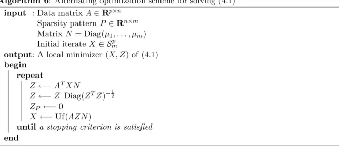
0 0.2 0.4 0.6 0.8 1 0 0.1 0.2 0.3 0.4 0.5 0.6 0.7 0.8 0.9 1
Normalized sparsity inducing parameter
Proportion of nonzero entries
Theoretical upper bound
GPower`1
GPower`0
Figure 2: Dependence of cardinality on the value of the sparsity-inducing parameter γ. In case of the GPower`1 algorithm, the horizontal axis shows γ/kai∗k2, whereas for the
GPower`0 algorithm, we use
√
γ/kai∗k2. The theoretical upper bound is therefor identical for both methods. The plots are averages based on 100 test problems of size p= 100 and n= 300.
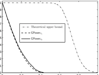
Greedy versus the rest. The considered sparse PCA methods feature different empirical computational complexities. In Figure 3, we display the average time required by the sparse PCA
algorithms to extract one sparse component from Gaussian matrices of dimensionsp= 100 and
n= 300. One immediately notices that the greedy method slows down significantly as cardinality increases, whereas the speed of the other considered algorithms does not depend on cardinality. Since on average Greedy is much slower than the other methods, even for low cardinalities, we discard it from all following numerical experiments.
0 50 100 150 200 250 300 0 1 2 3 4 5 6 7 Cardinality
computational time [sec]
GPower`1 GPower`0 Greedy SPCA rSVD`1 rSVD`0
Figure 3: The computational complexity of Greedy grows significantly if it is set out to output a loading vector of increasing cardinality. The speed of the other methods is unaffected by the cardinality target.
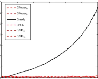
Speed and scaling test. In Tables 3 and 4 we compare the speed of the remaining algorithms. Table 3 deals with problems with a fixed aspect ratio n/p= 10, whereas in Table 4, p is fixed at 500, and exponentially increasing values of n are considered. For the GPower`1
method, the sparsity inducing parameterγ was set to 10% of the upper bound γmax =kai∗k2.
For the GPower`0 method, γ was set to 1% of γmax = kai∗k22 in order to aim for solutions of comparable cardinalities (see (5.2)). These two parameters have also been used for the rSVD`1
and therSVD`0 methods, respectively. ConcerningSPCA, the sparsity parameter has been chosen by trial and error to get, on average, solutions with similar cardinalities as obtained by the other methods. The values displayed in Tables 3 and 4 correspond to the average running times of the algorithms on 100 test instances for each problem size. In both tables, the new methods
GPower`1 andGPower`0 are the fastest. The difference in speed betweenGPower`1 and GPower`0
results from different approaches to fill the active part of z: GPower`1 requires to compute a
rank-one approximation of a submatrix ofA (see Equation (4.2)), whereas the explicit solution (2.11) is available toGPower`0. The linear complexity of the algorithms in the problem sizenis clearly visible in Table 4.
Different convergence mechanisms. Figure 4 illustrates how the trade-off between ex-plained variance and sparsity evolves in the time of computation for the two methodsGPower`1
and rSVD`1. In case of the GPower`1 algorithm, the initialization point (5.1) provides a good approximation of the final cardinality. This method then works on maximizing the variance while keeping the sparsity at a low level throughout. The rSVD` algorithm, in contrast, works
p×n 100×1000 250×2500 500×5000 750×7500 1000×10000 GPower`1 0.10 0.86 2.45 4.28 5.86 GPower`0 0.03 0.42 1.21 2.07 2.85 SPCA 0.24 2.92 14.5 40.7 82.2 rSVD`1 0.21 1.45 6.70 17.9 39.7 rSVD`0 0.20 1.33 6.06 15.7 35.2
Table 3: Average computational time for the extraction of one component (in seconds).
p×n 500×1000 500×2000 500×4000 500×8000 500×16000 GPower`1 0.42 0.92 2.00 4.00 8.54 GPower`0 0.18 0.42 0.96 2.14 4.55 SPCA 5.20 7.20 12.0 22.6 44.7 rSVD`1 1.20 2.53 5.33 11.3 26.7 rSVD`0 1.09 2.26 4.85 10.5 24.6
Table 4: Average computational time for the extraction of one component (in seconds).
in two steps. First, it maximizes the variance, without enforcing sparsity. This corresponds to computing the first principal component and requires thus a first run of the algorithm with random initialization and a sparsity inducing parameter set at zero. In the second run, this parameter is set to a positive value and the method works to rapidly decrease cardinality at the expense of only a modest decrease in explained variance. So, the new algorithmGPower`1 per-forms faster primarily because it combines the two phases into one, simultaneously optimizing the trade-off between variance and sparsity.
0 0.5 1 1.5 2 2.5 3 3.5 0.5 0.6 0.7 0.8 0.9 1
Computational time [sec]
Proportion of explained variance
GPower`1(Variance) rSVD`1(Variance) 0 0.5 1 1.5 2 2.5 3 3.50 0.1 0.2 0.3 0.4 0.5 0.6 0.7 0.8 0.9 1
Computational time [sec]
Proportion of nonzero entries
GPower`1(Cardinality)
rSVD`1(Cardinality)
Figure 4: Evolution of the variance (solid lines and left axis) and cardinality (dashed lines and right axis) in time of computation for the methods GPower`1 and rSVD`1 on a test problem withp= 250 andn= 2500. The vertical axis is the ratio Var(zsPCA)/Var(zPCA), where the loading vectorzsPCA is computed by sparse PCA andzPCA is the first principal loading vector. The rSVD`1 algorithm first solves unconstrained PCA, whereas GPower`1 immediately optimizes the trade-off between variance and sparsity.