On the conditional small ball property of multivariate Lévy-driven moving average processes

(1)

This is a self-archived – parallel published version of this article in the

publication archive of the University of Vaasa. It might differ from the original.

On the conditional small ball property of

multivariate Lévy-driven moving average

processes

Author(s): Pakkanen, Mikko S.; Sottinen, Tommi; Yazigi, Adil

Title: On the conditional small ball property of multivariate Lévy-driven moving average processes

Year: 2017

Version: Accepted manuscript

Please cite the original version:

Pakkanen, M. S., Sottinen, T., & Yazigi, A., (2017). On the conditional small ball property of multivariate Lévy-driven moving average processes. Stochastic Processes and their

Applications 127(3), 749–782.

(2)

MULTIVARIATE L ´EVY-DRIVEN MOVING AVERAGE PROCESSES MIKKO S. PAKKANEN, TOMMI SOTTINEN, AND ADIL YAZIGI

Abstract. We study whether a multivariate Lévy-driven moving average process can shadow arbitrarily closely any continuous path, starting from the present value of the process, with positive conditional probability, which we call the conditional small ball property. Our main results establish the conditional small ball property for Lévy-driven moving average processes under natural non-degeneracy conditions on the kernel function of the process and on the driving Lévy process. We discuss in depth how to verify these conditions in practice. As concrete examples, to which our results apply, we consider fractional Lévy processes and multivariate Lévy-driven Ornstein–Uhlenbeck processes.

1. Introduction

We consider multivariate L´evy-driven moving average processes, i.e.,Rd-valued stochas-tic processesX = (Xt)t>0 defined by the stochastic integral

Xt = Z t

−∞

Φ(t−u)−Ψ(−u)dLu, t>0. (1.1) Here the driving process L = (Lt)t_∈R is a two-sided, d-dimensional L´evy process; and Φ and Ψ are deterministic functions that take values in the space of d×d matrices. Under some integrability conditions, which will be made precise in Section2.2below, the stochastic integral in (1.1) exists in the sense of Rajput and Rosi´nski [37] as a limit in probability.

The process X is infinitely divisible and has stationary increments; in the case Ψ = 0 the process is also stationary. Several interesting processes are special cases of X, including fractional Brownian motion [31], fractional Lévy processes [33], and Lévy-driven Ornstein–Uhlenbeck (OU) processes [6, 42]. Various theoretical aspects of Lévy-driven and Brownian moving average processes, such as semimartingale property, path regularity, stochastic integration, maximal inequalities, and asymptotic behavior of power variations, have attracted a lot of attention recently; see, e.g., [7,8,10,12,13,14,19].

We study in this paper the following theoretical question regarding the infinite-dimen-sional conditional distributions of the processX. Suppose that 06t0< T <∞ and take a continuous path f : [t0, T] → Rd such that f(t0) = Xt0. Can X shadow f within ε

Date: June 25, 2016.

2010Mathematics Subject Classification. Primary 60G10, 60G17; Secondary 60G22, 60G51.

Key words and phrases. Small ball probability, conditional full support, moving average process, mul-tivariate Lévy process, convolution determinant, fractional Lévy process, Lévy-driven OU process, Lévy copula, Lévy mixing, multivariate subordination.

M. S. Pakkanen was partially supported by CREATES (DNRF78), funded by the Danish National Research Foundation, by Aarhus University Research Foundation (project “Stochastic and Econometric Analysis of Commodity Markets”), and by the Academy of Finland (project 258042). T. Sottinen was partially funded by the Finnish Cultural Foundation (National Foundations’ Professor Pool). A. Yazigi was funded by the Finnish Doctoral Programme in Stochastics and Statistics.

(3)

distance on the interval [t0, T] with positive conditional probability, given the history of the process up to timet0, for anyε >0 and any choice off? If the answer is affirmative, we say thatX has theconditional small ball property (CSBP). WhenX is continuous, the CSBP is equivalent to the conditional full support (CFS) property, originally introduced by Guasoni et al. [25], in connection with no-arbitrage and superhedging results for asset pricing models with transaction costs. For recent results on the CFS property, see, e.g., [16,20,23,35,36].

In particular, Cherny [20] has proved the CFS property for univariate Brownian moving average processes. The main results of this paper, stated in Section 2, provide a multi-variate generalization of Cherny’s result and allow for a non-Gaussian multimulti-variate L´evy process as the driving process. Our first main result, Theorem2.7, treats the multivariate Gaussian case (where it leads to no loss of generality if we assume thatX is continuous). Namely, when L is a multivariate Brownian motion, we show that X has CFS provided that the convolution determinant of Φ (see Definition 2.5) does not vanish in a neigh-borhood of zero. The proof of Theorem 2.7 is based on a multivariate generalization of Titchmarsh’s convolution theorem [44], due to Kalisch [26].

Our second main result, Theorem 2.9, covers the case whereL is purely non-Gaussian. Under some regularity conditions, we show that X has the CSBP if the non-degeneracy condition on the convolution determinant of Φ, as seen in the Gaussian case, holds and if

L satisfies a small jumps condition on its Lévy measure: for any ε >0, the origin ofRd is in the interior of the convex hull of the support of the Lévy measure, restricted to the origin-centric ball with radius ε. Roughly speaking, this ensures that the Lévy process

L can move arbitrarily close to any point in Rd with arbitrarily small jumps. We prove Theorem2.9building on a small deviations result for L´evy processes due to Simon [43].

In Section 3, we discuss in detail how to check the assumptions of Theorems2.7and2.9

for concrete processes. First, we provide tools for checking the non-degeneracy condition on the convolution determinant of Φ under various assumption on Φ, including the cases where the components of Φ are regularly varying at zero and where Φ is of exponential form, respectively. As a result, we can show CFS for (univariate) fractional Lévy processes and the CSBP for multivariate Lévy-driven OU processes. Second, we introduce methods of checking the small jumps condition in Theorem2.9, concerning the driving Lévy process

L. We show how to establish the small jumps condition via the polar decomposition of the Lévy measure of L. Moreover, we check the condition for driving Lévy processes whose dependence structure is specified using multivariate subordination [4], Lévy copulas [28], or Lévy mixing [5].

We present the proofs of Theorems 2.7 and 2.9 in Section 4. Additionally, we include Appendices A and B, where we review (and prove) Kalisch’s multivariate extension of Titchmarsh’s convolution theorem and prove two ancillary results on regularly varying functions, respectively. Finally, in AppendixCwe comment on a noteworthy consequence of the CSBP in relation to hitting times.

2. Preliminaries and main results

2.1. Notation and conventions. Throughout the paper, we use the convention that R+ := [0,∞), R++ := (0,∞), and N:= {1,2, . . .}. For any m ∈N and n∈ N, we write Mm,n for the space of real m×n-matrices, using the shorthand Mn forMn,n, andS+n for the cone of symmetric positive semidefinite matrices in Mn. As usual, we identify Mn,1

(4)

with Rn. We denote by h·,·i the Euclidean inner product in Rn. For A ∈ Mm,n, the notationkAk stands for the Frobenius norm ofA, given by Pm

i=1 Pn

j=1A2i,j 1/2

, andA>

for the transpose ofA.

When E is a subset of some topological space X, we write ∂E for the boundary of E, intE for the interior of E, and clE for the closure of E in X. When E ⊂ Rd, we use convE for the convex hull of E, which is the convex set obtained as the intersection of all convex subsets ofRn that contain E as a subset. For any x∈Rn and ε >0, we write

B(x, ε) := {y ∈ _Rn _: _k_x₋_y_k _{< ε}_}_{. Moreover,} _Sn−1 _:= _{_y _∈ _Rn _: _k_y_k _{= 1}_} _{stands for} the unit sphere inRn. For measurable f :R→ Rn, we write ess suppf for the essential support off, which is the smallest closed subset ofRsuch thatf =0 almost everywhere in its complement.

We denote, for anyp >0, byLp_loc(R+,R) the family of real-valued measurable functions

gdefined onR+ such that Z t

0

|g(u)|pdu <∞ for all t>0,

extending them to the real line byg(u) := 0, u <0, when necessary. Moreover, we denote byLp_loc(R+,Mm,n) the family of measurable functionsG:R+→Mm,n, where the (i, j)-th component function u 7→ Gi,j(u) of G belongs to Lp_loc(R+,R) for any i = 1, . . . , m and

j= 1, . . . , n. Similarly, we write G∈Lp(R+,Mm,n) if each of the component functions of

Gbelongs to Lp(R+,R). Note thatL2(R+,Mm,n)⊂L1loc(R+,Mm,n).

Recall that the convolution of g ∈L1_loc(R+,R) and h∈ L1_loc(R+,R), denoted by g∗h, is a function onR+ defined via

(g∗h)(t) := Z t

0

g(t−u)h(u)du, t>0,

and that (g, h)7→g∗his an associative and commutative binary operation onL1_loc(R+,R). We additionally extend the convolution to matrix-valued functions G ∈ L1_loc(R+,Mm,r) andH ∈L1_loc(R+,Mr,n), for anyr ∈N, by defining

(G∗H)i,j(t) := r X

k=1

(Gi,k∗Hk,j)(t), t>0,

for alli= 1, . . . , mand j= 1, . . . , n. It follows from the properties of the convolution of scalar-valued functions thatG∗H∈L1_loc(R+,Mm,n).

When Xis a Polish space (separable topological space with complete metrization), we write B(X) for the Borel σ-algebra of X. When µ is a Borel measure on X, we denote by suppµ the support of µ, which is the set of points x ∈ _X such that µ(A) > 0 for any open A ⊂ X such that x ∈ A. Moreover, if −∞ < u < v < ∞ and x ∈ Rn, then

Cx([u, v],Rn) (resp.Cx1([u, v],Rn)) stands for the family of continuous (resp. continuously

differentiable) functionsf : [u, v]→Rn such thatf(u) =x. We equipCx([u, v],Rn) with the uniform topology induced by the sup norm. Finally, D([u, v],Rn) denotes the space of c`adl`ag (right continuous with left limits) functions f : [u, v]→ _Rn_{, equipped with the} Skorohod topology, andDx([u, v],Rn) its subspace of functionsf ∈D([u, v],Rn) such that

f(u) =x.

2.2. L´evy-driven moving average processes. Fix d ∈ _N and let (Lt)t>0 be a L´evy process inRd, defined on a probability space (Ω,F,P), with characteristic triplet (b,S,Λ),

(5)

where b∈Rd, S∈ S_d+, and Λ is a L´evy measure on Rd, that is, a Borel measure on Rd that satisfies Λ({0}) = 0 and

Z

Rd

min{1,kxk2}Λ(dx)<∞. (2.1) Recall that the processLhas the L´evy–Itˆo representation

Lt:=bt+ Ξ>Wt+ Z t 0 Z {kxk61} xNe(dx,du) + Z t 0 Z {kxk>1} xN(dx,du), t>0,

where Ξ∈Mdis such thatS= Ξ>Ξ,W = (Wt)t>0 is a standard Brownian motion inRd,

N is a Poisson random measure on Rd×[0,∞) with compensator ν(dx,du) := Λ(dx)du and Ne := N −ν is the compensated Poisson random measure corresponding to N. The Brownian motionW and the Poisson random measure N are mutually independent. For a comprehensive treatment of L´evy processes, we refer the reader to the monograph by Sato [41].

Let (L0_t)t>0 be an independent copy of (Lt)t>0. It is well-known that both (Lt)t>0 and (L0_t)t>0admit càdlàg modifications (see, e.g., [27, Theorem 15.1]) and we tacitly work with these modifications. We can then extendL to a càdlàg process onRby

˜

Lt:=Lt1[0,∞)(t) +L0₋t−1(−∞,0)(t), t∈R. (2.2) In what follows we will, for the sake of simplicity, identifyLt with ˜Lt even whent <0.

Let Φ : R → Md and Ψ : R → Md be measurable matrix-valued functions such that Φ(t) = 0 = Ψ(t) for allt <0. Define a kernel function

K(t, u) := Φ(t−u)−Ψ(−u), (t, u)∈R2.

The key object we study in this paper is a causal, stationary-increment moving average processX = (Xt)t>0 driven by L, which is defined by

Xt:= Z t

−∞

K(t, u)dLu, t>0. (2.3) The stochastic integral in (2.3) is defined in the sense of Rajput and Rosi´nski [37] (see also Basse-O’Connor et al. [9]) as a limit in probability, provided that (see [9, Corollary 4.1]) for anyi= 1, . . . , d and t>0,

Z t −∞ hki(t, u),Ski(t, u)idu <∞, (2.4a) Z t −∞ Z Rd min1,hki(t, u),xi2 Λ(dx)du <∞, (2.4b) Z t −∞ hki(t, u),bi+ Z Rd τ1 hki(t, u),xi− hki(t, u), τd(x)iΛ(dx) du <∞, (2.4c) where ki(t, u) ∈ Rd is the i-th row vector of K(t, u), τ1(x) := x1{|x|61}, and τd(x) :=

x1_{kxk61}.

Remark 2.1. When L is a driftless Brownian motion (that is, b = 0 and Λ = 0), the conditions (2.4b) and (2.4c) become vacuous. When det(S) 6= 0, the condition (2.4a) implies thatRt

0 kK(t, u)k2du <∞, which in turn implies that Φ∈L2loc(R+,Md).

In the case where E[kL1k2]<∞, which is equivalent to the condition (2.5) below, we find a more convenient sufficient condition for integrability:

(6)

Lemma 2.2 (Square-integrable case). Suppose that the L´evy measure Λ satisfies

Z

kxk>1

kxk2Λ(dx)<∞. (2.5)

Then conditions (2.4a),(2.4b), and (2.4c) are satisfied provided that

Z t −∞

(kK(t, u)k+kK(t, u)k2)du <∞ for any t>0. (2.6)

Proof. It suffices to only check conditions (2.4b) and (2.4c), condition (2.4a) being evident. Note that (2.5), together with (2.1), implies that R

Rdkxk

2_Λ(d_x₎ _< _∞_{. Thus, by the} Cauchy–Schwarz inequality and (2.6),

Z t −∞ Z Rd min1,hki(t, u),xi2 Λ(dx)du6 Z t −∞ kki(t, u)k2du Z Rd kxk2Λ(dx)<∞,

so (2.4b) is satisfied. To verify (2.4c), we can estimate Z t −∞ hki(t, u),bi+ Z Rd τ1 hki(t, u),xi− hki(t, u), τd(x)iΛ(dx) du 6kbk Z t −∞ kki(t, u)kdu+ Z t −∞ Z {kxk>1} τ₁ hk_i(t, u),xi Λ(dx)du + Z t −∞ Z {kxk61} τ₁ hk_i(t, u),xi − hki(t, u),xiΛ(dx)du, (2.7)

where the first term on the r.h.s. is finite under (2.6). The second term on the r.h.s. of (2.7) can be shown to be finite using Cauchy–Schwarz, viz.,

Z t −∞ Z {kxk>1} τ₁ hk_i(t, u),xi Λ(dx)du6 Z t −∞ kki(t, u)kdu Z {kxk>1} kxkΛ(dx)<∞,

since (2.5) implies that R_{k_x_k>1}kxkΛ(dx) <∞. Finally, to treat the third term on the r.h.s. of (2.7), note that|τ1(x)−x|=|x|1_{|x|>1} 6x2 for any x∈R. Hence,

Z t −∞ Z {kxk61} τ₁ hk_i(t, u),xi − hki(t, u),xi Λ(dx)du 6 Z t −∞ Z {kxk61} hki(t, u),xi2Λ(dx)du 6 Z t −∞ kki(t, u)k2du Z {kxk61} kxk2Λ(dx)<∞, by Cauchy–Schwarz and (2.5).

In the sequel, unless we are considering some specific examples of K, we shall tacitly assume that the integrability conditions (2.4a), (2.4b), and (2.4c) are satisfied.

The following decomposition of X is fundamental; our technical arguments and some of our assumptions rely on it. For anyt0 >0,

Xt=Xt0 + ¯X

t0

(7)

where ¯ Xt0 t := Z t t0 Φ(t−u)dLu, At0 t := Z t0 −∞ Φ(t−u)−Φ(t0−u) dLu. Note that fort0>0 it holds that

Φ(t−u)1_(t₀_,t)(u) =K(t, u)1_(t₀_,t)(u) for any t>t0 and u∈R.

Thus the integrability conditions (2.4a), (2.4b), and (2.4c) ensure that the stochastic integral defining ¯Xt0

t exists in the sense of [37] and, consequently, Att0 is well-defined as well.

2.3. The conditional small ball property. To formulate our main results, we introduce the conditional small ball property (cf. [15, p. 459]):

Definition 2.3. A c`adl`ag process Y = (Yt)t∈[0,T], with values inRd, has theconditional

small ball property (CSBP) with respect to filtration F= (F_t)t∈[0,T], if (i) Y is adapted toF,

(ii) for any t0 ∈[0, T), f ∈C0([t0, T],Rd), andε >0,

P sup t∈[t0,T] kYt−Yt0−f(t)k< ε F_t₀ >0 almost surely. (2.9) If the processY is continuous and satisfies (i) and (ii), then we say thatY hasconditional full support (CFS) with respect to F.

Remark 2.4. (i) The condition (ii) of Definition 2.3 has an equivalent formulation (cf. [15, p. 459]), where the deterministic time t0 ∈ [0, T) in (2.9) is replaced with any stopping timeτ such thatP[τ < T]>0 . The equivalence of this, seemingly stronger, formulation with the original one can be shown adapting the proof of [25, Lemma 2.9].

(ii) More commonly, the CFS property is defined via the condition supp LawP (Yt)t∈[t0,T]

F_t₀

=CY0([t0, T],R

d₎ _{a.s. for any}_t

0∈[0, T), (2.10) where LawP (Yt)t∈[t0,T]

F_t₀

stands for the regular conditional law of (Yt)t∈[t0,T]on C([t0, T],Rd) under P, givenFt0. The equivalence of condition (ii) of Definition2.3

and (2.10) is an obvious extension of [35, Lemma 2.1]. We argue that for discontinuous

Y, the natural generalization of the CFS property would be supp LawP (Yt)t∈[t0,T]

F_t₀

=DY0([t0, T],R

d₎ _{a.s. for any}_t

0∈[0, T), (2.11) where the regular conditional law is now defined on the Skorohod spaceD([t0, T],Rd). The condition (ii) in Definition 2.3 does not imply (2.11), which is why we refer to the property introduced in Definition 2.3 as the CSBP, instead of CFS. The CFS property for discontinuous processes, defined by (2.11), appears to be considerably more difficult to check than the CSBP; and the question whether (discontinuous) L´evy-driven moving average processes have CFS is beyond the scope of the present paper. However, in the context of L´evy processes, the CFS property could be studied using a Skorohod-space support theorem due to Simon [43, Corollaire 1], relying on the independence and stationarity of increments.

(8)

(iii) Suppose thatY has the CSBP (resp. CFS) with respect to F. If ¯Y = Y¯t_t∈[0,T] is a continuous process independent of Y, then the process

Zt:=Yt+ ¯Yt, t∈[0, T],

has the CSBP (resp. CFS) with respect to its natural filtration. This is a straight-forward extension of [23, Lemma 3.2].

(iv) If Y = (Yt)t∈[0,T] has the CSBP with respect to F, then Yt, for any t∈(0, T], has full support inRd, in the sense that

supp LawP(Yt) =Rd.

It is also possible to show thatY is then able to hit any open subset ofRdarbitrarily fast after any stopping time with positive conditional probability. We elaborate on this property in AppendixC.

(v) The CSBP implies the so-called stickiness property, introduced by Guasoni [24], which is a sufficient condition for some no-arbitrage results on market models with frictions. Guasoni [24, Proposition 2.1] showed that any univariate, sticky càdlàg process is arbitrage-free (as a price process) under proportional transaction costs. More recently, Ràsonyi and Sayit [38, Proposition 5.3] have shown that multivariate, sticky càdlàg processes are arbitrage-free under superlinear frictions.

In what follows, we work with the increment filtration FL,inc ₌ _FL,inc t

t∈R, given by

FL_t,inc :=σ(Lu−Lv :−∞< v < u6t).

If we prove that the moving average processX has the CSBP (resp. CFS) with respect to

FL,inc_{, then also the CSBP (resp. CFS) with respect to the (smaller) augmented natural} filtration of X follows, by [35, Lemma 2.2 and Corollary 2.1]. However, we are unable to work with the larger filtration

FL_t :=σ(Lu:−∞< u6t), t∈R,

since the incrementsLu−Lv, t6u < v, are typically not independent of FLt ; see [9] for a discussion. (This independence property is essential in our arguments.)

It is convenient to treat separately the two cases where the L´evy processLis Gaussian (Λ = 0) and purely non-Gaussian (S = 0), respectively. However, we stress that our results make it possible to establish the CSBP/CFS also in the general (mixed) case, where the process X can be expressed as a sum of two mutually independent moving average processes, with a Brownian motion and a purely non-Gaussian L´evy processes as the respective drivers; see Remark2.4(iii).

Let us consider the Gaussian case first. In this case we may assume, without loss of generality, that the moving average process X is continuous — if X were discontinuous, it would have almost surely unbounded trajectories by a result of Belyaev [11].

In his paper [20], Cherny considered the univariate Brownian moving average process

Zt:= Z t

−∞

f(t−s)−f(−s)dBs, t>0,

where f is a measurable function on R+ that satisfies R_−∞t f(t−s)−f(−s)2ds < ∞ for anyt>0 and (Bt)t∈R is a two-sided standard Brownian motion. He showed, see [20, Theorem 1.1], that (Zt)t∈[0,T] has CFS for anyT >0, as long as

(9)

A naive attempt to generalize Cherny’s result to the multivariate moving average pro-cess X in the Gaussian case would be build on the assumption that the components of the kernel function Φ satisfy individually the univariate condition (2.12). However, this would fail to account for the possibility that the components ofX may become perfectly dependent, which would evidently be at variance with the CFS property.

It turns out that a suitable multivariate generalization of the condition (2.12) can be formulated using the following concept:

Definition 2.5. Theconvolution determinant ofG∈L1_loc(R+,Mn) is a real-valued func-tion given by det∗(G)(t) := X σ∈Sn sgn(σ) G1,σ(1)∗ · · · ∗Gn,σ(n) (t), t>0, (2.13) where Sn stands for the group of permutations of the set {1, . . . , n} and sgn(σ) for the signature of σ ∈ Sn. We note that det∗(G) ∈ L1_loc(R+,R) and that the formula (2.13) is in fact identical to the definition of the ordinary determinant, except that products of scalars are replaced with convolutions of functions therein.

Remark 2.6. Unfortunately, the literature on convolution determinants is rather scarce, but convolution determinants are discussed in some books on integral equations; see, e.g., [1]. We review some pertinent properties of the convolution determinant in Appendix A.

In the Gaussian case we obtain the following result, which says that the process X has CFS, provided that the convolution determinant of the kernel function Φ does not vanish near zero. We defer the proof of this result to Section4.1.

Theorem 2.7(Gaussian case). Suppose that the driving L´evy processLis a non-degener-ate Brownian motion, that is,det(S)6= 0 and Λ = 0. Assume, further, that the processes X and At0_{, for any}_t

0 >0, are continuous (modulo taking modifications). If

0∈ess supp det∗(Φ), (DET-∗)

then(Xt)t∈[0,T] has CFS with respect to FLt,inc

t∈[0,T] for anyT >0.

Remark 2.8. (i) One might wonder if it is possible to replace the condition (DET-∗) in Theorem2.7with a slightly weaker condition, analogous to (2.12), namely, that

ess supp det∗(Φ)6=∅. (2.14) Unfortunately, (2.14) does not suffice in general. For example, let Φ(t) = 1[1,2](t)Id and Ψ(t) =1_[0,1](t)Id fort∈R+, whereId∈Md is the identity matrix. Then

det∗(Φ) =1_[1,2]∗ · · · ∗1_[1,2]

| {z }

d

,

which follows immediately from the definition (2.13). One can now show, e.g., using Titchmarsh’s convolution theorem (Lemma A.1, below) and induction in d, that (2.14) holds. However, X1= Z 1 −∞ 1[1,2](1−s)Id−1[0,1](−s)Id dLs= Z 0 −1 dLs− Z 0 −1 dLs =0, which indicates that (Xt)t∈[0,T]cannot have CFS for any T >1.

(10)

(ii) Theorem2.7can be generalized to multivariateBrownian semistationary (BSS) pro-cesses, extending [36, Theorem 3.1], as follows. Let Y = (Yt)t>0 be a continu-ous process in Rd and let Σ = (Σt)t∈R be a measurable process in Md such that sup_t_∈RE[kΣtk2]<∞, both independent of the driving Brownian motionL. Then

Zt:=Yt+ Z t

−∞

Φ(t−s)ΣsdLs, t>0,

defines aBSS process inRd, which has a continuous modification ifQΦ1(h)+QΦ2(h) =

O(hr),h→0+ for somer >0, whereQΦ₁(h) andQΦ₂(h) are quantities related to the

L2 norm and L2 modulus of continuity of Φ, respectively, defined by (3.1) and (3.2) below. In this setting we could show, by adapting the proof of Theorem2.7 and the arguments in [36, pp. 583–585], that if

Leb({t∈[0, T] : det(Σt) = 0}) = 0 a.s.,

then the process (Zt)t∈[0,T] has CFS with respect to its natural filtration for any

T > 0. The assumption that Σ and Y are independent of L could be relaxed somewhat by an obvious multivariate extension of the factor decomposition used in [36, p. 582].

Let us then look into the non-Gaussian case with a pure jump process as the driver

L. In addition to that the condition (DET-∗) continues to hold, it is essential that the gamut of possible jumps ofLis sufficiently rich. Consider for instance the case where the components ofLhave only positive jumps, Ψ = 0, and the elements of Φ are non-negative. It is not difficult to see that the components of the resulting moving average process X

will then be always non-negative — an obvious violation of the CSBP.

To avoid such scenarios, we need to ensure, in particular, that L can move close to any point in Rd with arbitrarily small jumps. To formulate this small jumps condition rigorously, we introduce, for any ε >0, the restriction of the L´evy measure Λ to the ball

B 0, ε) by

Λε(A) := Λ A∩B 0, ε), A∈B(Rd).

We obtain the following result, which we shall prove in Section4.2.

Theorem 2.9 (Non-Gaussian case). Suppose that the driving Lévy process L is purely non-Gaussian, that is, S = 0, and that the components of Φ are of finite variation. Assume, further, thatX is càdlàg andAt0_{, for any} _t

0>0, is continuous (modulo taking

modifications). IfΦ satisfies (DET-∗), and if

0∈int conv supp Λε for anyε >0, (JUMPS)

then(Xt)t∈[0,T] has the CSBP with respect to FLt,inc

t∈[0,T] for anyT >0.

Remark 2.10. (i) The proof of Theorem2.9 hinges on the assumption that the compo-nents of Φ are of finite variation. However, we believe that it should be possible to weaken this assumption to boundedness. Rosi´nski [39] has shown that the fine prop-erties of the sample paths of X are inherited from the fine properties of Φ. As the fine properties ofX are not actually “seen” by the sup norm used in the definition of the CSBP, it seems plausible that the finite variation assumption is immaterial and merely a limitation of the machinery used in the present proof.

(11)

(ii) In the univariate case, d= 1, the condition (JUMPS) reduces to the simple require-ment (cf. [2, Proposition 1.1]) that

Λ (−ε,0)>0 and Λ (0, ε)>0 for any ε >0, (JUMPS1) which evidently rules out all processes with only positive jumps (e.g., Poisson pro-cesses) as drivers.

(iii) The condition (JUMPS) could be replaced with a weaker, but more technical, con-dition that would require a similar support property to hold merely in the subspace

HΛ:= y∈_Rd: Z {kxk61} |hx,yi|Λ(dx)<∞ ,

where the jump activity of L has finite variation. In particular, if L has infinite variation in all directions in Rd in the sense that HΛ ={0}, then (JUMPS) can be dropped altogether. (In fact,HΛ={0}can be shown to imply (JUMPS).)

3. Applications and examples

In this section, we discuss how to verify the conditions (DET-∗) and (JUMPS) that appear in Theorems2.7and2.9, and provide some concrete examples of processes, to which these results can be applied. However, first we look into the path regularity conditions of Theorems2.7 and2.9.

3.1. Regularity conditions. We have assumed in Theorems2.7and2.9that the process

At0 _{is continuous for any}_t

0 >0 and thatX is continuous (resp. c`adl`ag) in Theorem 2.7 (resp. Theorem 2.9). Unfortunately, there are no easily applicable, fully general results that could be used to check these conditions, and they need to be established more-or-less on a case-by-case basis.

In the case where E[kL1k2]<∞ and E[L1] = 0, fairly tractable sufficient criteria for these regularity conditions can be given. To this end, define

QΦ₁(h) := Z h 0 kΦ(u)k2du, (3.1) QΦ₂(h) := Z ∞ 0 kΦ(u+h)−Φ(u)k2du. (3.2) Using [33, Proposition 2.1], we find that for any t0 >0,

E[kXt+h−Xtk2]6E[kL1k2] QΦ1(h) +QΦ2(h) , t>0, h>0, (3.3) EAt0 t+h−A t0 t 2 6E[kL1k2]QΦ2(h), t>t0, h>0. (3.4) Thus,At0 _{has a continuous modification by the Kolmogorov–Chentsov criterion if}_QΦ

2(h) =

O(hr2_), _h _→ _{0+, for some} _r

2 > 1. If additionally QΦ1(h) = O(hr1), h → 0+, for some

r1 > 1, then X has a continuous modification as well. (When L is Gaussian, ri > 0,

i= 1,2, suffices.)

WhenAt0 _{is known, a priori, to be continuous for any}_t

0>0, it follows from (2.8), with

t0 = 0, that the processX is continuous (resp. c`adl`ag) provided that ¯

X0_t = Z t

0

Φ(t−u)dLu, t>0,

is continuous (resp. c`adl`ag). The path regularity of ¯X0 becomes an intricate question whenLis purely non-Gaussian. Then, a necessary condition for ¯X0 to have almost surely

(12)

bounded trajectories — which is also necessary for the c`adl`ag property — is that Φ is bounded [39, Theorem 4]. For ¯X0 to be continuous, it is necessary that Φ is continuous and that Φ(0) = 0 [39, Theorem 4]. While necessary, these two conditions are not sufficient for the continuity of ¯X0, however; see [29, Theorem 3.1].

Basse and Pedersen [8] have obtained sufficient conditions for the continuity of the process ¯X0. In particular, their results ensure that, in the case where the components of

Lare of finite variation (S= 0 andHΛ =Rd; see Remark2.10(iii)), ¯X0 is càdlàg (and of finite variation) if the elements of Φ are of finite variation (which is one of the assumptions used in Theorem 2.9). In the case where L is of infinite variation, the corresponding sufficient condition is more subtle; we refer to [8, Theorem 3.1] for details. Finally, we mention the results of Marcus and Rosiński [32] concerning the continuity of infinitely divisible processes using majorizing measures and metric entropy conditions, which could be applied to study the continuity ofX, ¯Xt0

, and At0_,_t

0 >0. 3.2. Kernel functions that satisfy (DET-∗).

3.2.1. The Mandelbrot–Van Ness kernel function. Consider the univariate case, d = 1, where the processes X and L reduce to univariate processes X and L and the kernel functions Φ and Ψ to real-valued functionsφandψ, respectively. Define, for anyH∈(0,1),

φ(t) :=ψ(t) :=CHt H−1

2

+ , t∈R, (3.5)

wherex+:= max{x,0}for any x∈Rand

CH := p

2Hsin(πH)Γ(2H) Γ(H+1₂) ,

which is defined using thegamma function Γ(t) :=R₀∞xt−1e−xdx,t >0. Then

k(t, s) :=φ(t−s)−ψ(−s) =CH (t−s)H− 1 2 + −(−s) H−1 2 + , (t, s)∈_R2,

is the so-called Mandelbrot–Van Ness kernel function (introduced in [31]) of fractional Brownian motion (fBm). That is, with a standard Brownian motion as the driverL, the univariate moving average process

Xt= Z t

−∞

k(t, s)dLs, t>0, (3.6) is an fBm with Hurst indexH∈(0,1).

Eschewing the fBm, which is already known to have CFS (see [20]), we consider the process (3.6) in the case where the driver L is purely non-Gaussian. Such a processX is called afractional L´evy process, introduced by Marquardt [33]. It was shown in [33], that ifH ∈(1₂,1), E[L2₁]<∞ and E[L1] = 0, then the fractional L´evy process is well-defined (conditions (2.4a), (2.4b), and (2.4c) are satisfied) and has a continuous modification. As a consequence of Theorem2.9, we obtain:

Corollary 3.1(Fractional L´evy process). Let(Xt)t∈R+ be a fractional L´evy process, given

by (3.6), with H ∈ (1₂,1) and a purely non-Gaussian driving L´evy process L such that E[L2₁]<∞andE[L1] = 0. If the L´evy measureΛofLsatisfies(JUMPS1), then(Xt)t∈[0,T]

has CFS with respect to FL,inc_t

(13)

Proof. The kernel function φ, given by (3.5), is monotonic and, thus, of finite variation. Additionally, it clearly satisfies the univariate version of the condition (DET-∗), namely,

0∈ess suppφ. (3.7)

The path regularity conditions of Theorem2.9 can be checked via the criteria (3.3) and

(3.4) using [33, Theorem 4.1].

3.2.2. Regularly varying kernel functions. The Mandelbrot–Van Ness kernel function can be generalized by retaining the power-law behavior ofφnear zero, but allowing for more general behavior near infinity. This makes it possible to define processes that, say, behave locally like the fBm, in terms of H¨older regularity, but are not long-range dependent. (In effect, this amounts to dispensing with the self-similarity property of the fBm.)

A convenient way to construct such generalizations is to use the concept of regular variation (see [17] for a treatise on the theory of regular variation). Let us recall the basic definitions:

Definition 3.2. (i) A measurable function h:R+ →R+ is slowly varying at zero if lim

t→0+

h(`t)

h(t) = 1, for all ` >0.

(ii) A measurable function f :R+→ R+ is regularly varying at zero, with index α∈R, if lim t→0+ f(`t) f(t) =` α_, _{for all} _{` >}_0. We write thenf ∈R₀(α).

Remark 3.3. Clearly,f ∈R0(α) if and only iff(t) =tαh(t),t >0, for some slowly varying functionh. Intuitively,f behaves then near zero essentially like the power functiont7→tα, as the slowly varying functionh varies “less” than any power function near zero, in view ofPotter’s bounds (Lemma B.1 in AppendixB).

We discuss now, how to check the condition (DET-∗) for a multivariate kernel function Φ, whose components are regularly varying at zero. Checking (DET-∗) is then greatly facilitated by the fact that convolution and addition preserve the regular variation property at zero. We prove the first of the following two lemmas in AppendixB, while the second follows from an analogous result for regular variation at infinity [17, Proposition 1.5.7(iii)], sincef ∈R0(α) if and only if x7→ f(1/x) is regularly varying at infinity with index −α; see [17, pp. 17–18].

Lemma 3.4 (Convolution and regular variation at zero). Suppose that f ∈ R0(α)∩

L1_loc(R+,R+) and g∈R0(β)∩L1loc(R+,R+) for some α >−1 and β >−1. Then,

(f∗g)(t)∼B(α+ 1, β+ 1)tf(t)g(t), t→0+, (3.8)

where B(t, u) := R₀1su−1(1−s)t−1ds, (t, u) ∈ _R2₊₊, is the beta function. Consequently,

f∗g∈R0(α+β+ 1).

Lemma 3.5 (Addition and regular variation at zero). If f ∈ R₀(α) and g ∈ R₀(β) for someα∈_R andβ ∈_R, then f+g∈R0(min{α, β}).

Using Lemmas3.4and3.5, we can establish (DET-∗) for regularly varying multivariate kernel functions under an algebraic constraint on the indices of regular variation.

(14)

Proposition 3.6 (Regularly varying kernels). Let d>2 and let Φ = [Φi,j]_{(i,j)∈{1,...,d}}2 ∈ L1_loc(R+,Md) be such that Φi,j ∈R0(αi,j) for some αi,j > −1 for all (i, j) ∈ {1, . . . , d}2.

Define

α± := min{α_1,σ(1)+· · ·+α_d,σ(d):σ∈Sd,sgn(σ) =±1}.

If α+6=α−, then Φ satisfies (DET-∗).

Remark 3.7. (i) In the bivariate case,d= 2, the conditionα+6=α− simplifies to

α1,1+α2,2 6=α1,2+α2,1. (3.9) (ii) The condition α+ 6=α− is far from optimal, as it relies on fairly crude information (the indices of regular variation) on the components of Φ. To illustrate this, consider for example Φ(t) := tα1,1 _tα1,2 tα2,1 _tα2,2 , t >0, whereα1,1, α1,2, α2,1, α2,2 >−1. We have det∗(Φ)(t) = B(α1,1+ 1, α2,2+ 1)tα1,1+α2,2+1 −B(α2,1+ 1, α1,2+ 1)tα2,1+α1,2+1, t>0.

Take, say,α1,1 = 2, α1,2 = 1, α2,1 = 3, and α2,2 = 2. Then (3.9) does not hold but (DET-∗) holds since B(3,3)6= B(2,4).

(iii) The definition of regular variation dictates that, under the assumptions of Proposition

3.6, the elements of Φ must be non-negative, which may be too restrictive. To remove this constraint, it is useful to note that if Φ satisfies (DET-∗) then the kernelAΦ(t),

t∈R+, for any invertibleA∈Md also satisfies (DET-∗); see LemmaA.3(i).

Proof of Proposition 3.6. Write first det∗(Φ) = X σ∈Sd:sgn(σ)=1 Φ_1,σ(1)∗ · · · ∗Φ_d,σ(d) | {z } =:φ+ − X σ∈Sd:sgn(σ)=−1 Φ_1,σ(1)∗ · · · ∗Φ_d,σ(d), | {z } =:φ−

and note that, by Lemmas 3.4 and 3.5, we have φ± ∈ R₀(α±+d−1). As a difference of two functions that are regularly varying at zero with different indices, the convolution determinant det∗(Φ) cannot vanish in a neighborhood of zero, in view of Potter’s bounds (LemmaB.1, below). Thus, Φ satisfies (DET-∗). 3.2.3. Triangular kernel functions. When the kernel function Φ isupper orlower triangu-lar, the condition (DET-∗) becomes very straightforward to check. In fact, it suffices that the diagonal elements of Φ satisfy the univariate counterpart of (DET-∗).

Proposition 3.8(Triangular kernel functions). Let d>2 and letΦ = [Φi,j](i,j)∈{1,...,d}2 ∈ L1_loc(R+,Md) be such that i < j ⇒Φi,j= 0 or i > j ⇒Φi,j = 0. If

0∈ess supp Φi,i for any i= 1, . . . , d, (3.10)

thenΦ satisfies (DET-∗).

Proof. When Φ is upper or lower triangular, we find that det∗(Φ) = Φ1,1∗ · · · ∗Φd,d,

(15)

since, in the definition (2.13), any summand corresponding to a non-identity permutation

σ equals zero, as such a summand involves components of Φ above and below the diago-nal. The condition (DET-∗) can then be shown to follow from (3.10) using Titchmarsh’s convolution theorem (LemmaA.1, below) and induction ind. 3.2.4. Exponential kernel functions. In the univariate case, d= 1 (adopting the notation of Section3.2.1), by setting ψ= 0 and

φ(t) :=eat, t>0, (3.11) for some a < 0, the moving average process X becomes an Ornstein–Uhlenbeck (OU) process. It is then clear thatφ satisfies the univariate counterpart (3.7) of the condition (DET-∗).

Multivariate OU processes are defined using the matrix exponential

eA:= ∞ X j=0 1 j!A j_,

where A0 := Id. (The matrix exponential eA ∈ Md is well-defined for any A ∈ Md.) More precisely, we define a matrix-valued kernel function Φ by replacing the parameter

a <0 in (3.11) with a matrix A∈_Md whose eigenvalues have strictly negative real parts. Recall that such matrices are calledstable. We find that such a kernel function Φ satisfies (DET-∗) as well:

Proposition 3.9 (Exponential kernels). Suppose that

Φ(t) =eAt, t>0, (3.12)

for some stableA∈_Md. Then Φ∈Lp(R+,Md) for any p >0, and Φsatisfies (DET-∗).

Proof. The assumption that A is stable implies (see [45, pp. 972–973]) that there exist constantsc=c(A)>0 andβ =β(A)>0 such that

kΦ(t)k=keAtk₆ce−βt for all t>0, which clearly implies that Φ∈Lp(R+,Md) for anyp >0.

To show that Φ satisfies (DET-∗), we consider the Laplace transformL[det∗(Φ)]. Note first that since Φ∈L1(R+,Md), each of the components of Φ belongs toL1(R+,R), whence det∗(Φ) ∈ L1(R+,R). Thus, L[det∗(Φ)](s) exists for any s > 0. By the convolution theorem for the Laplace transform, we have

L[det∗(Φ)](s) = det L[Φ](s)

, s>0. (3.13) We can now use the well-known fact that the Laplace transform of a matrix-valued function of the form (3.12) can be expressed using the resolvent ofA, namely,

L[Φ](s) = (sId−A)−1, s>0. (3.14) Applying (3.14) to (3.13), we get det L[Φ](s) = 1 sddet(Id−s−1A) , s >0, whence L[det∗(Φ)](s)∼ 1 sd, s→ ∞. (3.15)

(16)

Suppose now that Φ does not satisfy (DET-∗), which entails that there is ε > 0 such that det∗(Φ)(t) = 0 for almost every t∈[0, ε]. Thus, for anys>0,

As det∗(Φ) ∈ L1(R+,R), we find that its Laplace transform decays exponentially fast,

which contradicts (3.15).

Corollary 3.10 (L´evy-driven OU process). Suppose that L satisfies E[kL1k2]<∞ and

E[L1] =0. LetX be a stationary L´evy-driven OU process given by

Xt:= Z t

−∞

eA(t−s)ΣdLs, t>0,

for some stableA∈Md and Σ∈Md such that det(Σ)6= 0.

(i) If S = 0 and Λ satisfies (JUMPS), then (Xt)t∈[0,T] has the CSBP with respect to

F_tL,inc

t∈[0,T] for any T >0.

(ii) If Λ = 0 and det(S)6= 0, then (Xt)t∈[0,T] has CFS with respect to FtL,inc

t∈[0,T] for

any T >0

Proof. (i) The kernel function Φ(t) := eAtΣ, t > 0, is clearly of finite variation and, by Proposition 3.9 and Lemma A.3(i), it satisfies (DET-∗). For any t0 > 0, we have the decomposition Xt−Xt0 = (eA(t−t 0)₋_I d)Xt0 | {z } =At0 t +eAt Z t t0 e−AsΣdLs | {z } = ¯Xt0 t , t>t0. (3.16)

Since the mapt7→eAt is continuous,At0 _{is a continuous process. Moreover, as a product}

of a continuous function and a c`adl`ag martingale, ¯Xt0

is càdlàg, soX is càdlàg as well. The assertion follows then from Theorem2.9.

(ii) Theorem 2.7 can be applied here; the continuity of X and At0 _{for any} _t

0 >0 can

deduced from the decomposition (3.16).

3.3. L´evy measures that satisfy (JUMPS).

3.3.1. Polar decomposition. When d>2, the L´evy measure Λ has a polar decomposition (see [40, Proposition 4.1] and [3, Lemma 2.1]),

Λ(A) = Z Sd−1 Z R++ 1A(ru)ρu(dr)ζ(du), A∈B(Rd), (3.17) whereζ is a finite measure on the unit sphereSd−1 ⊂_Rd_and_{_ρ

u:u∈Sd−1}is a family of

L´evy measures onR++such that the mapu7→ρu(A) is measurable for anyA∈B(R++).

Referring to (3.17), we say that Λ admits a polar decomposition{ζ, ρu :u∈Sd−1}.

The condition (JUMPS) can be established via a polar decomposition as follows:

Proposition 3.11(Polar decomposition). Suppose thatd>2 and that the L´evy measure

(17)

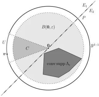
v U P E1 E2 C Sd−1 conv supp Λε B(0, ε) 0

Figure 1. The sets defined in the proof of Proposition3.11.

(i) 0∈int conv suppζ, (ii) ρu (0, ε)

>0 for ζ-almost anyu∈Sd−1 and for any ε >0, thenΛ satisfies (JUMPS).

Proof. Suppose that Λ does not satisfy (JUMPS). Then there existsε >0 such that either

0 ∈∂conv supp Λε or0 ∈/ conv supp Λε. Invoking the supporting hyperplane theorem in the former case and the separating hyperplane theorem in the latter case, we can find a hyperplaneP, passing through 0, that divides Rd into two closed half-spaces E1 and E2 such that E1 ∩E2 = P and that supp Λε ⊂ E2, say. (See Figure 1 for an illustration.) By property (i), we can findv ∈suppζ such that v ∈ intE1. Moreover, we can find an open neighbourhoodU ⊂Sd−1 ofvsuch that U ⊂intE1 andζ(U)>0. Consider now the truncated cone

C :={ru:r ∈(0, ε),u∈U} ⊂B(0, ε),

Clearly, 1C(ru) = 1(0,ε)(r)1U(u) for any r > 0 and u ∈ Sd−1. Thus, by the polar decomposition, we have that

Λε(C) = Λ(C) = Z Sd−1 Z (0,∞) 1_(0,ε)(r)1U(u)ρu(dr)ζ(du) = Z U ρu (0, ε) ζ(du)>0,

where the final inequality follows from property (ii). As the setC has positive Λε-measure, it must intersect supp Λε, which is a contradiction since C ⊂ intE1 and supp Λε ⊂ E2,

whileE2∩ intE1=∅.

Example 3.12. Suppose thatL is a pure jump L´evy process with mutually independent, non-degenerate components (Li_t)t∈R, i = 1, . . . , d. Then the L´evy measure Λ of L is concentrated on the coordinate axes of Rd; see, e.g., [41, Exercise 12.10, p. 67]. More

(18)

concretely, Λ admits then a polar decomposition{ζ, ρu:u∈Sd−1}, with ζ = d X i=1 (δei+δ−ei),

whereδx denotes the Dirac measure atx∈Rdand ei is thei-th canonical basis vector of Rd, and for anyi= 1, . . . , dand A∈B(R++),

ρei(A) =λi(A) and ρ−ei(A) =λi(−A),

whereλi denotes the the L´evy measure of the component (Lit)t∈R.

Clearly, ζ satisfies the condition (i) of Proposition 3.11 and (ii) holds provided that the L´evy measure λi, for any i = 1, . . . , d, satisfies the condition (JUMPS1), namely,

λi (−ε,0)

>0 andλi (0, ε)

>0 for any ε >0.

Example 3.13. It is well known that the L´evy process L is self-decomposable (see [41, Section 3.15] for the usual definition) if and only if its L´evy measure Λ admits a polar decomposition{ζ, ρu:u∈Sd−1}, where

ρu(dr) =

K(u, r)

r dr, ζ-almost every u∈S

d−1_,

for some functionK:Sd−1×_R++→_R+such thatK(u, r) is measurable inuand decreas-ing inr [41, Theorem 15.10, p. 95]. For example, forα∈(0,2), settingK(u, r) :=r−α for all u∈ Sd−1 and r >0, we recover the subclass of α-stable processes [41, Theorem 14.3, pp. 77–78]. Clearly, the condition (ii) in Proposition3.11is then met if sup_r>0K(u, r)>0 forζ-almost everyu∈Sd−1.

3.3.2. Multivariate subordination. Subordination is a classical method of constructing a new Lévy process by time-changing an existing Lévy process with an independent sub-ordinator, a Lévy process with non-decreasing trajectories; see, e.g., [41, Chapter 6]. Barndorff-Nielsen et al. [4] have introduced a multivariate extension of this technique, which, in particular, provides a way of constructing multivariate Lévy processes with dependent components (starting from Lévy processes whose components are mutually independent).

We discuss now, how the condition (JUMPS) can be checked when Λ is the Lévy mea-sure of a Lévy process L that has been constructed by multivariate subordination. For simplicity, we consider only a special case of the rather general framework introduced in [4]. As the key ingredient in multivariate subordination we take a family of d>2 mutu-ally independent, univariate Lévy processes Lei_t

t>0,i= 1, . . . , d, with respective triplets ˜_b_i_,₀_,_λ˜_i

, i = 1, . . . , d. (We eschew Gaussian parts here, as they would be irrelevant in the context of Theorem2.9.) Additionally, we need ad-dimensional subordinator (Tt)t>0, independent of Lei_t

t>0,i= 1, . . . , d, which is a L´evy process whose triplet (c,0, ρ) satisfies

c= (c1, . . . , cd)∈ Rd+ and suppρ⊂ Rd+. We denote the components ofTt by Tt1, . . . , Ttd for any t>0.

By [4, Theorem 3.3], the time-changed process

Lt:= e L1_T1 t, . . . , e Ld_Td t , t>0, (3.18)

(19)

is a L´evy process with triplet (b,0,Λ) given by b:= Z Rd+ ρ(ds) Z {kxk61} xµs(dx) + (c1˜b1, . . . , cd˜bd), Λ(B) := Z Rd+ µs(B)ρ(ds) + Z B c11A1(x)˜λ1(dx1) +· · ·+cd1Ad(x)˜λd(dxd) , B ∈B(Rd), (3.19) where µs(dx) :=P h e L1_s₁ ∈dx1, . . . ,Led_s d∈dxd i = d Y j=1 P h e Lj_s_j ∈dxj i , s∈_Rd₊,

andA_i:={x∈_Rd:xj = 0, j6=i}is the i-th coordinate axis for anyi= 1, . . . , d. (While (3.18) defines only a one-sided processL, it can obviously be extended to a two-sided L´evy process using the construction (2.2).)

Proposition 3.14 (Multivariate subordination). Suppose that the L´evy measure Λ is given by (3.19) and that

˜

λi (−ε,0)

>0 and λ˜i (0, ε)

>0 for any i= 1, . . . , d and ε >0. (3.20)

If c∈_Rd

++ or Rd++∩suppρ=∅, then Λ satisfies (JUMPS).

Proof. Leti= (i1, . . . , id)∈ {0,1}d,ε >0, andB =B1× · · · ×Bd⊂B(0, ε), where

Bj :=    0,√ε d , ij = 1, −√ε d,0 , ij = 0, for any j= 1, . . . , d. We observe that

Λε(B) = Λ(B)> Z B c11A1(x)˜λ1(dx1)+· · ·+cd1Ad(x)˜λd(dxd) = d X i=1 ciλ˜(Bi)>0, (3.21) whenc∈_Rd

++. The assumption (3.20) implies, by Lemma 4.5below, that suppµs=Rd, and consequentlyµs(B)>0, for any s∈Rd++. Thus,

Λε(B) = Λ(B)> Z

Rd++

µs(B)ρ(ds)>0, (3.22)

when Rd++∩suppρ = ∅. It follows from (3.21) and (3.22), that supp Λε intersects with any open orthant ofRd, which in turn implies that Λ satisfies (JUMPS). 3.3.3. Lévy copulas. Letd>2. The Lévy measure Λ onRdcan be defined by specifyingd one-dimensional marginal Lévy measures and describing the dependence structure through aLévy copula, a concept introduced by Kallsen and Tankov [28]. We provide first a very brief introduction to Lévy copulas, following [28].

Below, R:= (−∞,∞]. Moreover, for a= (a1, . . . , ad),b= (b1, . . . , bd)∈ Rd, we write

a6b(resp.a<b) ifai6bi (resp.ai< bi) for anyi= 1, . . . , d. For anya6bwe denote by (a,b] the hyperrectangle Qd_i=1(ai, bi].

(20)

Definition 3.15. LetF :Rd→Rdand leta,b∈Rdbe such thata6b. Therectangular

increment of F over the hyperrectangle (a,b]⊂Rd is defined by

F (a,b]:= X i∈{0,1}d (−1)d− Pd j=1ij_F ₍₁₋_i 1)a1+i1b1, . . . ,(1−id)ad+idbd .

We say thatF isd-increasing ifF (a,b]

>0 for anya,b∈Rdsuch thata6b. Further, we say thatF isstrictly d-increasing ifF (a,b]>0 for any a,b∈_Rdsuch that a<b.

Definition 3.16. Let F : Rd → Rd be d-increasing, with F(x1, . . . , xd) = 0 whenever

xi = 0 for some i= 1, . . . , d. For any non-empty I ⊂ {1, . . . , d}, theI-margin of F is a functionFI :R|I|→Rgiven by FI (xi)i∈I:= lim_u →−∞ X (xi)i∈Ic∈{u,∞}|Ic| F(x1, . . . , xd) Y i∈Ic sgn(xi),

where sgn(x) := −1_(−∞,0)(x) +1_[0,∞)(x), x ∈ _R, and Ic stands for the complement

{1, . . . , d} \I.

Definition 3.17. Ad-dimensionalL´evy copula is a functionC :Rd→Rsuch that (i) C(x1. . . , xd)<∞ whenxi<∞for all i= 1. . . , d,

(ii) C(x1. . . , xd) = 0 whenxi= 0 for some i= 1. . . , d, (iii) C isd-increasing,

(iv) C{i}(x) =x for all x∈_Rand i= 1. . . , d.

Remark 3.18. The properties (ii), (iii), and (iv) of a L´evy copula are analogous to the defining properties of a classical copula; see, e.g., [34, Definition 2.10.6].

Recall that a classical copula describes a probability measure on Rd through its cumu-lative distribution function, by Sklar’s theorem [34, Theorem 2.10.9]. In the context of L´evy copulas, the cumulative distribution function is replaced with the tail integral of the L´evy measure, which is defined as follows.

Definition 3.19. Thetail integral of the L´evy measure Λ is a functionJΛ: (R\{0})d→R given by JΛ(x1, . . . , xd) := Λ d Y j=1 I(xj) d Y i=1 sgn(xi), where I(x) := ( (x,∞), x>0, (−∞, x], x <0.

Definition 3.20. Let I ⊂ {1, . . . , d} be non-empty. The I-marginal tail integral of the L´evy measure Λ, denoted byJ_ΛI, is the tail integral of the L´evy measure ΛI of the process

LI := (Li)_i∈I, which consists of components of the Lévy process L with Lévy measure Λ. Kallsen and Tankov [28, Lemma 3.5] have shown that the Lévy measure Λ is fully determined by its marginal tail integralsJ_ΛI,I ⊂ {1, . . . , d} is non-empty. Moreover, they have proved a Sklar’s theorem for Lévy copulas [28, Theorem 3.6], which says that for any Lévy measure Λ onRd, there exists a Lévy copula C that satisfies

J_ΛI (xi)i∈I=CI J_Λ{i}(xi) i∈I

(21)

for any non-empty I ⊂ {1, . . . , d} and any (xi)_i∈I ∈ (R\ {0})|I|. Conversely, we can construct Λ from a L´evy copula C and (one-dimensional) marginal L´evy measures λi,

i= 1, . . . , d, by defining J_ΛI (xi)i∈I :=CI Jλi(xi) i∈I

for any non-emptyI ⊂ {1, . . . , d} and any (xi)i∈I ∈(R\ {0})|I|. Then we say that Λ has L´evy copula C and marginal L´evy measuresλi,i= 1, . . . , d.

We can now show that Λ satisfies (JUMPS) if it has strictlyd-increasing L´evy copula and marginal L´evy measures such that each of them satisfies (JUMPS1).

Proposition 3.21 (Lévy copula). Suppose that the Lévy measure Λ has Lévy copula C

and marginal L´evy measuresλi, i= 1, . . . , d. If

(i) C is strictly d-increasing, (ii) λi (−ε,0)

>0 and λi (0, ε)

>0 for any i= 1, . . . , dand ε >0, thenΛ satisfies (JUMPS).

Remark 3.22. Proposition3.21has the caveat that its assumptions do not cover the case where Λ is the Lévy measure of a Lévy process with independent components, discussed in Example 3.12. Indeed, the corresponding “independence Lévy copula”, characterized in [28, Proposition 4.1], is not strictlyd-increasing. However, it is worth pointing out that it is not sufficient in Proposition3.21 that C is merely d-increasing, as this requirement is met by all Lévy copulas, including those that give rise to Lévy processes with perfectly dependent components; see, e.g., [28, Theorem 4.4].

Proof of Proposition 3.21. Let a,b ∈ _Rd be such that a 6 b and aibi > 0 for any i = 1, . . . , d. Then JΛ((a,b]) = X i∈{0,1}d (−1)d− Pd j=1ij_J Λ (1−i1)a1+i1b1, . . . ,(1−id)ad+idbd , (3.23) where JΛ (1−i1)a1+i1b1, . . . ,(1−id)ad+idbd =C Jλ1 (1−i1)a1+i1b1 , . . . , Jλd (1−id)ad+idbd =C i1Jλ1(b1) + (1−i1)Jλ1(a1), . . . , idJλd(bd) + (1−id)Jλd(ad) . (3.24)

It follows from Definition3.19 thatx7→Jλi(x) is non-increasing on the intervals (−∞,0)

and (0,∞) for anyi= 1, . . . , d. Thus, ˜ b:= Jλ1(b1), . . . , Jλd(bd) 6 Jλ1(a1), . . . , Jλd(ad) =: ˜a. (3.25) Furthermore, by (3.23) and (3.24), (−1)dJν((a,b]) =C (˜b,a˜] .

We establish (JUMPS) by showing that the intersection of each open orthant ofRdwith supp Λε is non-empty for anyε >0. To this end, letε >0,n∈N, andi∈ {0,1}d. Define

a,b∈_Rd by a:= √ ε d+ 1 i1 n −(1−i1), . . . , id n −(1−id) , b:= √ ε d+ 1 i1− 1−i1 n , . . . , id− 1−id n .

(22)

Note thata6band that (a,b]⊂B(0, ε). Moreover, (a,b] belongs to the open orthant

{(x1, . . . , xd)∈Rd: (−1)1−ijxj >0, j= 1, . . . , d},

It suffices now to show that Λ((a,b]) > 0 for some n ∈ _N. Since aibi > 0 for any

i= 1, . . . , d, we have (cf. the proof of [28, Lemma 3.5])

Λ((a,b]) = (−1)dJΛ((a,b]) =C (˜b,a˜],

where ˜a and ˜bare derived from a andbvia (3.25). Observe that for anyj= 1, . . . , d,

˜ aj−˜bj =Jλj(aj)−Jλj(bj) =    λj _n√ε_d+1,√_d+1ε , ij = 1, λj √−_d+1ε ,_n√−_d+1ε , ij = 0.

It follows now from the assumption (ii) that for some sufficiently large n ≥ 2, we have ˜_b_j _<_˜_a_j _{for any} _j _{= 1}_{, . . . , d}_{, that is, ˜}_b_< _a_˜_{. Thanks to the assumption (}_i_{), we can then} conclude that Λ((a,b]) =C (˜b,a˜]>0.

Example 3.23. We provide here a simple example of ad-strictly increasing L´evy copula, following the construction — which parallels that of Archimedean copulas [34, Chapter 4] in the classical setting — given by Kallsen and Tankov [28, Theorem 6.1]. Suppose that

ϕ: [−1,1]→[−∞,∞] is some strictly increasing continuous function such thatϕ(1) =∞,

ϕ(0) = 0, andϕ(−1) =−∞. Assume, moreover, thatϕisdtimes differentiable on (−1,0) and (0,1), so that

ddϕ(ex)

dxd >0 and

ddϕ(−ex)

dxd <0 for any x∈(−∞,0). (3.26) In [28, Theorem 6.1] it has been shown that the function

C(x1, . . . , xd) :=ϕ d Y i=1 ˜ ϕ−1(xi) ! , (x1, . . . , xd)∈Rd,

where ˜ϕ(x) := 2d−2 ϕ(x)−ϕ(−x), x ∈ [−1,1], is a L´evy copula. (In fact, in [28] the L´evy copula property is shown under weaker assumptions with non-strict inequalities in (3.26).) The argument used in the proof of [28, Theorem 6.1] to show thatCisd-increasing translates easily to a proof thatC is also strictlyd-increasing under (3.26). One can take, e.g.,ϕ(x) := ₁_−|x_x_|,x∈[−1,1], which satisfies the conditions above. In particular,

ddϕ(x) dxd = d! (1−x)d+1 >0, x∈(0,1), (−1)dd d_ϕ₍_x₎ dxd =− d! (1 +x)d+1 <0, x∈(−1,0), which ensure that (3.26) holds.

3.3.4. Lévy mixing. It is also possible to define new Lévy measures onRd, for d>2, by mixing suitable transformations of a given Lévy measure onRd— a technique that is called

L´evy mixing. We focus here on a particular type of L´evy mixing, the so-called Upsilon transformation, introduced by Barndorff-Nielsen et al. [5] in the multivariate setting.

The Upsilon transformation amounts to mixing linear transformations of a L´evy mea-sure onRd. To state the definition of the Upsilon transformation, let (S,S, ρ) be aσ-finite

(23)

measure space that parametrizes a family of linear transformations Rd→ Rd via a mea-surable function A : S → _Md. The Upsilon transformation of a L´evy measure Γ on Rd underA, denoted Υ0_A[Γ], is then a Borel measure on Rddefined by

Υ0_A[Γ](B) := Z S Z Rd 1_B\{0}(A(s)x)Γ(dx)ρ(ds), B ∈B(Rd).

Barndorff-Nielsen et al. [5, Theorem 3.3] have shown that the Upsilon transformation Υ0_A maps L´evy measures to L´evy measures, a crucial property for the validity of this approach, if and only if

ρ({s∈S :A(s)6= 0})<∞,

Z

S

kA(s)k2ρ(ds)<∞. (3.27) We show here that the Upsilon transformation preserves the property (JUMPS), pro-vided that the functionA has a natural non-degeneracy property: the matrix A(s) is in-vertible for anysin a set with positiveρ-measure. This result can be applied to construct multivariate Lévy processes with dependent components for example by applying the Up-silon transformation to the Lévy measure of a Lévy process with independent components, which satisfies (JUMPS) under mild conditions that are easy to check; see Example3.12.

Proposition 3.24(Upsilon transformation). Let (S,S, ρ) be aσ-finite measure space and let A: (S,S)→_Md be measurable function such that (3.27) holds and

ρ({s∈S: det(A(s))6= 0})>0.

Moreover, let Γ be a L´evy measure on Rd that satisfies (JUMPS). Then the Upsilon

transformationΛ := Υ0_A[Γ] defines a L´evy measure satisfying (JUMPS).

Proof. Suppose that Λ = Υ0_A[Γ] does not satisfy (JUMPS). Then, adapting the early steps seen in the proof of Proposition3.11, we may find an open half-ball H(c, ε) :={x∈_Rd_:

hx,ci>0,kxk< ε}, for somec∈Rd\ {0} and ε >0, such that Λ H(c, ε)= 0.

Assume for now that s∈SA :={s∈S : det(A(s))6= 0}. Then kA(s)xk6kA(s)kkxk for any x∈_Rd_{, where} _k_A₍_s₎_k_>_{0. So we can deduce that if}

x∈H A(s)>c, ε kA(s)k = x∈_Rd:hx, A(s)>ci>0,kxk< ε kA(s)k ,

then A(s)x ∈ H(c, ε). Observe also that H A(s)>c,_kA(s)kε

is an open half-ball since

A(s)>c∈_Rd_{\ {}₀_}_{, due to the property det(}_A₍_s₎>_{) = det(}_A₍_s₎₎₆_{= 0.} Noting that 0∈/H(c, ε), we have thus

0 = Λ H(c, ε) = Υ0_A[Γ] H(c, ε) = Z S Z Rd 1_H(_c_,ε)_\{₀_}(A(s)x)Γ(dx)ρ(ds) > Z SA Z Rd 1_H(c,ε)(A(s)x)Γ(dx)ρ(ds) > Z SA Γ H A(s)>c, ε kA(s)k ! ρ(ds). (3.28)

Now for any s ∈ SA, the open half-ball H A(s)>c,_kA(s)kε has positive Γ-measure since Γ satisfies (JUMPS). But ρ(SA) > 0, by assumption, so in view of (3.28) we have a

(24)

4. Proofs of the main results

4.1. Proof of Theorem2.7. The proof of the CFS property in the Gaussian case follows the strategy used by Cherny [20], but adapts it to a multivariate setting.

We start with a multivariate extension of a result [20, Lemma 2.1] regarding density of convolutions. The proof of [20, Lemma 2.1] is based on Titchmarsh’s convolution theorem (see LemmaA.1in AppendixA), whereas we use a multivariate extension of Titchmarsh’s convolution theorem (LemmaA.2 in AppendixA), which is due to Kalisch [26], to prove the following result.

Lemma 4.1. Let Φ = [Φi,j]i,j∈{1,...,d}2 ∈ L2

loc(R+,Md) satisfy (DET-∗) and let 0 6t0 <

T <∞. Then the linear operator TΦ :L2([t0, T],Rd)→C0([t0, T],Rd), given by (TΦf)(t) :=

Z t t0

Φ(t−s)f(s)ds, t∈[t0, T], f ∈L2([t0, T],Rd),

has dense range.

Proof. By a change of variable, we may assume that t0 = 0, in which caseTΦf = Φ∗f. Analogously to the proof of [20, Lemma 2.1], it suffices to show that the range of TΦ, denoted ranTΦ, is dense inL2([0, T],Rd).

Suppose that, instead, cl ranTΦ, is a strict subset of L2([0, T],Rd). Since cl ranTΦ is a closed linear subspace of L2([0, T],Rd), its orthogonal complement (cl ranTΦ)⊥ is non-trivial. Thus, there existh= (h1, . . . , hd)∈(cl ranTΦ)⊥ such that

ess supph6=∅. (4.1)

Take arbitraryf = (f1, . . . , fd)∈L2([0, T],Rd). On the one hand, using Fubini’s theorem and substitutionsu:=T−s andv:=T −t, we get

Z T 0 h(Φ∗f)(t),h(t)idt= Z T 0 n X i=1 n X j=1 Z t 0 Φi,j(t−s)fj(s)ds hi(t)dt = Z T 0 n X j=1 fj(T−u) n X i=1 Z u 0 Φi,j(u−v)hi(T −v)dv du = Z T 0 hf(T −u),(Φ>∗h(T− ·))(u)idu.

On the other hand, ash∈(cl ranTΦ)⊥, Z T

0

h(Φ∗f)(t),h(t)idt=0.

Thus, (Φ>∗h(T − ·))(u) = 0 for almost all u ∈ [0, T]. Since det∗(Φ>) = det∗(Φ), by Lemma A.3(ii), it follows from Lemma A.2 that h(T −t) = 0 for almost all t ∈ [0, T],

contradicting (4.1).

Next we prove a small, but important, result that enables us to deduce the conclusion of Theorem2.7by establishing anunconditional small ball property for the auxiliary process

¯

Xt0

for anyt0 ∈[0, T). Here, neither Gaussianity nor continuity ofX is assumed as the result will also be used later in the proof of Theorem2.9. We remark that a similar result, albeit less general, is essentially embedded in the argument that appears in the proof of [20, Theorem 1.1].

(25)

Lemma 4.2. Let T > 0. Suppose that X is c`adl`ag and At0 _{is continuous for any} _t 0 ∈ [0, T). If P sup t∈[t0,T] X¯ t0 t −f(t) < ε

>0 for anyt0 ∈[0, T), f ∈C0([t0, T],Rd) and ε >0, (4.2)

then(Xt)t∈[0,T] has the CSBP with respect to FLt,inc

t∈[0,T].

Proof. By construction, (Xt)t∈[0,T] is adapted to FtL,inc t∈[0,T]. We have, by (2.8), for anyt0 ∈[0, T), f ∈C0([t0, T],Rd), and ε >0, P sup t∈[t0,T] kXt−Xt0 −f(t)k< ε F_t₀ =P sup t∈[t0,T] X¯ t0 t +Att0−f(t) < ε F_t₀ =E U X¯t0 ,f −At0 F_t₀ , (4.3) where U(g,h) :=1_{supt∈[t₀,T]kg(t)−h(t)k<ε}, g∈D([t0, T],R d₎_, _h_∈_C_([_t 0, T],Rd). (Note that ¯Xt0

is càdlàg sinceX is càdlàg andAt0 _{is continuous.) The space}_D_([_t

0, T],Rd) is Polish, so the random element ¯Xt0 _in_D_([_t

0, T],Rd) has a regular conditional law given

F_tL₀,inc. However, as ¯Xt0

is independent of F_tL₀,inc, this conditional law coincides almost surely with the unconditional lawPX¯t0 _∈

dx

. By theF_tL,inc

0 -measurability of the random

elementAt0_{, the disintegration formula [}₂₇_{, Theorem 6.4] yields}

EU X¯t0 ,f −At0 F_t₀ = Z D([t0,T],Rd) U x,f −At0_P_X¯t0 _∈ dx almost surely. Evidently, P sup t∈[t0,T] X¯ t0 t −h(t) < ε = Z D([t0,T],Rd) U x,h PX¯t0 _∈ dx , h∈C([t0, T],Rd). So, asf−At0 _∈_C

0([t0, T],Rd), the property (4.2) ensures that the conditional probability

(4.3) is positive almost surely.

Proof of Theorem 2.7. LetT >0. Note that whenX and At0 _for_t

0 ∈[0, T) are continu-ous, then so is ¯Xt0

. Thus, the condition (4.2) in Lemma4.2is equivalent to supp LawP X¯t0

=C0([t0, T],Rd) for any t0 >0. (4.4) where LawP X¯t0

is understood as the law of ¯Xt0

inC([t0, T],Rd). To prove (4.4), define f ∈C0([t0, T],Rd) by f(t) := Z T t0 Φ(t−s)h(s)ds, (4.5) for someh∈L2([t0, T],Rd). By Girsanov’s theorem, there existsQ∼Psuch that

LawP X¯t0

= LawQ X¯t0−f

. (4.6)

The support of a probability law on a separable metric space is always non-empty, so there existsg∈supp LawP X¯t0

, that is, P sup t∈[t0,T] X¯ t0 t −g(t) < ε >0 for any ε >0.

(26)

By (4.6) and the propertyQ∼P, we deduce that P sup t∈[t0,T] X¯ t0 t −f(t)−g(t) < ε >0 for any ε >0, whencef+g∈supp LawP X¯t0

. By Lemma4.1, functionsf of the form (4.5) are dense inC0([t0, T],Rd) under (DET-∗), so the claim (4.4) follows, as supp LawP X¯t0is a closed

subset ofC0([t0, T],Rd).

4.2. Proof of Theorem2.9. Let us first recall a result due to Simon [43], which describes thesmall deviations of a general L´evy process. In relation to the linear space HΛ ⊂Rd, defined in Remark2.10(iii), we denote by pr_H_Λ :Rd→HΛ the orthogonal projection onto HΛ. Further, we set

a_H_Λ := Z

{kxk61}

pr_H_Λ(x)Λ(dx)∈_HΛ.

We also recall that theconvex cone generated by a non-empty setA⊂_Rd is given by coneA:={α1x1+· · ·+αkxk:αi>0,xi∈A, i= 1, . . . , k, k∈N}.

Theorem 4.3 (Simon [43]). Let L¯ = ¯Lt_t>0 be a L´evy process in Rd with characteristic

triplet ¯b,0,Λ

for some ¯b∈_Rd_{. Then,}

P sup t∈[0,T] L¯_t < ε

>0 for any ε >0 and T >0, if and only if a_H_Λ −pr_H_Λ(¯b)∈clBε HΛ for any ε >0, (4.7) where Bε HΛ := prHΛ(B ε₎_, _Bε _{:= cl cone supp Λ} ε.

Remark 4.4. Simon [43] allows for a Gaussian part in his result, but we have removed it here, as it would be superfluous for our purposes and as removing it leads to a slightly simpler formulation of the result.

Theorem 4.3 implies that a pure-jump Lévy process whose Lévy measure satisfies (JUMPS) has the unconditional small ball property. While Simon presents a closely related result [43, Corollaire 1] that describes explicitly the support of a Lévy process in the space of càdlàg functions, it seems more convenient for our needs to use the following formulation:

Corollary 4.5. Suppose that the L´evy processL has no Gaussian component, i.e.,S= 0, and that its L´evy measure Λ satisfies (JUMPS). Then, for any T >0, f ∈C0([0, T],Rd),

andε >0, P sup t∈[0,T] kLt−f(t)k< ε >0.

Proof. Similarly to the proof of [43, Corollaire 1], by considering a piecewise affine ap-proximation off ∈C0([0, T],Rd) and invoking the independence and stationarity of the increments ofL, it suffices to show that

P sup t∈[0,T] kLt−ctk< ε

(27)

When Λ satisfies (JUMPS), there exists δ > 0 such that B(0, δ) ⊂ conv supp Λε. Since conv supp Λε⊂cone supp Λε, it follows that

Bε=Rd. (4.8)

(In fact, the conditions (JUMPS) and (4.8) can be shown to be equivalent.) Consequently,

Bε

HΛ = HΛ, and (4.7) holds for any ¯b∈ R

d_{. Applying Theorem} _4.3 _{to the L´}_{evy process} ¯

Lt:=Lt−ct,t>0, which has triplet (¯b,0,Λ) with ¯b=b−c, completes the proof.

Proof of Theorem 2.9. By Lemma 4.2, it suffices to show that (4.2) holds. Let T > 0,

t0 ∈[0, T), f ∈C0([t0, T],Rd), andε >0. Thanks to Lemma4.1, we may in fact take

f(t) := Z t

t0

Φ(t−s)h(s)ds, t∈[t0, T], (4.9) for someh∈L2([t0, T],Rd), as such functions are dense in C0([t0, T],Rd).

Since the components of Φ are of finite variation, the stochastic integral ¯ Xt0 t = Z t t0 Φ(t−u)dLu (4.10) coincides almost surely for any t∈[t0, T] with an Itˆo integral. The integration by parts formula [27, Lemma 26.10], applied to both (4.9) and (4.10) yields for fixedt∈[t0, T],

¯ Xt0 t −f(t) = Φt(t)Lth−Φt(t0) Lht0 |{z} =0 − Z t t0 dΦt(u)Lhu−, whereLh u := Lu−Lt0 − Ru t0h(s)ds,u ∈[t0, T] and Φt(u) := Φ(t−u), u∈[t0, T]. Thus,

by a standard estimate for Stieltjes integrals, X¯ t0 t −f(t) 6 V(Φ_t; [t₀, t]) +kΦ_t(t)k sup u∈[t0,t] Lh_u 6 V(Φ; [0, T]) +kΦ(0)k sup u∈[t0,T] Lh_u , (4.11)

whereV(G;I) denotes the sum of the total variations of the components of a matrix-valued functionGon an intervalI ⊂_R. (The assumption that the components of Φ are of finite variation ensures that bothV(Φ; [0, T]) andkΦ(0)k are finite.)

Finally, by (4.11) and the stationarity of the increments ofL, we have

P sup t∈[t0,T] X¯ t0 t −f(t) < ε >P sup t∈[t0,T] Lh_u <ε˜ =P sup t∈[0,T−t0] Lt− Z t0+t t0 h(s)ds <ε˜ >0,

where ˜ε:= _V_(Φ;[0,T_])+ε _k_Φ(0)_k >0 and where the final inequality follows from Lemma4.5. Acknowledgements

Thanks are due to Ole E. Barndorff-Nielsen, Andreas Basse-O’Connor, Nicholas H. Bingham, Emil Hedevang, Jan Rosi´nski, and Orimar Sauri for valuable discussions, and to Charles M. Goldie and Adam J. Ostaszewski for bibliographic remarks. M. S. Pakkanen wishes to thank the Department of Mathematics and Statistics at the University of Vaasa for hospitality.