12-29-2018
Bounding Average Returns to Schooling using Unconditional
Bounding Average Returns to Schooling using Unconditional
Moment Restrictions
Moment Restrictions
Desire KedagniIowa State University, [email protected]
Lixiong Li
Penn State University
Ismael Mourifie
University of Toronto
Follow this and additional works at: https://lib.dr.iastate.edu/econ_workingpapers
Part of the Econometrics Commons, Economic Theory Commons, Education Commons, and the
Statistical Methodology Commons
Original Release Date: December 29, 2018
Recommended Citation Recommended Citation
Kedagni, Desire; Li, Lixiong; and Mourifie, Ismael, "Bounding Average Returns to Schooling using
Unconditional Moment Restrictions" (2018). Economics Working Papers: Department of Economics, Iowa State University. 18022.
https://lib.dr.iastate.edu/econ_workingpapers/86
Iowa State University does not discriminate on the basis of race, color, age, ethnicity, religion, national origin, pregnancy, sexual orientation, gender identity, genetic information, sex, marital status, disability, or status as a U.S. veteran. Inquiries regarding non-discrimination policies may be directed to Office of Equal Opportunity, 3350 Beardshear Hall, 515 Morrill Road, Ames, Iowa 50011, Tel. 515 294-7612, Hotline: 515-294-1222, email
This Working Paper is brought to you for free and open access by the Iowa State University Digital Repository. For more information, please visit lib.dr.iastate.edu.
Bounding Average Returns to Schooling using Unconditional Moment
Bounding Average Returns to Schooling using Unconditional Moment
Restrictions
Restrictions
Abstract Abstract
Abstract. In the last 20 years, the bounding approach for the average treatment effect (ATE) has been developing on the theoretical side, however, empirical work has lagged far behind theory in this area. One main reason is that, in practice, traditional bounding methods fall into two extreme cases: (i) On the one hand, the bounds are too wide to be informative and this happens, in general, when the instrumental variable (IV) has little variation; (ii) while on the other hand, the bounds cross, in which case the
researcher learns nothing about the parameter of interest other than that the IV restrictions are rejected. This usually happens when the IV has a rich support and the IV restriction imposed in the model — full, quantile or mean independence— is too stringent, as illustrated in Ginther (2000). In this paper, we provide sharp bounds on the ATE using only a finite set of unconditional moment restrictions, which is a weaker version of mean independence. We revisit Ginther’s (2000) return to schooling application using our bounding approach and derive informative bounds on the average returns to schooling in US.
Keywords Keywords
Instrumental Variable, Unconditional Moment Restrictions, Zero-Covariance Assumption, Heterogeneous treatment effects, Return to schooling, sheepskin effect
Disciplines Disciplines
Econometrics | Economic Theory | Education | Statistical Methodology
UNCONDITIONAL MOMENT RESTRICTIONS
D ´ESIR ´E K ´EDAGNI, LIXIONG LI, AND ISMA ¨EL MOURIFI ´E Iowa State University, Penn State University and the University of Toronto
Abstract. In the last 20 years, the bounding approach for the average treatment effect (ATE) has been developing on the theoretical side, however, empirical work has lagged far behind theory in this area. One main reason is that, in practice, traditional bounding methods fall into two extreme cases: (i) On the one hand, the bounds are too wide to be informative and this happens, in general, when the instrumental variable (IV) has little variation; (ii) while on the other hand, the bounds cross, in which case the researcher learns nothing about the parameter of interest other than that the IV restrictions are rejected. This usually happens when the IV has a rich support and the IV restriction imposed in the model — full, quantile or mean independence— is too stringent, as illustrated in Ginther (2000). In this paper, we provide sharp bounds on the ATE using only a finite set of unconditional moment restrictions, which is a weaker version of mean independence. We revisit Ginther’s (2000) return to schooling application using our bounding approach and derive informative bounds on the average returns to schooling in US.
Keywords: Instrumental Variable, Unconditional Moment Restrictions, Zero-Covariance Assumption, Heterogeneous treatment effects, Return to schooling, sheepskin effect.
JEL subject classification: C12, C21, C26.
Date:The present version is as of December 29, 2018. We thank Marc Henry, Thomas Russell and Paul Schrimpf for useful discussions and comments. We are grateful to Donna Ginther for sharing her dataset with us. We thank Sara Hossain for excellent research assistance. We thank participants at the 2018 CIREQ Econometrics Conference on Recent Advances in the Method of Moments. Mourifi´e thanks the support from Connaught and SSHRC Insight Grants # 435-2016-0045, 435-2018-1273. All errors are ours. Correspondence address: Department of Economics, University of Toronto, 150 St. George Street, Toronto ON M5S 3G7, Canada, [email protected].
1. Introduction
One of the most common problems in applied econometrics and statistics consists of estimating a causal effect of a discrete multi-valued endogenous explanatory variable Don an outcomeY. To illustrate, let us consider a simple potential outcome model:
Y = X d∈D Yd1[D=d] (1.1) = T X d=1 αd,01[D=d] +Y0 (1.2)
where1[·] denotes the indicator function,αd,d0 ≡Yd−Yd0 is a random causal effect (hetero-geneous treatment effect), Y ∈ Y ⊆Ris the observed outcome, D is the observed discrete endogenous treatment/regressor, and Yd, d∈ D={0,1,2, ..., T}
the unobserved potential outcomes. DenoteZ ∈ Z ⊆Rp as the vector of observed instrumental variables (IVs). The most common estimation approach used by applied researchers to address the endogeneity of D is the two-stage least squares (2SLS). It is now well documented that in presence of heterogeneous treatment effect, the 2SLS may totally lose its causal interpretation without additional restrictions, and even when these stronger requirements hold, its may have a very complicated causal interpretation —an increasingly complicated weighted average of local average treatment effects (LATEs) between different Dand Z realizations— which heavily relies on the instrument under use.1
A more intuitive and stable parameter to estimate is the ATE E[Yd−Yd0] and/or a distributional treatment effect (DTE) such as P(Yd ≤ y)−P(Yd0 ≤ y). However, when the treatment effect is heterogeneous, these causal parameters are not in general point-identified, even in the presence of valid instruments. Seminal works of Manski (1990, 1994) derived bounds on the ATE under the mean independence assumption (E[Yd|Z] = E[Yd]).
Subsequently, several contributors to this literature investigate the identification power of stronger IV assumptions, like the quantile independence assumption and full independence assumptions, i.e., Yd⊥Z, d∈ D.2 Recently, Chesher and Rosen (2017) provides a unifying
1See Angrist and Imbens (1995), Angrist, Graddy, and Imbens (2000), and Heckman and Vytlacil (2005)
among others; we also refer interested readers to Oreopoulos (2006), Deaton (2009), Heckman and Urzua (2010), Pearl (2011) and Aronow and Carnegie (2013) for additional discussions on whether the LATE is of genuine scientific interest.
2See Balke and Pearl (1997), Manski (2003), Kitagawa (2009, 2010), Beresteanu, Molchanov and Molinari
framework that summarizes the sharp bounds of those quantities under mean, quantile and full independence.
Although the bounding approach is well-developed on the theoretical side, and also theo-retically attractive given it relies on less stringent assumptions (no restrictions are imposed on the treatment equation, i.e., Dis fully unrestricted), this approach is not often used in empirical works, especially in the empirical labor literature. One main reason is that, in practice, traditional bounding methods fall into two extreme cases: (i) On the one hand, the bounds are too wide to be informative and this happens, in general, when the IV has little variation; (ii) while on the other hand, the bounds cross, in which case the researcher learns nothing about the parameter of interests other than that the IV restrictions are rejected. This usually happens when the IV has a rich support and the IV restriction imposed in the model — full, quantile or mean independence— is too stringent. In other terms, the model is over-restricted.
This is illustrated in Ginther (2000) who studied the returns to schooling using a bounding approach. She was aiming to construct the Manski (1994) bounds on the ATE under mean independence assumption using family structure, distance to college, and school-quality characteristics (proxied by teacher-pupil ratio, percent of teachers with post-graduate de-grees, beginning teacher salaries) as instruments. She argued based on references therein that these variables would be valid instruments. However, the bounds cross for all school-quality proxies which are continuous, and do not cross only for the instruments which are binary. As a consequence, Ginther (2000) no longer used the school-quality prox-ies, and constructed bounds only using the binary instruments, and found the resulting bounds uninformative. In doing so, Ginther (2000) went from an over-restricted model —E[Yd|Z] = E[Yd]— to a completely unrestricted model. However, the mean
indepen-dence E[Yd|Z] = E[Yd] is equivalent to Cov(Yd, h(Z)) = 0 for all integrable function h(.),
so that even if E[Yd|Z] 6= E[Yd], there may exist a large class of measurable functions of
Z for which Cov(Yd, h(Z)) = E[Yd(h(Z)−Eh(Z))] = 0.3 While much weaker than the mean independence assumption, our set of unconditional IV moment restrictions may still
3For illustration, consider that there is a U-relationship between the potential earnings and the
school-quality proxies that could be modelled as follows Yd = Z2, where Z is a symmetric variable with mean
normalized to 0. We have E[Yd|Z] = Z2. So, clearly both mean and full independences do not hold.
provide informative bounds.4 Weakening over-restrictive identifying assumptions has been previously discussed in the literature. Manski and Pepper (2000) proposed to weaken the IV mean independence with its monotone version, namely the monotone IV (MIV) — E[Yd|Z =z0]≥E[Yd|Z =z] for z0 > z. However, this monotonicity will not be realistic for
some instruments, as we discuss in the empirical application. Manski and Pepper (2000, page 1009) have advocated the investigation of different ways to weaken the mean indepen-dence assumption.5 To reach such a goal, this paper proposes a bounding approach of the ATE/DTE under unconditional IV moment restrictions —or equivalently a zero-covariance assumption— whenever the treatment effect is heterogeneous.
The first contribution of this paper is to derive sharp bounds on the ATE/DTE under unconditional IV moment restrictions. While the validity of the our proposed bounds will be quite intuitive, the proof of sharpness is much more involved and will require an appeal to the convex analysis literature. Using this bounding approach will allow a researcher to avoid going directly from an over-restricted model to an uninformative and/or unrestricted model, by giving her the possibility to visit various intermediate unconditional IV moment restrictions that are more likely to fit with the empirical framework under study. The choice of h(.) should be firstly led by economic intuition. However, some inappropriate choices of
h(.) can been refuted by the data. In fact, our sharp bounds can cross in some circumstances, which shows that the unconditional IV moment restriction under use is violated or, in other words, is incompatible with the data generating process.
Second, we visit two statistical inference procedures that deliver uniformly valid con-fidence region for the sharp bounds of the ATE/DTE. The first one specializes Andrews and Shi (2017) to our framework by constructing a uniformly valid confidence region for parameters defined by a continuum of unconditional moment inequalities. The second one recasts our sharp bounds’ characterization as a finite set of conditional moment inequalities and makes use of the Chernozhukov, Lee, Kim and Rosen (2015) or Andrews, Kim and Shi (2017) Stata packages. We show that both procedures have correct uniform asymptotic size and exclude parameter values outside the identified set with probability approaching one under relatively weak regularity conditions, especially the first approach. While the
4It allows point identification whenαis random but uncorrelated with the treatment, i.e.,Cov(α
d,d0, D) =
0. Heckman, Urzua, and Vytlacil (2006) refer to it as a model without essential heterogeneity. This model contains the common linear IV model as special case.
5Manski and Pepper (2000, page 1009) said “Yet another variation on the MIV theme would be to weaken
second approach is more user-friendly, it is worth noting that, to be valid it requires more regularity assumptions than needed.
The last contribution is empirical. We revisit Ginther (2000)’s empirical application us-ing our boundus-ing approach. Notice that our boundus-ing approach can be combined with additional prior information to sharpen the bounds, such as the Manski and Pepper (2000) monotone treatment response (MTR). In fact, in the empirical application we consider an assumption, namely theordered treatment response (OTR) (Assumption 4) which does not restrict the selection mechanism into schooling, and also weakens the MTR assumption in the sense that it does not impose an ex-ante sign restriction on the treatment effect. Basi-cally, the OTR assumption imposes that the potential outcomes are ordered but does not restrict the direction of the order. By definition, the linear IV model imposes the OTR assumption. However, a model with the OTR assumption is more general since it allows for heterogeneous treatment effects. Combining our bounding approach with the OTR as-sumption, we find that the causal effects of having more than 13 years of education versus 12 years on earnings is always non-negative, and it becomes strictly positive only after 16 years of education (which in general corresponds to a college degree). We cannot reject the hypothesis that dropping out of college confers no salary advantage over a high school diploma. Our findings are consistent the sheepskin effect in the returns to education litera-ture, see Hungerford and Solon (1987), and Belman and Heywood (1991). The magnitude of our bounds is informative enough to rule out some of the returns to schooling point estimates present in the literature.
Other related literature. Chesher (2002, 2003, 2005) showed how to (partially) identify average structural functions in different nonparametric triangular systems when the full independence assumption is relaxed to its local version. Recently, Masten and Poirier (2017, 2018) brought up to date the breakdown point identification approach earlier discussed in Horowitz and Manski (1995) and references therein. This approach tries to determine the boundary between the set of assumptions which lead to a specific conclusion, and those which do not. However, the weakest combination of assumptions that lead to the desired conclusion would not be easily interpretable. While sharing some similarity, our goal here is different, in that we are interested in a set of unconditional IV moment restrictions for which the identified set of our parameter of interest is non-empty and potentially informative.
Outline. The remainder of the paper is organized as follows. Section 2 details the deriva-tion of sharp bounds on the ATE/DTE under uncondideriva-tional IV moment restricderiva-tions. Sec-tion 3 concerns the inference procedure. SecSec-tion 4 presents our empirical applicaSec-tion. The last section concludes. Proofs of the main results are collected in the appendix.
2. Identification power of the unconditional IV moment restrictions
Consider the potential outcome model (POM) described in Equation (1.1). In this section, we will provide sharp bounds on the following general form of treatment effect parameters:
E[g(Yd)−g(Yd0)], d6=d0 ∈ D (2.1)
for any integrable real function g(.). In fact, the POM defined forY implies the following POM:
g(Y) = X
d∈D
g(Yd)1[D=d]. (2.2)
This latter formulation will allow us to provide a general characterization for the sharp bounds of a large class of treatment effect parameters. For instance, if g(Yd) = Yd we
recover the ATE, and ifg(Yd) = 1{Yd≤y},we recover the DTE. Hereafter, we assume that
all random variablesg(Yd), d∈ D are integrable, i.e., E[|g(Yd)|]<∞, d∈ D. We make the
following assumption:
Assumption 1. [Bounded supports] g(.) is an integrable known real function ofY, and (i) Rectangular supports: Supp{g(Yd)}=Supp{g(Yd)|D=d}=Supp{g(Yd)|D=d0}, d, d0 ∈ D;
(ii) The supports of g(Yd), d ∈ D are bounded, i.e., gd ≡ inf{Supp[g(Yd)]} and gd ≡
sup{Supp[g(Yd)]} are finite.
This assumption is similar to the assumption usually considered by Manski. See for instance Manski (1990, 1994) among many others who assume that the potential outcomes
Yd, d ∈ D have bounded supports that are known by the researcher. While not formally
stated in Manski (1990, 1994), assumption 1 (i) is always assumed in Manski’s derivations. We impose the support condition on g(Yd) instead on Yd, because even if Yd is not itself
bounded, we can derive bounds on all transformations of Yd that have known bounded
support; for instance, the DTE where g(Yd) = 1{Yd≤y}.
Technically, we may relax Assumption 1 (i) and allow that Supp(g(Yd)|D = d) 6=
Supp(g(Yd)|D = d0); d, d0 ∈ D, but in such a case Assumption 1 (ii) should be replaced
Assumption 2. [Zero-Covariance] There exists a set of instrumental variables Z ∈ Z ⊆ Rp, p ≥ 1 and an integrable function h(·) mapping Z to Rm,1 ≤ m < ∞, such that
Cov(g(Yd), h(Z)) = 0, i.e., E[g(Yd)(h(Z)−Eh(Z))] =E[(g(Yd)−Eg(Yd))h(Z)] = 0.
Now, we propose our approach to derive the bounds on the treatment effects under Assumptions 1 and 2. To simplify the analysis, we make the following normalization E[h(Z)] = 0. Under Assumption 2, we have
Cov(g(Yd), h(Z)) = 0, (2.3)
which implies that
Cov(g(Yd), λ0h(Z)) = 0, (2.4)
for all λ∈Rm, which in turn implies
E[g(Yd)] =E[g(Yd)(1 +λ0h(Z))], (2.5)
given thatE[h(Z)] = 0. Ford= 0,we have
E[g(Y0)] =Eg(Y)(1 +λ0h(Z))1[D= 0]] +E[g(Y0)(1 +λ0h(Z))1[D6= 0], (2.6) where the first term of the right hand side (RHS) holds asg(Y)1{D=d}=g(Yd)1{D=d},
d∈ D. Under Assumption 1, the last term of the RHS can be bounded as follows: E1[D6= 0] min{g0(1 +λ0h(Z)), g0(1 +λ0h(Z))} ≤E g(Y0)(1 +λ0h(Z))1[D6= 0]≤ (2.7) E1[D6= 0] max{g0(1 +λ0h(Z)), g0(1 +λ0h(Z))} .
Therefore, we can derive the following bounds on E[g(Y0)]: Eg(Y)(1 +λ0h(Z))1[D= 0]+E1[D6= 0] min{g0(1 +λ 0 h(Z)), g0(1 +λ0h(Z))} ≤E[g(Y0)]≤ (2.8) Eg(Y)(1 +λ0h(Z))1[D= 0]+E1[D6= 0] max{g0(1 +λ 0 h(Z)), g0(1 +λ0h(Z))} .
for all λ ∈ Rm. Similarly, we can derive the bounds for
E[g(Yd)], d 6= 0. To ease the
exposition, we use some additional notation:
f d(Y, D, δ)≡1[D=d]δg(Y) +1[D6=d] min δg d, δgd , fd(Y, D, δ)≡1[D=d]δg(Y) +1[D6=d] max δgd, δgd ,
ford∈ D. Thus, under Assumption 1 and 2, from inequality (2.8) we obtain the following bounds on the average structural functions:
sup λ∈Rm E h fd(Y, D,1 +λ0h(Z))i≤E[g(Yd)]≤ inf λ∈RmE h fd(Y, D,1 +λ0h(Z))i, d∈ D.
As can be seen, because the zero-covariance assumption still holds for any linear com-bination of the element of the vector h(Z), our bounding approach consists of looking for, within the class of all linear combinations of h(Z), the ones that are able to provide the tightest bounds for E[g(Yd)], d ∈ D. While it clearly appears from our above derivations
that the bounds are valid, the following theorem shows that the bounds are indeed sharp. Theorem 1. Assume, as a normalization, that Eh(Z) = 0. Under Assumptions 1 and 2, ΘI the identified set of (θ0, ..., θT)≡
E[g(Y0)], ...,E[g(YT)] is given as follows: ΘI = h θ0, θ0 i ×...×hθT, θT i where θd≡ sup λ∈Rm E h fd(Y, D,1 +λ0h(Z))i, θd≡ inf λ∈RmE h fd(Y, D,1 +λ0h(Z))i, d∈ D.
As a result, the interval [θd, θd] is the sharp bound for E[g(Yd)] for d ∈ D, and interval
[θd−θd0, θd−θd0]is the sharp bound for E[g(Yd)−g(Yd0)] d, d0 ∈ D.
To see the intuition behind Theorem 1, we provide a heuristic proof. The formal proof is relegated in Appendix C.1.2. Let us propose a vector of potential outcomes (G0, ..., GT) to
achieve the upper boundsθ0, ..., θT which depend on observables (Y, D, Z), the knowledge of
(g
d, gd), d∈ D, and rationalizes our model, (i.e., Equation (2.2) and Assumptions 1 and 2).
Heuristically, assume for each λ,P(1 +λ0h(Z) = 0) = 0. In other words, this means that the event wherefd(Y, D,1 +λ0h(Z)) is not differentiable inλis of measure zero. Moreover, assume there exists a finite minimizer λ∗d such thatθd = Efd(Y, D,1 +λ∗0dh(Z))
. Then, the first order condition implies that,
∂Efd(Y, D,1 +λ0h(Z)) ∂λ λ=λ∗ = 0, (2.9)
∂Efd(Y, D,1 +λ0h(Z)) ∂λ λ=λ∗ = E " n 1[D=d]g(Y) +1[D6=d]× gd1(1 +λ∗0dh(Z)≤0) +gd1(1 +λ∗0dh(Z)≥0 o ·h(Z) # , ≡ E[Gd·h(Z)], with Gd≡1[D=d]g(Y) +1[D6=d] gd1(1 +λ∗0dh(Z)≤0) +gd1(1 +λ∗0dh(Z)≥0). (2.10) As can be seen, by construction we have: (i) g(Y) =P
d∈DGd1[D=d], (ii)
inf{Supp(Gd|D6=d)}= inf{Supp(Gd|D=d)}=gd, sup{Supp(Gd|D6=d)}= sup{Supp(Gd|D=
d)}=gdwhich verifies Assumption 1, (iii) by combining (2.9) and (2.10), we getE[Gdh(Z)] = 0,
which is equivalent to the zero-covariance assumption under the normalizationE[h(Z)] = 0, and finally (iv) it is easy to check that
fd(Y, D,1 +λ∗0dh(Z)) =Gd·(1 +λ∗0dh(Z)).
Then, by taking the expectation of the latter equality together with E[Gdh(Z)] = 0 we
obtain that θd = E[Gd], d ∈ D. This completes our heuristic argument. However, as can
be seen this construction heavily relies on the fact thatEfd(Y, D,1 +λ0h(Z)) was assumed
to be differentiable in λand that the minimizer λ∗d, d∈ D exists. Both of these conditions may not be true in general. We therefore appeal to some convex analysis results to show that our constructive approach can be carried over whenever both conditions fail to hold.
It is worth emphasizing that the current expression of our bounds in Theorem 1 relies on the normalization Eh(Z) = 0. This normalization —which is without loss of generality for the identification result— was very useful in having a clear and simple exposition of our identification strategy. However, this simplification may bring additional challenges for the inference procedure. More precisely, ifEh(Z) =β 6= 0, β is a nuisance parameter that needs to be estimated consistently. We can certainly construct the joint confidence region for (θd, β) and then project out β. However, such a projection could generate an overly
conservative confidence region. We will therefore propose a more general characterization of the identified set ΘI that does not rely on the normalization and for which the inference
procedure will not require the estimation ofβ.
We develop a formal proof in the Appendix C.1.1 for this general setting, yet the intuition remains the same. LetSm+1be the unit sphere inRm+1, i.e. Sm+1≡ {x∈Rm+1 :kxk= 1}.
Theorem 2. Under Assumptions 1 and 2, for any (θ0, ..., θT) ∈ RT, the following state-ments are equivalent,
(1) (θ0, ..., θT)∈ΘI,
(2) for each d∈ D, θd satisfies the inequality
0≤ inf
(γ,λ)∈Sm+1
Efd(Y, D, γ+λ0h(Z))−θd(γ+λ0h(Z))
(2.11) where γ is a scalar and λis an m-dimensional vector.
We have a few important remarks.
Remark 1 (Link with Theorem 1). When Eh(Z) = 0, inequality (2.11) delivers exactly the same sharp bounds proposed in Theorem 1. The proof of this equivalence is relegated to Appendix C.1.2.
Remark 2 (Testable implications of the Zero-Covariance assumption). Inequality (2.11) can be violated; more precisely, there may not exist θd∈R such that (2.11) holds. In fact, if Eh(Z) = 0, the sharp testable implications of Assumptions 1 and 2 are given by:
sup λ∈RmE h fd(Y, D,1 +λ0h(Z)) i < inf λ∈RmE h fd(Y, D,1 +λ0h(Z)) i , d∈ D. (2.12)
In such a case, the violation of the latter inequality implies the violation of either Assumption 1 or Assumption 2. Interestingly, notice that when g(Yd) = 1{y < Yd ≤ y0}, for y, y0 ∈ Y ∪ {−∞,∞}, Assumption 1 trivially holds. Then, such a violation implies directly a violation of the Zero-Covariance assumption as stated in Assumption 2. This contrasts with the prevalent and long-held idea in the applied economics discipline that the IV zero-covariance assumption is fundamentally non-testable, as can be found in Wooldridge (2010) econometrics textbook, p.92: “the covariance Cov(g(Yd);h(Z)) involves the unobservable
g(Yd), and therefore we cannot test anything about Cov(g(Yd);h(Z))...”.
Remark 3. Ekeland, Galichon and Henry (2010) use the optimal transport approach to provide a characterization of the identified set for parameters of interest associated with a large class of incomplete models (including the POM). They also consider models where con-straints on the unobservables are characterized by set of unconditional moment restrictions. However, their sharpness proof rely on a uniform integrability and tightness restrictions that may not hold in presence of moments with unbounded supports, as we entertained here, i.e., E[g(Yd)(h(Z)−Eh(Z))]. Recall that we avoid to restrict h(Z) as much as possible in order to be able to visit a large class of instruments.
Remark 4. Schennach (2014) provides an alternative entropy based approach for models with unconditional moment restrictions on both observable and unobservables. The POM studied in this paper can be transformed to fit in the framework of Schennach (2014). How-ever, Schennach(2014) studied an extended notion of identified set, while our notion of identified set is in line with the traditional definition used in the literature (e.g. Ekeland, Galichon and Henry (2010)). The two notions are different. Hence, the identification re-sult in Schennach (2014) cannot ensure the sharpness of her approach in our context. In addition, the approach in Schennach(2014) requires a choice of reference distribution, the support of which could affect the set of parameters characterized by her method. Finally, as shown later in Proposition 1, our identification conditions can be further simplified into finite number of moment inequalities when the instrument has finite support, which makes the inference procedure much easier to implement.
As can be seen, the identified set forθdis characterized by intersection bounds where the
infima/suprema are taken over the unit sphereSm+1ofRm+1.In practice, the finite sample performance of the inferential method depends on the set over which we search, especially when many choices of λprovide redundant information. One solution is to follow the idea discussed in Galichon and Henry (2006, 2011) and Chesher and Rosen (2017) to find a low (or the lowest) subset Λ⊆ Sm+1 that preserves the sharpness of the characterization of the identified set, in the following sense:
Definition 1 (Core-determining class). Λ⊆ Sm+1 is a core-determining class, if inequality (2.11) is equivalent to 0≤ inf (γ,λ)∈ΛE fd(Y, D, γ+λ0h(Z))−θd(γ+λ0h(Z)) .
Assumption 3 (Non-Redundant Instruments). The support ofh(Z) containsm+1vectors
h1, ..., hm+1, such that the vectors(1, h1), ...,(1, hm+1) are linearly independent.
If Assumption 3 is violated, then one component ofh(Z) can be represented as an affine transformation of others. As the zero-covariance condition in Assumption 2 is invariant to affine transformations, Assumption 3 essentially implies there is no redundant instruments inh(Z).
Proposition 1. Suppose Assumption 3 hold, and suppose one of the following conditions holds,
(2) Supp(h(Z))is a convex hull of a finite set.
Then, the following set Λ is a core-determining class,
Λ ≡ n(γ, λ)∈ Sm+1 : there existsm linearly independent vectors h1, ..., hm
in Supp(h(Z))such that for each i= 1, ..., m, γ+λ0hi= 0
o
.
Remark 5. When Supp(h(Z)) is a finite set, then Λ is also a finite set. If Supp(h(Z)) contains k vectors, then Λ contains at most 2×k!/(m!(k−m)!) points. As a special case, when m= 1 and Supp(h(Z)) ={h1, ..., hk}, then Λ in Proposition 1 can be written as
Λ = −hi q 1 +h2i ,q 1 1 +h2i :i= 1, ..., k [ hi q 1 +h2i ,q−1 1 +h2i :i= 1, ..., k .
Furthermore, when m= 1 and Supp(h(Z)) = [h, h],Λ can be written as
Λ = − h √ 1 +h2, 1 √ 1 +h2 :h∈[h, h] [ h √ 1 +h2, −1 √ 1 +h2 :h∈[h, h] .
Now that we have exposed our identification approach under unconditional IV moment restrictions, it is worth noting that our bounding approach can be combined with additional prior information to sharpen the bounds. In some applications, applied researchers have stronger prior information about the average effect of the treatment. For instance, in the return to education literature, the treatment which is the number of years of schooling is ordered, and Manski and Pepper (2000) considered the monotone treatment response (MTR) assumption, i.e., (d > d0 ⇒ Yd ≥ Yd0 a.s.), which means that an additional year of education does not decrease potential earnings. Notice that this restriction assumes an answer to part of the question under study since it imposes that the sign of the treatment effect is known and is positive. Therefore, it only allows the researcher to tighten the bounds on the magnitude of the treatment effect.
In our case, we will consider a generalization of this assumption, which does not ex-ante impose the sign of the treatment effect. We name it the ordered treatment response:
Assumption 4. [OTR] D is an ordered set and for all (d, d0) such that d > d0,
either Yd≥Yd0 a.s. or Yd≤Yd0 a.s. (2.13)
Like the MTR, the OTR imposes that the potential outcome are all ordered in one direc-tion, but unlike the MTR, it does not ex-ante impose a direction. So, under this assumpdirec-tion, the sign of the treatment effect remains ex-ante unknown, but could be identified by the
data. To have a better intuition of the assumption, consider the following random coefficient model: Y = αD+ε, where α is a random coefficient. We have Yd+s−Yd = α×s, then
the OTR holds ifαis either a non-negative random variable or a non-positive random vari-able, more precisely P(α < 0) = 0 or P(α >0) = 0, respectively. However, MTR imposes that α can only be a non-negative random variable, i.e., P(α < 0) = 0. In the linear IV model whereαis constant and its sign is ex-ante unknown, OTR holds, but MTR does not. A special case of the OTR assumption has been recently introduced by Machado, Shaikh and Vytlacil (2018). They consider a special framework where the outcome, the treatment and the instrument are all binary. To ease the exposition of the main text, we relegate in Appendix A our derivations that show how to combine our unconditional IV moment restrictions with the OTR to provide tighter bounds on the treatment effect of interest and potentially identify the sign of the treatment effect.
3. Inference Procedure
In the previous section, we show that the identified set of our parameter of interest can be characterized as follows: inf (γ,λ)∈Sm+1 Efd(Y, D, γ+λ 0 h(Z))−θd(γ+λ0h(Z)) ≥0, ∀ d∈ D, (3.1)
which can equivalently be rewritten as follows: Efd(Y, D, γ+λ0h(Z))−θd(γ+λ0h(Z))
≥0, ∀(γ, λ, d)∈ Sm+1× D. (3.2) Therefore, constructing a valid confidence region for the identified set ΘI is equivalent to
constructing a valid confidence region for parameters defined by a continuum of uncondi-tional moment inequalities. Inference for a continuum of uncondiuncondi-tional moment inequalities has been recently discussed in Andrews and Shi (2017) and references therein.
Notice that the continuum of inequalities we are considering here can also equivalently be rewritten as a finite number of conditional moment inequalities. In fact, let (V, W) ∈ V × W = Λ be a vector of random variables that are statistically independent of (Y, Z, D), i.e., (V, W)⊥(Y, Z, D), whereV is a univariate random variable andW is anm-dimensional random vector. Λ is a core-determining class as stated in Definition 1. When it is possible, the researcher could use Λ as defined in Proposition 1 or she could just set Λ =Sm+1. Under this independence assumption, it can easily be shown that inequality (3.2) is equivalent to:
Efd(Y, D, V +W0h(Z))−θd(V +W0h(Z))|V, W
Inference for finite number of conditional moment inequalities as defined in (3.3) has been entertained in Andrews and Shi (2013) and Chernozhukov, Lee, and Rosen (2013). The potential practical “advantage” of rewriting (3.2) as (3.3) is to provide a valid inference procedure that is more user-friendly for applied researchers. Indeed, Chernozhukov, Kim, Lee, and Rosen (2015, CKLR) and Andrews, Kim and Shi (2017, AKS) provide Stata packages to implement uniformly asymptotically valid testing and inference procedures for conditional moment inequalities that verify the set of conditions in Chernozhukov, Lee, and Rosen (2013) and Andrews and Shi (2013), respectively.
However, recasting (3.2) as in (3.3) requires imposing more regularity assumptions than needed. In the following, we propose two main testing procedures that allow to construct uniformly valid confidence region forθdandθd−θd0. The first procedure is the specialization of Andrews and Shi (2017)’s testing procedure to our context, and the second is a procedure that can be implemented using the Stata Packages proposed by AKS, or CKLR. We assume throughout this section that a sample consists of independent and identically distributed (i.i.d.) observations, {(Yi, Zi, Di) :i≥1}.
Approach 1: Based on Andrews and Shi (2017). Algorithm 1. (Implementation)
Step 1. Compute the test statistic:
Tn(θd, d,Λ) ≡ " min inf (γ,λ)∈Λ " n1/2mn(θd, d, γ, λ) p + ˆσ2 n(θd, d, γ, λ)) # ,0 !#2 , where mn(θd, d, γ, λ) ≡ 1 n n X i=1 h fd(Yi, Di, γ+λ0h(Zi))−θd(γ+λ0h(Zi)) i , ˆ σ2n(θd, d, γ, λ) ≡ 1 n n X i=1 fd(Yi, Di, γ+λ0h(Zi))−θd(γ+λ0h(Zi))−mn(θd, d, γ, λ) 2 , and fix= 0.05.6 Step 2. Compute ¯ ϕn(θd, d, γ, λ)≡σˆn(θd, d, γ, λ)Bn1 κ−n1n1/2 mn(θd, d, γ, λ) + ˆσn(θd, d, γ, λ)) >1
6In principle,can be any sufficiently small positive constant. Here, we follow Andrews and Shi (2017)
whereBn≡(0.4 ln(n)/ln ln(n))1/2 and κn≡(0.3 ln(n))1/2.
Step 3. Generate B bootstrap samples {(Yi,s∗, Zi,s∗ , Di,s∗ ) :i= 1, ..., n} fors= 1, ..., B using the standard nonparametric i.i.d. bootstrap.
Step 4. Compute m∗n(θd, d, γ, λ) ≡ 1 n n X i=1 h fd(Yi∗, D∗i, γ+λ0h(Zi∗))−θd(γ+λ0h(Zi∗)) i ˆ σ∗n2(θd, d, γ, λ) ≡ 1 n n X i=1 fd(Yi∗, D∗i, γ+λ0h(Zi∗))−θd(γ+λ0h(Zi∗))−mn(θ, d, γ, λ) 2 Tn,s∗ (θd, d,Λ) ≡ " min inf (γ,λ)∈Λ hn1/2(m∗ n(θd, d, γ, λ)−mn(θd, d, γ, λ)) + ¯ϕn(θd, d, γ, λ) p + ˆσ∗2 n (θd, d, γ, λ)) i ,0 !#2
Step 5. Take the bootstrap critical value, namely cn,1−α(θd, d,Λ) to be the 1−α sample
quantile of the bootstrap statistics{Tn,s∗ (θd, d,Λ) :s= 1, ..., B}.
Step 6. Construct the level 1−α confidence interval forθd as follows
CIn,1−α(d)≡ {θd∈[gd, gd] :Tn(θd, d,Λ)≤cn,1−α(θd, d,Λ)}. (3.4)
A level 1−α confidence interval for θd−θd0 can be constructed based on confidence interval forθd and θd0 using a Bonferroni correction, i.e.,
CIn,1−α(d, d0)≡
θd−θd0 :θd∈CIn,1−α/2(d), θd0 ∈CIn,1−α/2(d0) (3.5) Remark 6. Calculation of Tn(θd, d,Λ)and Tn,s∗ (θd, d,Λ)involves solving a nonlinear
min-imization problem, which can be numerically challenging when Λ is not a finite set. In practice, one could discretize Λinto a dense grid. The resulted confidence regions still have a correct level, but they have less power since the discretized Λmay not be core-determining.
Remark 7. The confidence interval constructed via Bonferroni correction is generally con-servative. WhenΛ is finite, it’s possible to get sharper confidence intervals forθd−θd0 using the procedures in Kaido, Molinari and Stoye (2017) or Bugni, Canay and Shi (2017).
Approach 2: Based on Andrews and Shi (2013) and AKS. Let FV,W denote the
pre-specified distribution of (V, W) whose support of (V, W) equals Λ. Algorithm 2. (Implementation using cmi-test)
Step 1. Draw auxiliary i.i.d. samples (Vi, Wi)ni=1 from distribution FV,W independent of
Step 2. Let φd(θd, α,{Yi, Zi, Di, Vi, Wi}ni=1) ∈ {0,1} be the result of the Stata command cmi-testimplemented to test the null hypothesis:
H0: θd satisfies (3.3) vs Ha:θd does not satisfy (3.3)
For the joint parameter (θd, θd0), letφ(θd, θd0, α,{Yi, Zi, Di, Vi, Wi}n
i=1)∈ {0,1}be the result of the Stata commandcmi-testimplemented to test the null hypothesis:
˜
H0: (θd, θd0) satisfies (3.3) vs H˜a: (θd, θd0) does not satisfy (3.3) with nominal level 1−α and data observation{Yi, Zi, Di, Vi, Wi}ni=1}.
Step 3. If the null hypothesisH0(resp. ˜H0) is rejected, letφd(θd, α,{Yi, Zi, Di, Vi, Wi}ni=1) = 1 (resp. φ(θd, θd0, α,{Yi, Zi, Di, Vi, Wi}n
i=1) = 1).
Step 4. Construct the level 1−α confidence interval forθd as follows
CIn,1−α(d)≡ {θd∈[gd, gd] :φd(θd, α,{Yi, Zi, Di, Vi, Wi}ni=1) = 0}. (3.6) Step 5. Construct the level 1−α confidence interval for (θd−θd0) as follows
CIn,1−α(d, d0)≡ n θd−θd0 : (θd, θd0)∈[g d, gd]×[gd0, gd0], φ(θd, θd0, α,{Yi, Zi, Di, Vi, Wi}ni=1) = 0 o . (3.7) Remark 8. In the Step 2 of Algorithm 2, one could alternatively use the clrtest Stata command proposed by Chernozhukov, Kim, Lee, and Rosen (2015).
We show in Appendix D that under Assumption 1, and additional regularity conditions the confidence regions (3.4, 3.5) and (3.6, 3.7) computed as described in Algorithm 1 and 2, respectively, have correct uniform asymptotic size and exclude parameter values outside the identified set with probability approaching one. For each of the procedures, we spell out the regularity conditions under which each procedure provides a uniformly valid confidence region. As we will see, these conditions are relatively weak in our context, especially the ones for the Andrews and Shi (2017) approach. The proofs mainly show that all the good statistical properties of the testing procedure developed in Andrews and Shi (2013, 2017) carry through in our context under these regularity conditions. To ease the discussion in the main text, we relegate all the technical derivations and proofs to Appendix D.
4. Bounding Average Returns to Schooling
Estimating the causal impact of college education on later earnings has always been troublesome for economists because of the endogeneity of the level of education. To evaluate the returns to schooling in the US, researchers have used various point estimators. The
most significant part of the applied literature has considered the 2SLS estimand, and most of the well known 2SLS point estimates (confidence interval) vary between 0.060 (±0.0001) (Angrist and Krueger 1991, 1930-39 cohort, IV: quarter of birth interacted with years of birth) to 0.167 (±0.0003) (Ashenfelter and Krueger, 1994, Table 3 and page 1169, IV: using sibling’s report of the other sibling’s education as instrument). See also Card (2001, table II) for a survey. However, those point estimates should be interpreted with caution. In most of these papers, it is interpreted as the return to 1 yearof schooling. However, such an interpretation can be maintained only if we consider a linear IV model (homogeneous treatment effect), i.e., ∆(d+ 1, d) ≡ θd+1 −θd = α for all d = 0, ..., T −1. In such a
context, a return to a number s of years of schooling is ∆(d+s, d) =α×s. As discussed earlier, when considering heterogeneous treatment effects, the 2SLS must be interpreted as weighted average of local average treatment effects (LATEs) between different D and Z realizations whenever the LATE assumptions hold. More precisely, in a simple case where
Z is binary (single instrument), the LATE assumptions require (i) the potential treatment
Dz to be monotone in z, and (ii) the instrument to be statistically independent with the
potential variables, i.e., (Y0, ..., YT, D1, D0) ⊥ Z.7 Under these assumptions, Angrist and Imbens (1995) have shown that the 2SLS estimator is a consistent estimator of an estimand that they named the average causal response (ACR):
˜ α≡ T X d=1 P(D1 ≥d > D0) PT k=1P(D1 ≥k > D0) E[Yd−Yd−1|D1 ≥d > D0]. (4.1)
As can be seen, in the heterogeneous context, the interpretation of the 2SLS changes con-siderably, as it must now be interpreted as a weighted average treatment effect of each additional year of education for those individuals whose education level has been affected by the instrument. Notice that it is not ensured that this weighted average is over the same group of compliers over each year. It is also worth noting that the assumptions under which 2SLS can consistently estimate ˜α can be too stringent in some cases and their validity can be refuted in many empirical applications. See Kitagawa (2015), Huber and Mellace (2015), and Mourifi´e and Wan (2017).8 Even when these assumptions hold, the ACR is still often criticized since in addition to being difficult to interpret, it is not a stable parameter in the sense that its interpretation is instrument-dependent. Also, it depends on who is treated. Heckman and Vytlacil (2005) have proposed to use the local instrumental variable (LIV)
7D
z is the counterfactual variable denoting whether the observation would have received treatment ifZ
had been externally set toz.
to identify the marginal treatment effect (MTE) causal parameter, which is defined as the ATE for the subpopulation at the margin. Unlike the LATE, but like the ATE, the MTE is a stable parameter, and easily interpretable even with multiple or continuous instruments. However, as with 2SLS, the LIV can identify the MTE only under the LATE-type of as-sumptions and can allow to recover non-parametrically the ATE only when the propensity score has full support. Applying the LIV method to the National Longitudinal Survey of Youth (NLSY) dataset, Carneiro, Heckman, and Vytlacil (2011, Table 6) approximate the ATE of having at least 1 year of college education. Their estimates varies between 0.0626 (± 0.002) and 0.1409 (± 0.002).9 Up to now, the MTE has been mainly developed only for a binary treatment and is not extended to the multivalued treatment case that we con-sider here yet. Thus, we cannot directly compare Carneiro, Heckman, and Vytlacil (2011) estimates with those using multivalued treatments.
On the other hand, while the bounding strategy can be attractive — since it does not require imposing non-credible or ad-hoc restrictions on the treatment equation, which may not be compatible with individuals’ behavior, and also does not suffer from weak instruments issues that are very prevalent in the 2SLS estimation literature — we are not aware of many published papers that propose “reasonable” informative bounds on the average returns to schooling. This could be the result of the two extreme situations discussed earlier in the introduction. In fact, to be able to find informative results using the bounding approach, the applied researcher needs to find an instrument with enough variation, and hope at the same time that the bounds do not cross under the existing assumptions used in the literature so far, i.e., mean, quantile, or full independence. If opting for a stronger specification that leads to point-identification, for instance 2SLS or LIV, the researcher will always be able to report point-estimates even if the model she considers is mis-specified and incompatible with the data generating process. In fact, the latter happens because applied researchers rarely derive or provide specification tests for the general class of models under study. The validity of the model is entirely left to the appreciation of the readers. This context may generate a preference bias for more restricted models even if this may lead to less credible point-estimates.
Nevertheless, the most informative bounds on the average return to schooling using US data we are aware of are the ones proposed by Manksi and Pepper (2000). Using the NLSY 1979 dataset, Manski and Pepper (2000) derived bounds on the yearly average return to 9More precisely these estimates are the results of the integration of the MTE over the support [0.0324;
schooling, i.e., ∆(d+1, d) =θd+1−θdunder the MTR and the monotone treatment selection
(MTS) assumption (k > l ⇒ E[Yd|D = k] ≥ E[Yd|D = l]). The 95% confidence interval
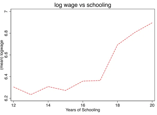
of their bounds on ∆(d+ 1, d) varies between (0; 0.226) and (0; 539). The lower bounds are just the result of the MTR assumption, the upper is the more important to analyze in their context. It is worth-noting that while the MTR would be a reasonable assumption to maintain in the returns to schooling literature, the MTS is debatable. As recognized by Manski and Pepper (2000), the MTS assumption fails in cases where ability and taste for schooling are potentially negatively associated, as discussed in Card (1994). A testable implication of the MTR-MTS assumption is that the mean observed wage must be non-decreasing in the number of years of schooling, more precisely E[Y|D=d] is monotone in
d. This testable implication can be tested using existing inference methods in Chetverikov (2013) or Hsu, Liu, and Shi (2018). As can be seen in Figure 1, in our case we observe some decreases. We implement the testing approach proposed by Hsu, Liu and Shi (2018) and reject the MTR-MTS testable implication. In this application, we will not assume either the MTS or the MTR. 6.2 6.4 6.6 6.8 7 (me a n ) lo g w a g e 12 14 16 18 20 Years of Schooling
log wage vs schooling
We recognize that the bounds proposed by Manski and Pepper (2000) may appear not that encouraging for empirical researchers, but this was a very early attempt. Since then we have improved our knowledge on the bounding approach and we will show that we can identify the sign of the treatment effect and obtain relatively reasonably informative bounds on the magnitude of the average returns to schooling using only the OTR assumption and our unconditional moment restrictions.
4.1. Data and Empirical context. We consider the data used by Ginther (2000). The data consists of a sample of white, employed males from the 1994 National Longitudi-nal Survey of Youth Geographic Micro-Data (NLSY). Our main outcome and endogenous variables of interest are the log weekly wage and the highest level of schooling completed, respectively. For a full description of the dataset and the sample under use, please refer to Ginther (2000).
We consider a school-quality characteristic proxied by teacher-pupil ratio as a poten-tial instrument, in the sense of the zero-covariance assumption for only the first moment, i.e. h(Z) = Z then Cov(Yd, Z) = 0. This variable has been initially considered as an
instrument (respecting the mean independence assumption) by Ginther (2000), motivated by some references therein. When using this variable, she showed that the Manski (1990, 1994) bounds cross, revealing that the mean independence assumption was too stringent for the teacher-pupil ratio instrument. We redo the test using more recent inferential methods like Chernozhukov, Kim, Lee, and Rosen (2015) and find the same result as Ginther (2000). However, notice that the mean independence can be rejected only because of some specific tail dependence between the instrument and the potential outcomes. For instance, as dis-cussed in Dearden et al. (2002), the dependence between the school-quality proxies and the potential outcomes can be explained by at least two main facts: (i) parents with greater interest in their child’s education and with higher earnings may choose to live or move to districts with better observed school-quality proxies. These children with such concerned and active parents may benefit from family environments that may enhance their talents, and thus their potential future earnings. We may therefore have people in the upper tail of the potential earnings distribution that are more likely to have been enrolled in schools with high values of school-quality proxies; (ii) Economically disadvantaged populations or regions often receive higher government grants that are often invested to improve school-quality proxies. However, the deprived neighborhoods and environments may negatively affect kids’ future potential earnings. Therefore, we may also have people in the lower tail of the potential earnings distribution likely to have been enrolled in schools that have high
values of school-quality proxies. These two facts are consistent with the idea that the in-validity of the mean independence is mainly driven by the observations from the upper or lower tail of the potential earnings distributions and there may not exist clear dependence patterns between middle class potential earnings and school-quality proxies.10 Usually tail dependence is captured by higher order moments that we will not use here. Interestingly, surveying the large applied literature that studies the relationship between school quality and earnings, Betts (2010) states:
“The entire body of work appears to agree that the relation between school resources and earnings of adults ranges between none and small but positive. Even the most positive results, based on studies that measure spending per pupil based on each worker’s state of birth, suggest an internal rate of return far below the rate of return to an extra year of high school or university, and below the real rate of interest.” In addition, the few works that find small correlations as in Dearden et al. (2002) did so only for females with low ability.
We therefore think that using only the first moment of the instrument is a reasonable assumption to maintain. In any case, if this assumption is too stringent, our bounds will cross, otherwise we could not reject the validity of this assumption based on the data in hand.
4.1.1. Methodology. In our sample under study, the highest level of schooling completed varies between 12 and 20. See Tables 1 and 2 in Appendix B for the summary statistics. We construct the confidence region for the ATEs, ∆(12 +s,12), s ∈ {1, ...,8} under the OTR assumption. Because we maintain the OTR assumption, we implement Algorithm 3 in Appendix A with the “clrtest” command and the “local linear” method. We use the default choices of bandwidth and kernel function recommended by Chernozhukov, Kim, Lee, and Rosen (2015, page 31). Since the theoretical support of the log wage is indeed unbounded, and also to avoid the bounding results being too sensitive to outliers, Ginther (2000) proposed to map the observed wage to a trimmed wage in the following way:
˜ Yi= QYτ ifYi ≤QYτ, Yi ifQYτ < Yi< QY1−τ, QY1−τ ifYi > QY1−τ,
10Notice that (i) and (ii) could suggest a U-relationship between the school-quality proxies and the
potential earnings. In such a context, we could not pretend that the IV has a monotone effect on the potential earnings. Then we could not use the monotone IV approach developed by Manski and Pepper (2000).
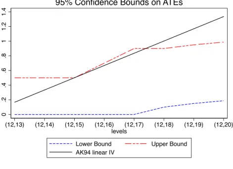
where QYτ is the τ-quantile of the observed wage.11 We follow Ginther (2000) and use this same transformation. Figure 2 depicts the 95% confidence regions for the ATEs: ∆(12 +
s,12), s∈ {1, ...,8}and this for different levels of trimming: τ = 5%,10% using the teacher-pupil ratio instrument. The dashed lines represent the lower and upper confidence bounds. The solid line represents the point estimates of the ATEs, ∆(12 +s,12), s ∈ {1, ...,8}
according the linear IV model used in Ashenfelter and Krueger (1994) discussed earlier.12 Tables 3 and 4 relegated to Appendix B present the exact values of our confidence regions. 4.1.2. Results and Interpretation. The results could be summarized as follows: (i) First, in all cases, the signs of all the ATEs, ∆(12 +s,12), s ∈ {1, ...,8} are always identified and non-negative. (ii) Second, while we reject the hypothesis that the ATEs: ∆(13,12), ∆(14,12), and ∆(15,12) are negative, we cannot reject the hypothesis that they are zero. It is worth noting that these treatment effects represent the treatment effect of dropping out of college versus being a high school graduate. These results are not surprising given the shape of the mean observed wage in Figure 1. The mean observed wage does not show any wage advantage for college dropouts even in presence ofa priori positive selection bias for any additional year of education. In contrast, we observe some small decreases at 13 and 15 years of education compared to 12 years of education. Furthermore, because both the upper and lower bounds for ∆(13,12), ∆(14,12), and ∆(15,12) are almost the same, we have no evidence that dropping out from college at 15 instead of 14 or 13 confers any additional wage returns. However, we observe a clear change in the upper bound at 16 years of education, which corresponds to the college graduates (those who have completed their college diploma) which appears in both Figures 2(a) and 2(b). In the latter figure, the lower bound for ∆(16,12) even becomes strictly positive. Starting from 16 years of education, both the lower and upper bounds tend to increase at each year, especially in Figure 2(b). These results are consistent with the “sheepskin effects” in the returns to education. Based on the screening theory of education, the sheepskin effects in the returns to education suggest that individuals with more schooling tend to earn more not because (or not only because) schooling makes them more productive, but rather because it signals them as more productive. This theory therefore predicts thatpotential wages should rise faster with extra years of education when the extra year also conveys a certificate. See Hungerford and Solon
11Lee (2009) also considers a transformation of the observed outcome for his application.
12We do not plot the confidence regions for this latter since their estimates are very precise, i.e., ∆(d+
1, d)=0.167 (± 0.0003) so that the confidence intervals are very close to the line already depicted in the graph.
0 .2 .4 .6 .8 1 1.2 1.4 (12,13) (12,14) (12,15) (12,16) (12,17) (12,18) (12,19) (12,20) levels
Lower Bound Upper Bound
AK94 linear IV
95% Confidence Bounds on ATEs
(a)Trimming Levelτ= 5%
0 .2 .4 .6 .8 1 1.2 1.4 (12,13) (12,14) (12,15) (12,16) (12,17) (12,18) (12,19) (12,20) levels
Lower Bound Upper Bound
AK94 linear IV
95% Confidence Bounds on ATEs
(b)Trimming Levelτ= 10%
(1987), Belman and Heywood (1991), and Jaeger and Page (1996) for a detailed discussion on the evidence of sheepskin effects in the US. Notice that, in our case, any additional year of education starting from 16 would confer a certificate to some individuals in the sample depending on the length of a masters degree —that varies between 1 and 2 years— and a Ph.D which would be conferred at least 3 years or more after college graduation, depending on the fields. This could explain why we observe some changes in either the upper or lower bounds at each additional year of schooling after college graduation. (iii) While some evidence of the presence of sheepskin effects in returns to education in US has been discussed in the above cited papers, for some unclear reasons, the empirical literature has mainly focused on the linear IV model which by construction assumes away any potential sheepskin effect. Indeed, unlike the potential outcome model we entertain here that is consistent with all potential non-linearity in the wage equation, the linear IV model by construction does not allow for the possibility of a discontinuity in the functional form at the year of schooling that confers a diploma. This linearity imposes a very strong restriction on the data and may often lead to misleading interpretations. For instance, according to the linear IV estimates of the yearly returns to education we surveyed earlier, the returns to schooling of college dropouts versus high school graduates are estimated to be strictly positive, varying between ∆(d+s,12) = 0.060×sand ∆(d+s,12) = 0.167×sfors= 1,2,3. However, this may be due to a misspecification issue in which the researcher tries to fit a discontinuous piecewise function where positive jumps appear only on the schooling year that delivers a certificate, as suggested by the screening theory of education. We also see that the magnitude of our bounds are informative enough to reject various linear IV point estimates found in the literature; for instance, the Ashenfelter and Krueger (1994) point estimates fall outside our confidence regions. More precisely, for the data under use, Figure 2(a) (resp. 2(b)) suggests that any linear estimates of the returns to education must be lower than 0.123 (resp. 0.1075). (iv) Finally, it is worth noting that in the presence of sheepskin effects, the ACR estimand must be interpreted with a lot of caution to avoid misleading predictions. Indeed, since it is a weighted average, it could overvalue the causal effect of dropping out of college and undervalue the impact of graduation. Moreover, the weight should be analyzed more carefully than it is commonly done, because if we have more college droppouts than college graduates, the ACR could be less informative (if not non-informative at all) about the causal effect of college graduation and vice-versa. Overall, we think that over-simplified models (like the linear IV model) may rule out by construction some potential relevant economic models, like sheepskin effects, and some over-simplified estimators like 2SLS may not necessarily capture the causal parameter of interest. We think that the
partial identification approach that we entertain here could be general enough to avoid (by construction) ruling-out some relevant theories that are potentially more compatible with the data and at the same time could provide informative bounds to discriminate between various potential specifications.
5. Conclusion
In this paper, we propose a novel approach to derive sharp bounds on various treatment effect parameters using only a finite set of unconditional moment restrictions. To show the sharpness of our bounds, we appeal to the convex analysis literature. From a practical point of view, our method is useful in empirical applications where the commonly invoked IV mean independence restriction is too stringent of a requirement and incompatible with the data. We revisited Ginther’s (2000) returns to schooling application using our bounding approach and derive informative bounds on average returns to schooling. Our results are consistent with sheepskin effects in the returns to education literature. However, our sample is not large enough and does not contain enough disaggregated information on the exact year each individual obtained a certificate, which would be required for a deeper analysis of the sheepskin effects using our bounding approach. We therefore leave the full exploration of this question for future research.
AppendixA. Additional Results: Zero-Covariance and OTR.
Consider that the OTR assumption holds and assume thatE[h(Z)] = 0. OTR can be viewed as the union of M T R+ (d > d0 ⇒Yd≥Yd0 a.s) andM T R−(d > d0 ⇒Yd≤Yd0 a.s). Notice that theM T R+ implies that for all non-decreasing integrable function g(.), we have
d > d0⇒g(Yd)≥g(Yd0) a.s. (A.1) For instance, we can considerg(Yd) =Ydorg(Yd) = 1{Yd> y}. ImposingM T R+mainly affects the previous bounds
we derived on the unobserved counterfactuals, i.e., Eg(Yd)(1 +λ0h(Z))1[D 6=d]
. To ease the exposition, we use the shorthand notationδ≡1 +λ0h(Z) and then under theM T R+we have the following bounds on the unobserved counterfactuals: E h 1[D > d] min{δg(Y), δg d}+1[D < d] min{δg(Y), δgd} i ≤Eg(Yd)δ1[D6=d] ≤ (A.2) E h 1[D > d] max{δg(Y), δg d}+1[D < d] max{δg(Y), δgd} i . Then, we have E h δg(Y)1[D=d] +1[D > d] min{δg(Y), δg d}+1[D < d] min{δg(Y), δgd} i ≤Eg(Yd)] ≤ (A.3) E h δg(Y)1[D=d] +1[D > d] max{δg(Y), δg d}+1[D < d] max{δg(Y), δgd} i .
for allλ∈Rm. Similarly, underM T R−we can show that E h δg(Y)1[D=d] +1[D < d] min{δg(Y), δg d}+1[D > d] min{δg(Y), δgd} i ≤Eg(Yd)] ≤ (A.4) E h δg(Y)1[D=d] +1[D < d] max{δg(Y), δg d}+1[D > d] max{δg(Y), δgd} i . for allλ∈Rm. Denote by ˜Θ+d,d0 (resp. ˜Θ −
d,d0) theouter setof the joint parameters (θd, θd0) under Assumptions 1, 2, andM T R+ (resp. M T R−). We call them the outer set instead of the identified set because we will not show here their sharpness even if we conjecture that they are sharp. By generalizing the above bounds whenE[h(Z)] 6= 0, we can derive the following characterization of the outer sets: Ford > d0,we have
˜ Θ+d,d0≡
(
(θd, θd0)∈[g
d, gd]×[gd0, gd0] such thatθd≥θd0 and (∗)0≤ inf (γ,λ)∈Sm+1 E(γ+λ0h(Z))g(Y)1[D=l] +1[D > l] max{(γ+λ0h(Z))g(Y),(γ+λ0h(Z))gl} +1[D < l] max{(γ+λ0h(Z))g(Y),(γ+λ0h(Z))gl} −θl(γ+λ0h(Z)) , for l ∈ {d, d0} ) (A.5) and ˜ Θ−d,d0 ≡ ( (θd, θd0)∈[g
d, gd]×[gd0, gd0] such thatθd≤θd0 and (∗∗)0≤ inf (γ,λ)∈Sm+1E (γ+λ0h(Z))g(Y)1[D=l] +1[D < l] max{(γ+λ0h(Z))g(Y),(γ+λ0h(Z))g l} +1[D > l] max{(γ+λ0h(Z))g(Y),(γ+λ0h(Z))gl} −θl(γ+λ0h(Z)) , for l ∈ {d, d0} ) . (A.6)
Therefore, the outer set for (θd, θd0) under the OTR assumption is ˜
Θd,d= Θ+d,d0∪Θ −
d,d0.
Notice that we are in presence of what is called an intersection-union test (Berger, 1982) widely used in Bioequiv-alence hypotheses. Theorem 1 of Berger and Hsu (1996) showed that the construction of 1−αconfidence regions
CIn,+1−α(d, d0), andCI− n,1−α(d, d0) such thatP(CI + n,1−α(d, d0)⊇Θ + d,d0)≥1−αandP(CIn,−1−α(d, d0)⊇Θ − d,d0)≥1−α ensures to haveP(CIn,+1−α(d, d 0)∪CI− n,1−α(d, d 0)⊇Θ
d,d0)≥1−α. In other words, the Theorem 1 of Berger and Hsu (1996) means that if each of the individual tests is performed at levelα, then the overall test also has the same level. There is no need for multiplicity adjustment for performing multiple tests. We therefore propose the following algorithm to construct a valid confidence region forθd−θd0 ford > d0.
Algorithm 3. (Implementation usingcmi-test/clrtest)
Step 1. Draw auxiliary i.i.d. samples (Vi, Wi)ni=1from distributionFV,Windependent of data samples{Yi, Zi, Di}ni=1. Step 2. Letφ+(θ
d, θd0, α,{Yi, Zi, Di, Vi, Wi}ni=1)∈ {0,1}(resp. φ −(θ
d, θd0, α,{Yi, Zi, Di, Vi, Wi}ni=1)∈ {0,1}) be the result of the Stata commandcmi-testorclrtestimplemented to test the null hypothesis:
H0+: θd≥θd0 satisfies (∗) vs Ha+:θd≥θd0 doesn’t satisfy (*)
resp. H−0 : θd≤θd0 satisfies (∗) vs Ha−:θd≤θd0 doesn’t satisfy (**)
with nominal level 1−αand data observation{Yi, Zi, Di, Vi, Wi}ni=1}.
Step 3. If the null hypothesis H0 (resp. H˜0) is rejected, let φ+(θd, θd0, α,{Yi, Zi, Di, Vi, Wi}ni=1) = 1 (resp.
φ+(θ
Step 4. Construct the level 1−αconfidence interval for (θd−θd0) as follows CIn,1−α(d, d0)≡ n θd−θd0: (θd, θd0)∈[gd, gd]×[gd0, gd0], φ+(θd, θd0, α,{Yi, Zi, Di, Vi, Wi}ni=1) = 0 andφ−(θd, θd0, α,{Yi, Zi, Di, Vi, Wi}ni=1) = 0 o .
AppendixB. Summary Statistics and Results
Table 1. Summary Statistics
Total
Observations 874
log wage 6.3886 (0.4649) years of schooling 14.5709 (2.5851) Teacher-to-pupil ratio 0.0543 (0.0128)
Average and standard deviation (in the parentheses)
Table 2. Empirical distribution of years of schooling
Years of schooling (D) Observations P(D=d)
12 332 0.3799 13 66 0.0755 14 61 0.0698 15 47 0.0538 16 194 0.2220 17 51 0.0584 18 41 0.0469 19 15 0.0172 20 67 0.0767 Total 874 1
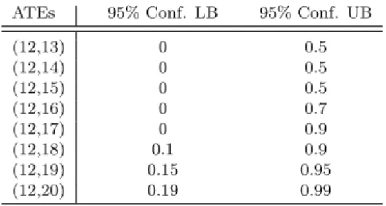
Table 3. Confidence bounds on ATEs for τ = 5% trimming
ATEs 95% Conf. LB 95% Conf. UB
(12,13) 0 0.5 (12,14) 0 0.5 (12,15) 0 0.5 (12,16) 0 0.7 (12,17) 0 0.9 (12,18) 0.1 0.9 (12,19) 0.15 0.95 (12,20) 0.19 0.99
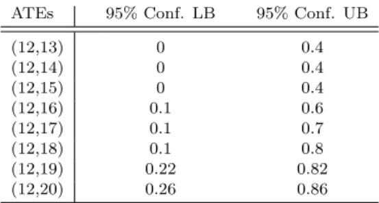
Table 4. Confidence bounds on ATEs forτ = 10% trimming
ATEs 95% Conf. LB 95% Conf. UB
(12,13) 0 0.4 (12,14) 0 0.4 (12,15) 0 0.4 (12,16) 0.1 0.6 (12,17) 0.1 0.7 (12,18) 0.1 0.8 (12,19) 0.22 0.82 (12,20) 0.26 0.86
conf. LB (UB) stands for confidence lower (upper) bound.
AppendixC. Proof of the main results
C.1. Proof of Theorems 1 and 2. We will start by proving Theorem 2, and then we will show in C.1.2 that Theorem 1 is a special case of Theorem 2 under the normalizationEh(Z) = 0. Before doing so, let’s provide a formal
definition of the identified set in our context.
Definition 2 (Identified Set). Given Assumption 1 and 2, define the identified set ΘI of (E[g(Y0)], ...,E[g(YT)])
as the set of all (θ0, ..., θT)for which there exists random variable (G0, ..., GT) such that the joint distribution of
(Y, Z, D, G0, ..., GT)satisfy the following conditions:
(1) EGd=θd,∀d∈ D,
(2) E[(Gd−θd)·h(Z)] = 0∀d∈ D,
(3) P(Gd = g(Y)|D = d) = 1 and P(Gd ∈ Γd|D 6= d) = 1, where Γd ≡ Supp(g(Yd)|D = d), and gd ≡
inf Γd, gd≡sup Γd,∀d∈ D.
C.1.1. Proof of Theorem 2. We first show (θ0, ..., θT)∈ΘIimplies inequality (2.11) for eachd∈ D. Let (θ0, ..., θT)
be any point in ΘI, and let (G0, ..., GT) be random variables satisfying Condition (1)-(3) in Definition 2. Condition
(1) and (2) imply, for anyd∈ D, any (γ, λ)∈ Sm+1
0 =E(Gd−θd)(γ+λ0h(Z)).
Combining the above equality with Condition (3), we know that: 0≤ inf (γ,λ)∈Sm+1E h 1(D=d)(g(Y)−θd)(γ+λ0h(Z)) +1(D6=d) sup y∈Γd n (y−θd)(γ+λ0h(Z)) oi By the definition ofg
dandgd, we can rewrite the above inequality as
0≤ inf (γ,λ)∈Sm+1E " 1(D=d)(g(Y)−θd)(γ+λ0h(Z)) +1(D6=d) max y∈{gd,gd} n (y−θd)(γ+λ0h(Z)) o # .
which is equivalent to inequality (2.11).
Next, we show when (θ0, ..., θT) satisfies inequality (2.11), then (θ0, ..., θT) ∈ ΘI. Let (θ0, ..., θT) be a point
satisfying inequality (2.11) ford∈ D. Then, we want to construct random variables (G0, ..., GT) which satisfy all
conditions in Definition 2. To do so, define
ϕd(Y, D, Z;γ, λ) ≡ fd(Y, D, γ+λ
0h(Z))−θ
d(γ+λ0h(Z))
Recall that fd(Y, D, γ+λ 0 h(Z))≡1[D=d](γ+λ0h(Z))g(Y) +1[D6=d] max (γ+λ0h(Z))gd,(γ+λ0h(Z))gd .
Using these notation, inequality (2.11) can be written as 0≤inf{ϕd(γ, λ) : (γ, λ)∈ Sm+1}. Note thatϕd(Y, D, Z;γ, λ)
is linearly homogeneous in (γ, λ). That is, for anyα >0, we have
ϕd(Y, D, Z;αγ, αλ) =α·ϕd(Y, D, Z;γ, λ).
Therefore, for any (γ, λ)∈Rm+1with 0<k(γ, λ)k, we have ϕd(γ, λ)≥0 ⇔ k(γ, λ)kϕd γ k(γ, λ)k, λ k(γ, λ)k ≥0 ⇔ ϕd γ k(γ, λ)k, λ k(γ, λ)k ≥0,
Sincek(γ,λγ)k,k(γ,λλ)k∈ Sm+1, we know that 0≤inf{ϕd(γ, λ) : (γ, λ)∈ Sm+1}is equivalent to 0≤inf{ϕd(γ, λ) :
(γ, λ)∈Rm+1\ {0}}. Sinceϕd(0,0) = 0 for anyθd, we also know that 0≤inf{ϕd(γ, λ) : (γ, λ)∈ Sm+1}is equivalent to 0≤inf{ϕd(γ, λ) : (γ, λ)∈Rm+1}.
Now, notice thatϕd(γ, λ) is a convex function of (γ, λ) mapping fromRm+1toR, so that its subgradient always
exists. Also, since inequality (2.11) is equivalent to 0≤inf{ϕd(γ, λ) : (γ, λ)∈Rm+1}andϕd(0,0) = 0, the infimum
is always achieved atγ= 0 andλ= 0. This implies 0∈∂ϕd(0,0), where∂ϕd(0,0) stands for the partial subgradient
ofϕdat pointγ= 0 andλ= 0. Let∂ϕd(Y, D, Z; 0,0) denotes the subgradient ofϕd(Y, D, Z;γ, λ) at pointγ= 0 and
λ= 0. Then, Proposition 2.2 in Bertsekas (1973) and 0∈∂ϕd(0,0) implies, there exists a measurable functionψd(·)
such thatEψd(Y, D, Z) = 0 andψd(Y, D, Z)∈∂ϕd(Y, D, Z; 0,0) almost surely. We can show that
∂ϕd(Y, D, Z; 0,0) =
[1(D=d)g(Y) +1(D6=d)x−θd]·(1, h(Z))0:x∈[gd, gd]
where (1, h(Z)) stands for a vector inRm+1whose first element is 1 and the rest element ish(Z).
Letψ(1)d (Y, D, Z) denote the first dimension inψd(Y, D, Z). LetQbe a random variable, distributed as uniform
distribution in [0,1] and is independent of (Y, D, Z). Construct functionGd(Y, D, Z, Q) as the following
Gd(Y, D, Z, Q) = g(Y) ifD=d, gd ifD6=d, andQ≤(gd−g d) −1 ψ(1) d (Y, D, Z) +θd−gd g d if otherwise (C.1)
and then defineGd(Y, D, Z)≡E[Gd(Y, D, Z, Q)|Y, D, Z].
By the construction ofGd(Y, D, Z), we have Condition (3) in Definition 2 satisfied and it can be shown that
(Gd(Y, D, Z)−θd)·(1, h(Z))0=ψd(Y, D, Z) almost surely.
Notice that since ψd(Y, D, Z) = g(Y) when D = d, the above equality obviously holds whenD = d. To see
that it also holds whenD6=d, remark that the independence between Q and (Y, D, Z) implies that (Gd(Y, D, Z)−
θd) =ψ
(1)
d (Y, D, Z) when D 6= d. Moreover, since ψd(Y, D, Z) ∈ ∂ϕd(Y, D, Z; 0,0) we know thatψd(Y, D, Z) =
ψ(1)d (Y, D, Z)·(1, h(Z))0whenD6=d.
Therefore sinceEψd(Y, D, Z) = 0, we haveEGd(Y, D, Z) = θd and E(Gd(Y, D, Z)−θd)h(Z) = 0, which then