This is an author produced version of
Nonlinear unsteady streaks engendered by the
interaction of free-stream vorticity with a compressible boundary layer
.
White Rose Research Online URL for this paper:
http://eprints.whiterose.ac.uk/113951/
Article:
Marensi, E., Ricco, P. and Wu, X. (2017) Nonlinear unsteady streaks engendered by the
interaction of free-stream vorticity with a compressible boundary layer. Journal of Fluid
Mechanics, 817. pp. 80-121. ISSN 0022-1120
https://doi.org/10.1017/jfm.2017.88
promoting access to
White Rose research papers
[email protected] http://eprints.whiterose.ac.uk/
Nonlinear unsteady streaks engendered by
the interaction of free-stream vorticity with
a compressible boundary layer
Elena Marensi
1,2
†
, Pierre Ricco
1and Xuesong Wu
31
Department of Mechanical Engineering, The University of Sheffield, S1 3JD Sheffield, UK
2
Department of Fluid Dynamics, A*Star Institute of High Performance Computing, Singapore
3
Department of Mathematics, Imperial College London, SW7 2AZ London, UK (Received 28 February 2017)
The nonlinear response of a compressible boundary layer to unsteady free-stream vortical fluctuations of the convected-gust type is investigated theoretically and nu-merically. The free-stream Mach number is assumed to be of O(1) and the effects of compressibility, including aerodynamic heating and heat transfer at the wall, are taken into account. Attention is focused on low-frequency perturbations, which induce strong streamwise-elongated components of the boundary-layer disturbances, known as streaks or Klebanoff modes. The amplitude of the disturbances is intense enough for nonlinear interactions to occur within the boundary layer. The generation and nonlinear evolu-tion of the streaks, which acquire anO(1) magnitude, are described on a self-consistent and first-principle basis using the mathematical framework of the nonlinear unsteady compressible boundary-region equations, which are derived herein for the first time. The free-stream flow is studied by including the boundary-layer displacement effect and the solution is matched asymptotically with the boundary-layer flow. The nonlinear inter-actions inside the boundary layer drive an unsteady two-dimensional flow of acoustic nature in the outer inviscid region through the displacement effect. A close analogy with the flow over a thin oscillating airfoil is exploited to find analytical solutions. This anal-ogy has been widely employed to investigate steady flows over boundary layers, but is considered herein for the first time for unsteady boundary layers. In the subsonic regime the perturbation is felt from the plate in all directions, while at supersonic speeds the disturbance only propagates within the dihedron defined by the Mach line. Numerical computations are performed for carefully chosen parameters that characterize three prac-tical applications: turbomachinery systems, supersonic flight conditions and wind tunnel experiments. The results show that nonlinearity plays a marked stabilizing role on the velocity and temperature streaks, and this is found to be the case for low-disturbance environment such as flight conditions. Increasing the free-stream Mach number inhibits the kinematic fluctuations but enhances the thermal streaks, relative to the free-stream velocity and temperature respectively, and the overall effect of nonlinearity becomes weaker. An abrupt deviation of the nonlinear solution from the linear one is observed in the case pertaining to a supersonic wind tunnel. Large-amplitude thermal streaks and the strong abrupt stabilizing effect of nonlinearity are two new features of supersonic flows. The present study provides an accurate signature of nonlinear streaks in compressible boundary layers, which is indispensable for the secondary instability analysis of unsteady streaky boundary-layer flows.
Key words:compressible boundary layers, transition to turbulence † Email address for correspondence: [email protected]
1. Introduction
The transition from a laminar to a turbulent state in boundary layers, although studied for over a century, still represents one of the outstanding unsolved problems in fluid mechanics. A thorough understanding of the physics underlying this phenomenon is of great importance from a fundamental as well as from a practical point of view. The wall shear stress and heat transfer characteristics change dramatically depending on the flow regime being laminar, transitional or turbulent. Therefore, quantitative prediction and control of transition play a decisive role in determining the operating conditions and performance of flows around high-speed airfoils in a variety of industrial applications. Relevant examples are commercial and high-speed aircraft, space capsule re-entry into the atmosphere and flows around turbine stator vanes or rotor blades.
Boundary-layer transition is known to be strongly influenced by disturbances present in the oncoming stream, which penetrate into the boundary layer and eventually lead to the breakdown of the laminar flow. Such perturbations consist of acoustic (pressure), kinematic (vortical) and entropy (temperature) fluctuations, and may exist independently of each other when they are of sufficiently small amplitude.
In this paper we are concerned with free-stream vortical perturbations whose intensi-ties are high enough (T u=1% or more, where T u is the root-mean-square value of the velocity fluctuations) for transition to occur rather early, bypassing the so-called orderly route via viscous Tollmien-Schlichting (T-S) waves. In this scenario, referred to as by-pass transition (Morkovin 1984), the laminar boundary-layer breakdown is preceded and caused by unsteady streamwise-elongated regions of high and low streamwise velocity. These structures have been referred to as breathing modes (Taylor 1939) because of their resemblance to a thickening and thinning of the layer, Klebanoff modes (Kendall 1985) after the experiments of Klebanoff (1971), or laminar streaks. The focus of our work is on the generation and nonlinear evolution of streaks in the compressible regime because in high-speed flows transition occurs more frequently through the bypass route than via the T-S wave growth described by classical stability theory.
1.1. Experiments and direct numerical simulations
Experimental works (Arnal & Juillen 1978; Kendall 1985, 1990, 1991; Westinet al.1994, 1998; Matsubara & Alfredsson 2001; Franssonet al.2005) and direct numerical simula-tions (DNS) using realistic free-stream disturbances (Nagarajanet al.2007; Ovchinnikov
et al.2008; Brinkerhoff & Yaras 2015) have provided an overall picture of bypass tran-sition induced by free-stream turbulence in the incompressible regime. The reader is also referred to DNS studies (e.g. Jacobs & Durbin 2001; Brandt et al. 2004; Zaki & Durbin 2005) using inflow conditions synthesized through the continuous modes of the Orr-Sommerfeld/Squire equations. Despite its importance in high-speed aircraft design and turbomachinery applications, the literature available on bypass transition in com-pressible flows is more limited than for incomcom-pressible flows. Supersonic wind tunnel experiments (Laufer 1961; Pate & Schueler 1969; Kendall 1967; Schneider 2001) showed that the transition behaviour is dominated by the noise radiated from the turbulent boundary layers on the walls. Transition may occur earlier in laboratory experiments than in flight conditions because of the high levels of tunnel noise (Schneider 2001). This discrepancy prevents the direct use of laboratory data for high-speed vehicle design. Al-though most of the experimental studies in the last few decades have focussed on acoustic disturbances, it should be recognized that more attention needs to be devoted to vortical
disturbances. As speculated by Kendall (1975), at low speeds the tunnel sound might be less effective than other type of disturbances, such as the vortical fluctuations. In flight conditions vortical disturbances are the main source of perturbation influencing transi-tion, while acoustic modes are weak and only become relevant at locations affected by the noise radiated by the engine.
Mayeret al.(2011) performed DNS of the downstream development of a pair of oblique instability waves in a supersonic flat-plate boundary layer. They showed that transition in supersonic two-dimensional boundary layers can be initiated by very low disturbance levels (e.g. less than 0.01%), which explains the practical relevance of the oblique break-down mechanism for quiet environment such as free flight. Joo & Durbin (2012) carried out DNS of the transition initiated by discrete instability modes and continuous vor-tical modes in a Mach 4.5 boundary layer. As in Jacobs & Durbin (2001) and Zaki & Durbin (2005), their approach consisted of specifying the inflow conditions in terms of a superposition of the continuous spectra of the Orr-Sommerfeld and Squire operators. Such a practice has been questioned by Dong & Wu (2013) and Wu & Dong (2016), who showed that continuous spectra exhibit non-physical features (i.e. entanglement of Fourier components and abnormal size of the streamwise free-stream velocity) because non-parallel flow effects in the boundary layer are neglected. Non-parallelism actually plays a leading-order role in the entrainment of free-stream vortical disturbances into the boundary layer.
1.2. Theoretical works
In order to include the interaction between free-stream disturbances and the bound-ary layer, a rigorous mathematical formulation has been developed by Goldstein and co-workers (Goldstein et al.1992; Goldstein & Leib 1993; Goldstein 1997; Wundrow & Goldstein 2001). Goldstein’s theory is based on the boundary-region equations (Kemp 1951), which are the rigorous asymptotic limit of the Navier-Stokes equations for low-frequency and long-wavelength perturbations. For these disturbances, the streamwise derivatives in the viscous and pressure gradient terms are negligible, while the span-wise viscous diffusion is retained. In the limit of small-amplitude disturbances or short downstream distance, the boundary-region equations can be linearized about the Bla-sius solution. Leibet al. (1999) used the linearized unsteady boundary-region equations (LUBR) to investigate the response of an incompressible laminar boundary layer to free-stream unsteady vortical fluctuations of the convected-gust type. Wu & Luo (2003) and Wu & Choudhari (2003) studied the instability of a Blasius boundary layer in the pres-ence of steady and unsteady streaks, and showed that inviscid instability may occur when the distortion of the Klebanoff modes reaches a certain threshold value.
The linear analysis of Leibet al.(1999) was extended by Riccoet al.(2011) to include nonlinear effects. Nonlinearity was found to attenuate the amplification of the streaks and to distort the mean-flow profile significantly. A secondary instability analysis was carried out on the nonlinear streaks, proving that the streaky boundary layer may become inviscidly unstable during certain phases of the time modulation.
Ricco & Wu (2007) extended the incompressible analysis by Leibet al.(1999) to the compressible case and explained the formation and growth of thermal streaks, which are thought to play a significant role in the secondary instability. Riccoet al.(2009) and Ricco
et al.(2013) further studied the influence of wall heat transfer and wall suction, respec-tively, on the thermal streaks. The boundary-layer signature in the region relatively close to the leading edge corresponds to the inhomogeneous solution forced by the free-stream disturbance. However, Ricco & Wu (2007) also observed that sufficiently downstream exponentially growing disturbances are formed. For high subsonic and supersonic Mach
numbers, the appearance of the amplifying disturbances was in the streamwise region of practical interest. Ricco & Wu (2007) showed that the growing disturbances evolved from the so-called quasi-three-dimensional Lam-Rott eigensolutions, which are excited by the free-stream disturbance and may be identified as highly oblique low-frequency T-S waves in the so-called first-mode family (Mack 1975, 1984). Riccoet al.(2009) found that wall cooling suppresses the streaks and enhances the growth of the instability waves.
The parabolized-stability equations (PSE) approach has been developed and used to study the evolution of instability modes in compressible boundary layers (see e.g. Chang
et al.1991). This methodology is based on the assumption that the base flow varies slowly in the streamwise direction and thus a Wentzel-Kramers-Brillouin (WKB) type of analy-sis is employed to parabolize the Navier-Stokes equations. The method requires, however, anad hociterative procedure to identify a local streamwise wavenumber, and, further-more, the presence of the streamwise pressure gradient causes some numerical instability due to a residual ellipticity in the equations (Li & Malik 1996). Neither of these problems occurs in the boundary-region equation approach because the local streamwise wavenum-ber tends to zero in the low-frequency asymptotic limit, and the equations are strictly parabolic. It should be pointed out that what we referred to as the boundary-region equa-tion approach consists of appropriate initial (upstream) and boundary condiequa-tions, which correctly describe the entrainment of physically realizable free-stream disturbances. This is in contrast to the so-called optimal perturbation theory (Anderssonet al.1999; Zuccher
et al.2006), which uses the adjoint of the boundary-region equations or of the PSE to find the initial (upstream) disturbances that undergo the maximum gain when evolving to a pre-selected streamwise location. Free-stream disturbances, the very factor causing bypass transition, are not taken into account in the latter formulation.
1.3. Objectives
As in the incompressible case, bypass transition in compressible boundary layers is of relevance for engineering applications, but it is also challenging theoretically because of both the difficult mathematics involved and the complex physical mechanisms at play. As an essential step towards understanding and predicting compressible bypass transi-tion, we formulate a rigorous description of the formation and nonlinear development of the unsteady compressible streaks induced by free-stream vortical fluctuations. Such a mathematical theory for compressible disturbances responsible for bypass transition is still absent. A further goal is to explain the nonlinear interactions between the free-stream flow and the viscous boundary-layer flow, which occur through the displacement effect.
In §2, the mathematical formulation and the scalings adopted are presented. In §2.1 the free-stream perturbation is described and in §2.2 the nonlinear unsteady compressible boundary-region equations are derived. In §2.3 the outer-flow solution is obtained and matched with the inner solution in §2.4. The numerical procedure to solve the boundary-region problem is outlined in §3. The outer-flow velocity and pressure fields are shown in §4 for the subsonic and supersonic regimes. In §5.1 three different cases are considered, i.e. a turbomachinery flow (§5.1.1), a free flight flow (§5.1.2) and a supersonic wind tunnel flow (§5.1.3). The relevant results for the unsteady compressible streaks are presented in §5.2 and §5.3. A summary and conclusions are given in §6.
2. Formulation: scalings and governing equations
An air flow with a mean uniform velocityU∗∞and constant temperatureT∞∗ is consid-ered; hereinafter the symbol∗ is used to indicate dimensional quantities. Superimposed
on the mean flow are homogeneous, statistically stationary turbulent vortical fluctua-tions, which are of the convected-gust type, i.e. they are passively advected byU∗
∞. The oncoming flow is considered isentropic and air is treated as a perfect gas. The speed of sound in the free stream is:
a∗
∞=
p
γR∗T∗
∞, (2.1)
where γ=1.4 is the ratio of the specific heats and R∗ is the universal gas constant (R∗=287.05 N m kg−1K−1). The Mach number is defined as
M∞≡ U∗ ∞ a∗ ∞ =O(1). (2.2)
In the Cartesian coordinate system employed to describe the flow, a point is repre-sented by a position vectorx∗=x∗i+y∗j+z∗k, wherex∗,y∗ andz∗ define the stream-wise, wall-normal and spanwise directions, respectively. The spatial coordinates are non-dimensionalized by a suitable reference length scaleλ∗, which we shall specify below. The velocity and temperature reference scales areU∗
∞andT∞∗. The fluid properties, such as the densityρ∗and the dynamic viscosityµ∗, are scaled by their respective constant free-stream values,ρ∗
∞ andµ∗∞. The timet∗ and the pressurep∗ are non-dimensionalized by
λ∗/U∗
∞ andρ∗∞U∞∗2, respectively.
It should be pointed out that in the supersonic regime shocks appear when the aero-dynamic body (including a flat plate) has a finite thickness, and that at sufficiently high Mach numbers shocks can also arise for the idealized case of a flat plate with zero thick-ness due to the significant displacement produced by the viscous boundary-layer motion near the leading edge. The presence of a shock may change the boundary-layer instability properties if it is sufficiently close to the boundary layer (Chang et al.1990; Cowley & Hall 1990). Moreover, when any of the three types of perturbations, e.g. a vortical fluctua-tion, interacts with a shock, all three disturbances may appear downstream of the shock (McKenzie & Westphal 1968). The acoustic and entropy perturbations may influence transition via receptivity mechanisms (Fedorov & Khokhlov 2003; Zhong & Wang 2012; Qin & Wu 2016). In the present study, effects of shocks are neglected on the grounds that the plate is sufficiently thin and the Mach number is moderate so that shocks are weak and distant from the boundary. In this case, the interaction of unsteady distur-bances with the shock is decoupled from their subsequent interaction with the boundary layer (Qin & Wu 2016). The response of the boundary layer to each type of free-stream disturbance downstream of a shock can be analysed separately.
2.1. Free-stream disturbances and scaling
Free-stream turbulence is in general of broadband nature. For simplicity, we consider the case of vortical perturbation consisting of a pair of vortical modes with the same frequency (and hence streamwise wavenumber), but opposite spanwise wavenumber±k∗
z.
In the incompressible analysis of Riccoet al.(2011), this choice of free-stream disturbance has led to good quantitative agreement between the theoretical prediction and wind tunnel experimental data. A similar behaviour is expected in the compressible case. The formulation and computation can be extended to realistic free-stream perturbations, which are of broadband nature as was shown by Zhanget al.(2011) for incompressible flows.
The velocity field of free-stream convected gusts of the assumed form can be expressed as u−i=ǫu∞(x−t, y, z) =ǫ uˆ∞+eikzz+uˆ∞ −e−ikzz eikx(x−t)+ikyy+c.c., whereˆu∞
perturbation level andc.c.indicates the complex conjugate. From the continuity equation, it follows that
kxuˆ∞x,±+kyuˆy,∞±±kzuˆ∞z,±= 0. (2.3) It is appropriate and convenient to take λ∗=1/k∗
z, so that kz=1. The characteristic
Reynolds number is Rλ≡ U ∗ ∞λ∗ ν∗ ∞ ≫1. (2.4)
Only the components of the free-stream disturbance withkx≪1 are considered as they
have been shown in experiments to be the ones that can penetrate the most into the boundary layer to form streaks.
According to the result of Leibet al. (1999), the velocity perturbation is maximum whenx=O(k−1
x ). The following scaling is thus introduced:
¯
x≡kxx=O(1). (2.5)
As a measure of the ratio between the boundary-layer thickness δ∗ and the spanwise length scaleλ∗ at ¯x=O(1), a scaled spanwise wavenumber is defined as
κ≡ 1 λ∗ s λ∗ xν∞∗ 2πU∗ ∞ = √kz kxRλ . (2.6)
The interest is in the downstream viscous region whereδ∗=
O(λ∗) so that viscous diffu-sion effects in the spanwise and wall-normal directions are comparable. This occurs at streamwise locationsx∗=
O(λ∗R
λ), which, together with (2.5), leads tokx=O(R−λ1), or,
equivalently,κ=O(1). As shown by Leibet al.(1999),O(ǫ) free-stream disturbances can produceO(ǫ/kx) fluctuations of the streamwise velocity component within the boundary
layer. Nonlinear effects become of leading order whenǫ/kx=O(1), i.e. when the turbulent
Reynolds number
rt≡ǫRλ=O(1), (2.7)
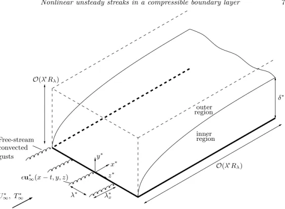
sincekx=O(R−λ1). A schematic illustration of the flow domain and its asymptotic
struc-ture is shown in figure 1.
2.2. The inner region: nonlinear unsteady compressible streaks
In the boundary layer the solution is expressed as the superimposition of the unsteady perturbation on the steady laminar compressible boundary layer. The velocities and temperature of the Blasius flow have the similarity solution (Stewartson 1964)
{U, V}= F′(η),T(ηcF′−F) √ 2xRλ , T =T(η),
where the prime indicates differentiation with respect to the similarity variableη,
η≡ r Rλ 2x Z y 0 ρ(x,yˇ) dˇy, andηc=T−1 Z η 0
T(ˇη) dˇη. Thex-momentum and the energy equations are:
F F′′+µ TF ′′′= 0, µT′ T ′ + PrF T′+ Pr(γ −1)M∞2 µ TF ′′2= 0,
Free-stream convected gusts λ∗ ǫu∗ ∞(x−t, y, z) outer inner region region U∗ ∞, T ∗ ∞ δ∗ O(λ∗ Rλ) O(λ∗ Rλ) λ∗ x x∗ y∗ z∗
Figure 1: Sketch of the flow configuration representing the asymptotic regions (adapted from Leibet al.1999).
where the Prandtl number Pr=0.7. The system is subject to the boundary conditions,
F(0) =F′(0) = 0, T(0) =T
w,
F′
→1, T →1 asη→ ∞,
whereTwis the imposed wall temperature (isothermal condition). Forη≫1,F→η¯≡η−βc,
whereβc depends onM∞. Using the equation of state, the densityρis given by
ρ= 1
T. (2.9)
The viscosityµ=µ(T) is assumed to follow a power law,
µ=Tωwithω= 0.76. (2.10)
This relation has been proved to be more appropriate than the linear Chapman law (ω=1) in the Mach number range of interestM∞<4 (Stewartson 1964).
The total boundary-layer flow is decomposed as the sum of the Blasius flow and the perturbation induced by the free-stream disturbance, namely,
{utot, vtot, wtot, ptot, τtot}=
U, V,0,−1 2, T +rt ( ¯ u(¯x, η, z, t), r 2¯xkx Rλ ¯ v(¯x, η, z, t), kx kz ¯ w(¯x, η, z, t), kx Rλ ¯ p(¯x, η, z, t),τ¯(¯x, η, z, t) , (2.11)
where τtot stands for the temperature. The Blasius flow does not correspond to the
the nonlinear interactions, which are included in the perturbation. The scaling (2.7) and the decomposition (2.11) indicate that for low-frequency free-stream disturbances with spanwise wavelength comparable with the boundary-layer thickness and streamwise wave-length ofO(λ∗R
λ), the streamwise velocity and the temperature of the induced streaks
acquire an amplitude of O(ǫRλ), which is much larger than O(ǫ) transverse velocity
components (and the intensity of free-stream disturbances). The boundary-layer signa-ture therefore bears all hallmarks of streaks observed in experiments. For the assumed simple composition of free-stream disturbance, the seeded oblique-mode pair would be dominant in the earlier stage, and is expected to remain the most significant in the non-linear stage downstream. However, nonnon-linear interactions generate harmonics and the mean-flow distortion. The disturbance can be expressed as a Fourier series in time and
z,
{u,¯ v,¯ w,¯ p,¯ ¯τ}=X
m,n
{uˆm,n,vˆm,n,wˆm,n,pˆm,n,ˆτm,n}eimkxt+inkzz, (2.12)
where {uˆm,n,ˆvm,n,wˆm,n,pˆm,n,τˆm,n} are functions of ¯x and η. Unless otherwise
speci-fied, hereinafter the upper and lower limits of the summations are±∞. As the physical quantities are real, the Fourier coefficients are Hermitian,
ˆ
q−m,−n= ˆq⋆m,n,
where ˆqindicates any of{u,ˆ ˆv,w,ˆ p,ˆ τˆ} and the symbol⋆ denotes the complex conjugate.
The total density is decomposed asρtot=ρ+rtρ¯, whereρis given by (2.9). Substituting
the total flow into the equation of state, one finds ¯ ρ= γM 2 ∞kx T Rλ ¯ p− τ¯ T2 −rt ¯ ρτ¯ T . (2.13)
It follows that the total density is:
ρtot= 1 T +rt γM2 ∞kx T Rλ ¯ p−Tτ¯2 −r2t ¯ ρ¯τ T . (2.14)
The total viscosity is expressed by applying (2.10) to the total flow and by expanding it using the binomial formula as
µtot= (T+rtτ¯)ω= ∞ X j=0 (ω)j j! T ω−jrj tτ¯j =µ+rtµ′τ¯+rt2µ,¯ (2.15)
where (ω)j=ω(ω−1)(ω−2)...(ω−j+ 1),µ′=dµ/dT, and ¯µis the nonlinear part of the
viscosity perturbation, which is decomposed as ¯
µ=X
m,n
ˆ
µm,n(¯x, η)eimkxt+inkzz. (2.16)
The nonlinearity of the viscosity comes from the power law exponentω6=1 and the tur-bulent Reynolds numberrt=O(1). The nonlinear part ¯µis null when either (i)ω=1 ∀rt
or (ii)rt=0 ∀ω in (2.15). As long as|rt¯τ|<1, which applies to all the cases considered,
the series in (2.15) is absolutely convergent.
By inserting (2.11) and (2.12) into the continuity, momentum and energy equations, using (2.14)-(2.16), and taking the limitskx≪kz,Rλ≫1 withkxRλ=O(1), the nonlinear
The continuity equation ηc 2¯x T′ Tuˆm,n+ ∂uˆm,n ∂x¯ − ηc 2¯x ∂uˆm,n ∂η − T′ T2vˆm,n+ 1 T ∂ˆvm,n ∂η +inwˆm,n− im T + F T′ 2¯xT2 ˆ τm,n −F ′ T ∂τˆm,n ∂x¯ + F 2¯xT ∂τˆm,n ∂η =rtCˆm,n, (2.17)
thex-momentum equation
im− ηc 2¯xF ′′+κ2n2T µuˆ m,n+F′ ∂uˆm,n ∂x¯ − 1 2¯x F+µ ′T′ T − µT′ T2 ∂uˆ m,n ∂η −2¯xTµ ∂ 2uˆ m,n ∂η2 + F′′ T ˆvm,n+ F F′′−µ′F′′′−µ′′F′′T′ 2¯xT + µ′T′F′′ 2¯xT2 ˆ τm,n −µ ′F′′ 2¯xT ∂τˆm,n ∂η =rtXˆm,n, (2.18)
they-momentum equation 1 4¯x2 F T +ηc(F T′−T F′)−ηc2F′′T ˆ um,n+µ ′T′ 3¯x ∂uˆm,n ∂x¯ − µ 6¯x ∂2uˆ m,n ∂η∂x¯ + 1 12¯x2 µ+ηcT′µ′− µT′η c T ∂uˆ m,n ∂η + ηcµ 12¯x2 ∂2uˆ m,n ∂η2 + im+ ηc 2¯xF ′′+F′ 2¯x− F T′ 2¯xT +κ 2n2µTˆv m,n+F′ ∂ˆvm,n ∂x¯ −1x¯ F 2 + 2µ′T′ 3T − 2µT′ 3T2 ∂ˆv m,n ∂η − 2µ 3¯xT ∂2vˆ m,n ∂η2 +in µ′T′ 3¯x wˆm,n−in µ 6¯x ∂wˆm,n ∂η + 1 4¯x2 " ηc (F F′)′−T µ′F′′ T ′! −F F′−F 2T′ T −µ ′F′′+4 3 µ′T′F T ′# ˆ τm,n −µ ′F′′ 2¯x ∂τˆm,n ∂x¯ + µ′T′F 3¯x2T − ηcµ′F′′ 4¯x2 ∂τˆ m,n ∂η + 1 2¯x ∂pˆm,n ∂η =rtYˆm,n, (2.19)
thez-momentum equation
inκ2ηcµ ′T′T 2¯x uˆm,n−inκ 2µT 3 ∂uˆm,n ∂x¯ +inκ 2ηcµT 6¯x ∂uˆm,n ∂η −inκ 2µ′T′ˆv m,m−inκ2µ 3 ∂vˆm,n ∂η + im+4n 2κ2µT 3 ˆ wm,n+F′ ∂wˆm,n ∂x¯ − 1 2¯x F+µ ′T′ T − µT′ T2 ∂wˆ m,n ∂η − µ 2¯xT ∂2wˆ m,n ∂η2 −inκ 2F T′µ′ 3¯x τˆm,n+inκ 2Tpˆ m,n=rtZˆm,n, (2.20)
the energy equation −ηcT ′ 2¯x uˆm,n− M2 ∞(γ−1)µF′′ ¯ xT ∂ˆum,n ∂η + T′ T vˆm,n + " im+F T ′ 2¯xT − 1 2Pr¯x µ′T′ T ′ −M 2 ∞(γ−1)µ′(F′′)2 2¯xT + µn2κ2T Pr # ˆ τm,n+F′∂τˆm,n ∂x¯ −2¯1x F+2µ ′T′ PrT − µT′ PrT2 ∂τˆ m,n ∂η − µ 2Pr¯xT ∂2τˆ m,n ∂η2 =rtEˆm,n, (2.21) where the terms ˆCm,n, ˆXm,n, ˆYm,n, ˆZm,n, ˆEm,n arise due to nonlinearity and are given
in the Appendix. The right-hand sides of (2.17)-(2.21), where the nonlinear terms are collected, vanish asrt→0 so that the linearized compressible unsteady boundary-region
equations of Ricco & Wu (2007) are recovered. Note that the above fully nonlinear equations are to be used to predict the entire development of streaks even though the disturbance evolves through a linear stage near the leading edge.
2.3. The outer flow
The outer-flow dynamics is influenced by the displacement of the underlying boundary-layer flow. The displacement effect becomes of leading order at downstream distances where ¯x=O(1) and the streamwise velocity fluctuations acquire an O(1) amplitude. The disturbance in the outer region consists of the three-dimensional vortical pertur-bation convected from upstream and of the two-dimensional disturbance arising from the boundary-layer displacement effect due to the nonlinear interactions in the boundary layer. The two-dimensional component attenuates over a wall-normal distanceO(λ∗R
λ),
and thus depends on the relatively slow wall-normal variable ¯y=kxy=O(1). The
three-dimensional component depends on y and, a priori, also on ¯y because its governing equations involve the two-dimensional component as we will discuss later. Following the approach of Wundrow & Goldstein (2001) and Riccoet al.(2011), the outer-region solu-tion is expanded as:
{uout, vout, wout, pout, τout}=Q+ǫq¯0(¯x,y,¯ t¯) +ǫq0(¯x, y,y, z,¯ ¯t) +ǫ2q1(¯x, y,y, z,¯ t¯) +...,
(2.22) where ¯t≡kxt=O(1),Qis the uniform mean flow, andq¯0and qi(i=0,1, ...) indicate the two-dimensional and three-dimensional disturbances, respectively.
2.3.1. Linearized inviscid subsonic and supersonic flows
The two-dimensional inviscid part of the perturbation is considered first: the subsonic and supersonic regimes are analysed by extending the approach of Ricco et al. (2011) to take compressibility into account. The transonic case is however beyond the scope of the present analysis. The two-dimensional terms{u¯0,¯v0,p¯0,τ¯0,ρ¯0} satisfy the linearized unsteady compressible Euler equations:
∂u¯0 ∂x¯ + ∂v¯0 ∂y¯ +M 2 ∞ ∂p¯0 ∂¯t + ∂p¯0 ∂x¯ = 0, ∂u¯0 ∂t¯ + ∂u¯0 ∂x¯ + ∂p¯0 ∂x¯ = 0, ∂v¯0 ∂t¯ + ∂¯v0 ∂x¯ + ∂p¯0 ∂y¯ = 0, (2.23) where the density has been eliminated from the continuity equation by using the energy equation and the equation of state,
∂τ¯0 ∂¯t + ∂τ¯0 ∂x¯ −(γ−1)M 2 ∞ ∂p¯0 ∂¯t + ∂p¯0 ∂x¯ = 0, ρ¯0=γM∞2p¯0−τ¯0. (2.24) The displacement effect is associated with the transpiration velocity, i.e. the spanwise-averaged wall-normal velocity component at the boundary-layer outer edge. The conti-nuity equation, ∂ρtot ∂t + ∂(ρtotutot) ∂x + ∂(ρtotvtot) ∂y + ∂(ρtotwtot) ∂z = 0,
is integrated first with respect to z over a spanwise periodλz=2π/kz and with respect
to y from 0 to ∞. For the term ∂(ρtotwtot)/∂z a change in the order of integration
is performed. At supersonic speeds this step is justified by the assumption that shock waves, if present, are of infinitesimal strength and therefore the flow remains smooth and
isentropic. It follows that 1 λz Z λz 0 (ρtotvtot)|y→∞dz=− kx λz "Z λz 0 Z ∞ 0 ∂(ρtotutot) ∂x¯ dydz+ Z λz 0 Z ∞ 0 ∂ρtot ∂t¯ dydz # . (2.25) The first term on the right-hand side of (2.25) represents the derivative with respect to ¯
xof the spanwise-averaged boundary-layer displacement thickness, defined as ¯ δ(¯x,¯t) = 1 λz Z λz 0 Z ∞ 0 [1−(ρtotutot)] dydz.
The second term on the right-hand side of (2.25) is due to compressibility effects and is not present in Riccoet al.(2011). It can be written as the derivative with respect to ¯tof a spanwise-averaged boundary-layer thickness ¯δc defined as
¯ δc(¯x,¯t) = 1 λz Z λz 0 Z ∞ 0 (1−ρtot) dydz.
Matching the left-hand side of (2.25) with the outer flow gives 1 λz Z λz 0 (ρtotvtot)|y→∞dz= 1 λz Z λz 0 (ρoutvout)|y¯→0dz=ǫ¯v0, where the termsO(ǫ2) have been neglected. Therefore, (2.25) leads to
¯ v0= kx ǫ ∂δ¯ ∂x¯ + ∂δ¯c ∂t¯ as ¯y→0, (2.26)
where the compressibility effects appear in the definition of the displacement thickness ¯
δand in the additional term ¯δc. Equation (2.26) is used as a boundary condition on the
system (2.23).
The proof employed by Ricco et al. (2011) to show the irrotationality of the two-dimensional flow holds for the compressible case as long as the flow remains isentropic (i.e. shock waves are absent or, if present, their effect is negligible). Therefore, the potential
¯
φ0 is introduced such that∇x¯y¯φ¯0={u¯0,v¯0}, where ∇¯xy¯ denotes the gradient operator in the ¯x−y¯plane. By rewriting (2.23) in terms of ¯φ0and eliminating the pressure from the continuity equation with the aid of the momentum equations, a single equation for the potential is derived, ∂2φ¯ 0 ∂y¯2 + (1−M 2 ∞) ∂2φ¯ 0 ∂x¯2 −2M 2 ∞ ∂2φ¯ 0 ∂x∂¯ ¯t−M 2 ∞ ∂2φ¯ 0 ∂¯t2 = 0, M∞6= 1, (2.27) which is a wave (i.e. hyperbolic) equation, indicating the acoustic nature of the perturba-tion. It is interesting that streaks emit sound waves spontaneously during their nonlinear evolution. Equation (2.27) is of the same form as the linearized perturbation velocity potential equation governing the flow over a thin airfoil performing small unsteady (pe-riodic) oscillations in the transverse direction (refer to Landahl 1989, equation (1.7)). The small thickness of the airfoil is represented here by the boundary-layer displacement thickness, the equivalent body being semi-infinite rather than finite and closed (i.e. with null thickness at both ends of the body).
The problem of the flow over a thin oscillating airfoil has been widely studied in aeroelasticity because of the loads and vibrations occurring on the wing. Thanks to the linearization, two separated cases are distinguished: the thickness problem (symmetrical) and the lifting problem (anti-symmetrical). Aeroelasticians are usually interested in the
latter because of the contribution to the lift experienced by the wing (Dowell 2014). Here it suffices to state that the analogy between the boundary-layer displacement effect and the thin airfoil theory only concerns the thickness problem, as circulatory flow is absent. This analogy was first suggested by Lighthill (1958) for incompressible flows and its use in the study of steady flows outside boundary layers has been well established (Van Dyke 1975). However, to the best of our knowledge, this analogy has never been considered for unsteady boundary layers.
By employing Fourier decomposition in time, ¯ φ0(¯x,y,¯ ¯t) = X m ˆ φm(¯x,y¯)eim ¯ t,
equation (2.27) is recast into a generalized Helmholtz differential equation (i.e. telegraph equation) for the Fourier coefficients ˆφm(¯x,y¯):
∂2φˆ m ∂y¯2 + (1−M 2 ∞) ∂2φˆ m ∂x¯2 −2imM 2 ∞ ∂φˆm ∂x¯ +m 2M2 ∞φˆm= 0. (2.28)
Performing the change ˆφm→Φˆm, where
ˆ φm(¯x,y¯) = ˆΦm(¯x,y¯)e−bx/¯ 2 withb≡ 2imM2 ∞ M2 ∞−1 , M∞6= 1, (2.29) the telegraph equation (2.28) is reduced to either the Helmholtz equation ifM∞<1 or the Klein-Gordon equation ifM∞>1:
|1−M∞|2 ∂ 2Φˆ m ∂x¯2 ± ∂2Φˆ m ∂y¯2 + m2M2 ∞ |1−M∞|2 Φˆm= 0, (2.30) where the + or−sign correspond to the subsonic or supersonic case, respectively. The appropriate boundary conditions for (2.30) are:
∂Φˆm ∂y¯ = kx ǫ ˆ δ′ m+imδˆmc ebx/¯ 2, y¯= 0,x¯>0, 0, y¯= 0,x <¯ 0; (2.31a) ∂Φˆm ∂x¯ , ∂Φˆm ∂y¯ finite, x¯ 2+ ¯y2 → ∞, (2.31b) where ˆδm(¯x) and ˆδcm(¯x) are the Fourier coefficients of ¯δ(¯x,¯t), and ¯δc(¯x,t¯) and the prime
represents differentiation with respect to ¯x. Equation (2.31a) corresponds to the tangency (i.e. no penetration) condition imposed on a thin airfoil, according to which the velocity component normal to the body is fixed by the airfoil motion. This analogy has given rise to the well-known interpretation of the boundary-layer displacement effect as a surface distribution of sources (Lighthill 1958). The far-field boundary condition (2.31b) requires that the displacement-induced velocity field remains finite as the distance from the plate increases.
In the supersonic case it is convenient to solve for ˆφm directly. The fluid ahead of
the body remains undisturbed and so the Laplace transform in the ¯x direction can be employed, ˜ φm(s,y¯) = Z ∞ 0 ˆ φm(¯x,y¯)e−s¯xd¯x.
The telegraph equation (2.28) and the boundary condition (2.31a) for ¯x>0 become: ∂2φ˜ m ∂y¯2 =c 2φ˜ m, ∂φ˜m ∂y¯ (s,0) = ˜vm(s,0), (2.32) wherec2=s2 M2 ∞−1 +mM2
∞(2is−m) and ˜vm(s,0) indicates the Laplace transform
of ∂φˆm ∂y¯ (¯x,0). The solution to (2.32) is ˜ φm(s,y¯) =−˜vm(s,0) c e −cy¯, y¯ >0. (2.33)
Inverting (2.33) and using the convolution theorem, one finds
ˆ φm(¯x,y¯;M∞>1) =− kx ǫpM2 ∞−1 ¯ x−y¯√M2 ∞−1 Z 0 h ˆ δm′ (¯x0) +imδˆcm(¯x0) i e− imM∞2 M2 ∞−1 (¯x−x¯0) ×J0 mM∞ M2 ∞−1 q (¯x−x¯0)2−(M∞2 −1) ¯y2 d¯x0, (2.34) where J0 is the zeroth-order Bessel function of the first kind (Abramowitz & Stegun 1964). The procedure to derive (2.34) closely follows the theory proposed by Stewartson (1950) for harmonically oscillating thin airfoils in supersonic flows.
In the subsonic case, the disturbance is felt in all directions and so the use of the Laplace transform in ¯x is not appropriate. The Fourier transform is instead employed and the analytic continuation of the Neumann boundary condition (2.31a) to the complex plane ¯ξ= ¯x+iy¯is considered. The solution reads
ˆ φm(¯x,y¯;M∞<1) =− ikx 2ǫp1−M2 ∞ ¯ x+iy¯√1−M2 ∞ Z ¯ x−iy¯√1−M2 ∞ h ˆ δ′ m( ¯ξ) +imδˆcm( ¯ξ) i e imM∞2 1−M2 ∞( ¯ x−ξ¯) ×J0 mM ∞ 1−M2 ∞ q ¯ x−ξ¯2+ (1−M2 ∞) ¯y2 d ¯ξ. (2.35)
The solution can also be expressed in terms of the Green’s function by modelling the boundary-layer thickness as a distribution of pulsating sources as suggested by Lighthill’s theory. The free-space Green’s function associated with the Helmholtz equation (2.30) is given by Dragos (2004) on page 33 for a single source located in the origin. Considering a line distribution of these sources at the point (¯x0,0), where ¯x0 spans the ¯x axis, and using the method of images to include the boundary ¯y=0, we obtain
ˆ φm(¯x,y¯;M∞<1) = ikx 2ǫp1−M2 ∞ ∞ Z 0 h ˆ δ′ m(¯x0) +imˆδmc (¯x0) i e imM2 ∞ 1−M2 ∞ (¯x−x¯0) ×H0(2) mM ∞ 1−M2 ∞ q (¯x−x¯0)2+ (1−M∞2 ) ¯y2 d¯x0, (2.36) whereH0(2)is the zeroth-order Hankel function of the second kind (Abramowitz & Stegun 1964). The solution withH0(2) has been chosen instead of that withH0(1) to ensure out-going waves radiating from the source. AsM∞→0, (2.35) matches the solution obtained
in the incompressible case (Riccoet al.2011): lim M∞→0 ˆ φm(¯x,y¯;M∞<1) =− ikx 2ǫ ¯ xZ+iy¯ ¯ x−i¯y ˆ δ′m(ξ)dξ=− ikx 2ǫ h ˆ δm(¯x+iy¯)−δˆm(¯x−iy¯) i =kx ǫ ℑ[ˆδm(¯x+iy¯)],
where ℑ indicates the imaginary part and use has been made of the property of holo-morphic functions, ˆδm( ¯ξ⋆)= ˆδm( ¯ξ)⋆. The limit M∞→∞ is not considered because for very large hypersonic Mach numbers the Blasius boundary-layer assumption of negligi-ble wall-normal pressure gradient is invalid (refer to Anderson 2006, page 275).
The pressure is obtained from they-momentum equation (2.23) as ¯ p0=− ∂φ¯ 0 ∂¯t + ∂φ¯0 ∂x¯ , (2.37)
or, in Fourier space,
ˆ pm=− imφˆm+ ∂φˆm ∂x¯ ! . (2.38)
From substitution of the supersonic and subsonic expressions for the potential, (2.34) and (2.36), into (2.38), it follows that
ˆ pm(¯x,y¯;M∞>1) = kx ǫpM2 ∞−1 ¯ x−y¯√M2 ∞−1 Z 0 f( ¯x0,x,¯ y¯)d¯x0 −hδˆ′ m(¯x−y¯ p M2 ∞−1) +imδˆ c m(¯x−y¯ p M2 ∞−1) i e − imM 2 ∞ √ M2 ∞−1 ¯ y
in the supersonic case, where
f =hδˆ′m(¯x0) +imˆδmc (¯x0) i e− imM∞2 M2 ∞−1 (¯x−x¯0) × im M2 ∞−1 J0 mM ∞ M2 ∞−1 q (¯x−x¯0)2−(M∞2 −1) ¯y2 + mM∞(¯x−x¯0) (M2 ∞−1) q (¯x−x¯0)2−(M∞2 −1) ¯y2 J1 mM∞ M2 ∞−1 q (¯x−x¯0)2−(M∞2 −1) ¯y2
andJ1 is the first-order Bessel function of the first kind (Abramowitz & Stegun 1964), and in the subsonic case
ˆ pm(¯x,y¯;M∞<1) = ikx 2ǫp1−M2 ∞ ∞ Z 0 g( ¯x0,x,¯ y¯)d¯x0, where g=hδˆm′ (¯x0) +imδˆcm(¯x0) i e imM∞2 1−M2 ∞ (¯x−¯x0) × im 1−M2 ∞ H0(2) mM ∞ 1−M2 ∞ q (¯x−x¯0)2+ (1−M∞2) ¯y2
− mM∞(¯x−x¯0) (1−M2 ∞) q (¯x−x¯0)2+ (1−M∞2) ¯y2 H1(2) mM ∞ 1−M2 ∞ q (¯x−x¯0)2+ (1−M∞2) ¯y2 ,
and H1(2) is the first-order Hankel function of the second kind (Abramowitz & Stegun 1964). The temperature is found from the energy equation (2.24) as
¯
τ0= (γ−1)M∞2p¯0. (2.39)
2.3.2. Viscous three-dimensional flow
By substituting the expansion (2.22) into the Navier-Stokes equations and subtracting the equations (2.23) and (2.24) for the displacement-induced disturbance, the leading order three-dimensional part of the perturbation is found to satisfy the equations:
∂v0 ∂y + ∂w0 ∂z = 0, (2.40) ∂ ∂¯t+ ∂ ∂x¯+ ǫ kx (¯v0+v0) ∂ ∂y +w0 ∂ ∂z u0 v0 w0 τ0 =−kǫ x 0 ∂p1/∂y ∂p1/∂z 0 +κ2∇2 yz u0 v0 w0 Pr−1τ0 , (2.41) wherep0=0 without loss of generality and∇yz is the gradient operator in they−zplane.
The three-dimensional part of the perturbation in (2.40) and (2.41) does not directly depend on the slow variable ¯yat the leading order, but the momentum equations (2.41) include the inviscid wall-normal velocity component ¯v0, which depends on ¯y. Therefore, the dependence of the leading-order three-dimensional disturbance upon ¯y is parametric. The aim of the following analysis is to decouple (2.41) from ¯v0 to obtain a system of equations in the only unknowns{u0, v0, w0, τ0, p1}. This is accomplished by introducing the Prandtl transformation, ˆy=y− ℜ[∆( ¯ξ,¯t)], where ℜ denotes the real part and ∆ is suitably chosen to eliminate the coupling between{u0, v0, w0, τ0, p1}and ¯v0from (2.41). The new variable ˆy is written in this form for consistency with the previous analyses of Wundrow & Goldstein (2001) and Riccoet al.(2011), although it will turn out that only the dependence of ∆ on the real variables ¯xand ¯t is relevant since we are interested in the matching at ¯y=0. Written in terms of ˆy, equations (2.40)-(2.41) become
∂v0 ∂yˆ + ∂w0 ∂z = 0, (2.42) N u0 v0 w0 τ0 =− ǫ kx 0 ∂p1/∂yˆ ∂p1/∂z 0 +κ2∇yzˆ2 u0 v0 w0 Pr−1τ0 , (2.43)
where∇yzˆ is the gradient operator in the ˆy−z plane andN is the differential operator: N = ∂ ∂¯t+ ∂ ∂x¯+ ǫ kx v0 ∂ ∂yˆ+w0 ∂ ∂z − ℜ ∂∆ ∂¯t + ∂∆ ∂ξ¯ −kǫ x ¯ v0 ∂ ∂yˆ.
The dependence on ¯v0is removed by choosing ∆ to satisfy (Riccoet al. 2011) ℜ ∂∆ ∂¯t + ∂∆ ∂ξ¯ = ǫ kx ¯ v0,
which, in view of (2.26), becomes ∂∆ ∂¯t + ∂∆ ∂x¯ = ∂δ¯ ∂x¯ + ∂¯δc ∂¯t at ¯y= 0.
Decomposing ∆ into Fourier series as ∆ ¯x,¯t=X m ˆ ∆m(¯x)e−im(¯x− ¯ t) at ¯y= 0,
and using the time Fourier series of ¯δand ¯δc, we obtain the expression for ˆ∆ m, ˆ ∆m(¯x) = ˆδm(¯x)eimx¯+im Z x¯ 0 h ˆ δm(ˇx)−δˆmc(ˇx) i eimxˇdˇx, at ¯y= 0, (2.44) where the condition ∆(0,¯t)=0,∀¯t>0 has been employed.
Equations (2.43) shows that the streamwise velocity u0 and the temperature τ0 are decoupled from the transverse velocities {v0, w0} and from the pressure p1. At leading order only {v0, w0, p1} enter the matching with the boundary-layer solution, while the matching of{u0, τ0} needs to be considered when a solution with an order of accuracy higher thanO(R−λ1) is sought.
In view of the continuity equation (2.42), the streamfunctionψ0 x,¯ y, z,ˆ ¯tis introduced such that ∇ˆyzψ0={−w0, v0}. In terms of the streamfunction the transverse momentum equations are recast into a transport equation for the longitudinal vorticity∇2
ˆ yzψ0, ∂ ∂t¯+ ∂ ∂x¯ + ǫ kx ∂ψ 0 ∂z ∂ ∂yˆ− ∂ψ0 ∂yˆ ∂ ∂zˆ ∇yzˆ2ψ0=κ2∇yzˆ4ψ0, (2.45) along with the Poisson equation for the pressure,
∇2 ˆ yzp1= 2 " ∂2ψ 0 ∂yˆ2 ∂2ψ 0 ∂z2 − ∂2ψ 0 ∂y∂zˆ 2# . (2.46)
In the general case of a full spectrum of free-stream vortical disturbances, the stream-function is decomposed as:
ψ0 x,¯ y, z,ˆ ¯t= X m,n,j ˆ ψm,n(j) (¯x)ei(m ¯ t+jkyyˆ+nkzz). (2.47)
By substituting (2.47) into (2.45) and expanding the resulting equation for a pair of oblique forcing modes, the nonlinear terms cancel out and (2.45) reduces to
im+ ∂ ∂x¯ ˆ ψ(j) m,n=−κ2 j2k2y+n2k2z ˆ ψ(j) m,n,
with{m, j, n}={1,−1,±1}. The solution is:
ˆ ψ(1−,±1)1 =∓ic∞e−ix¯−κ 2 (k2 y+k 2 z)¯x+c.c., (2.48)
wherec∞=1/kyis chosen to normalize the amplitude of the free-stream spanwise velocity
to unity. From (2.47) and (2.48) it follows that
ψ0 x,¯ y, z,ˆ ¯t=−2ic∞cos ¯x−t¯+kyyˆe−κ 2 (k2 y+k 2 z)¯x+ikzz+c.c.. (2.49)
The transverse velocities are obtained as
{v0, w0}= 2c∞kzcos ¯x−¯t+kyyˆ,−ikysin ¯x−t¯+kyyˆ e−κ 2 (k2 y+k 2 z)¯x+ikzz+c.c.. (2.50)
By inserting (2.49) into (2.46), the pressure is found to be p1= 2k2yc2∞e−2κ 2 (k2 y+k 2 z)¯x+2ikzz−2k2 zc2∞e−2κ 2 (k2 y+k 2 z)¯xcos 2¯x−2¯t+ 2k yyˆ+c.c.. (2.51)
At ¯y=0, the expression ˆy=y−∆(¯x,t¯) is substituted into (2.49)-(2.51), and the time-dependent terms are expanded into Fourier series,
ei¯t+iky∆(¯x,t¯)=X m ˆ χm(¯x)eim¯t, e2i¯t+2iky∆(¯x,¯t)= X m ˆ πm(¯x)eimt¯. (2.52)
Rewriting (2.50) and (2.51) with the aid of (2.52), the outer-flow solution fory=O(1) is obtained as {v0, w0, p1}= X m,n v† m,n, wm,n† , p†m,n eim ¯ t+inkzz, (2.53) with vm,† ±1=kzc∞e−κ 2 (k2 y+k 2 z)¯x h ˆ χme−i(¯x+kyy)+ ˆχ⋆−mei(¯x+kyy) i , (2.54a) wm,† ±1=±kyc∞e−κ 2 (k2 y+k 2 z)¯x h ˆ χme−i(¯x+kyy)−χˆ⋆−mei(¯x+kyy) i , (2.54b) p†0,±2= 2k2yc2∞e−2κ 2 (k2 y+k 2 z)¯x, (2.54c) p†m,0=−2kz2c2∞e− 2κ2 (k2 y+k 2 z)¯x h ˆ πme−2i(¯x+kyy)+ ˆπ−⋆me2i(¯x+kyy) i . (2.54d) The other componentsv†
m,n, w†m,nwithn6=±1 andp†m,nwithn6=0,±2 are null. Although
the upstream flow is forced only by a pair of oblique modes with opposite spanwise wavenumbers, further downstream the disturbance is composed of all the temporal har-monics. These are generated by nonlinear interactions in the boundary layer and trans-mitted to the outer flow via the displacement effect. Although the Fourier components (2.54) are of the same form as those obtained in the incompressible case (refer to Ricco
et al. 2011, equation (2.28)), the coefficients ˆχm and ˆπm defined in (2.52) now include
the compressible effects, the function ∆(¯x,¯t) being related toδandδc through (2.44).
2.4. Initial and boundary conditions
As the boundary-region equations (2.17)-(2.21) constitute a parabolic system in the streamwise direction, initial conditions are needed for ¯x≪1. Since the velocity and tem-perature fluctuations are of small amplitude near the leading edge, their governing equations become linear. This was elucidated by Ricco et al. (2011), who showed that the full nonlinear regime develops gradually from the initial linear stage in the up-stream region corresponding toR−λ1≪x¯≪1. The initial conditions for the forced modes (m, n) = (1,±1) are thus the same as those in Ricco & Wu (2007).
The upstream conditions are found by first seeking the power series solution for η= O(1) and ¯x≪1, {u,¯ v,¯ w,¯ τ ,¯ p¯}= ∞ X n=0 (2¯x)n/2n2¯xUn(η), Vn(η), Wn(η),2¯xTn(η),(2¯x)−1/2Pn(η) o ,
and by constructing a composite solution that is valid for ¯x≪1 and∀η: {u,ˆ ˆv,w,ˆ ˆτ ,pˆ}−1,±1→ ±
iκ2
kz
uz,w,±{Uin, Vin,∓iWin, Tin, Pin}, (2.55)
where{Uin, Vin, Win, Tin, Pin}are equal to the right-hand sides of equations (4.12)-(4.16)
of the plate (refer to Leibet al. 1999, equation (3.14)). In the case of a pair of oblique modes, it is given by uz,w,±=∓1± ikz p k2 x+k2z ˆ u∞ y,±.
For all the other harmonics generated by nonlinear effects, null initial velocity, tempera-ture and pressure profiles are imposed.
The velocity fluctuations are required to vanish at the wall (no-slip condition). Two types of different thermal boundary conditions at the wall may be imposed: the Dirichlet boundary condition, ¯τ(0)=0, which was also employed by Ricco & Wu (2007), and the Neumann boundary condition, ∂τ /∂η¯ |η=0=0. The condition ¯τ(0)=0 is used herein as Riccoet al.(2009) showed that there is no substantial difference in the development of the Klebanoff modes.
Asη→∞, the boundary-region solution must match to the limit ¯y→0 of the outer flow. On taking into account the decomposition (2.11) and (2.12) within the boundary layer, the matching with the outer solution (2.53) requires that
{uˆm,n,vˆm,n,wˆm,n,pˆm,n,ˆτm,n} → 0,√κ 2¯xv † m,n, κ2w†m,n, ǫ kx p† m,n,0 asη→ ∞ (2.56) for ¯x=O(1), where the condition on ˆvm,n holds only forn6=0. In the spanwise-averaged
equations (n=0) the pressure only appears in they-momentum equation. The velocities and the temperature are calculated by solving the continuity,x−andz−momentum and the energy equations. The condition on ˆvm,0 as η→∞ is not needed because the order of the system has decreased. As an a posteriori check, the free-stream value of ˆvm,0 is obtained from the large-η limit of the continuity equation,
ˆ vm,0= kx ǫ κ √ 2¯x dˆδm d¯x − dδbl d¯x +imδˆ c m ! (2.57) =− Z ∞ 0 ∂uˆ m,0 ∂x¯ + ˆ um,0 2¯x dη+ Z ∞ 0 F′ T ∂τˆ m,0 ∂x¯ + ˆ τm,0 2¯x dη+ Z ∞ 0 im T τˆm,0dη −rt Z ∞ 0 T ∂ρc¯u¯m,0 ∂x¯ + c¯ ρu¯m,0 2¯x ! dη+rt Z ∞ 0 im T cρ¯τ¯m,0dη +rt Z ∞ 0 F′ ∂ρc¯τ¯m,0 ∂x¯ + c¯ ρτ¯m,0 2¯x ! dη as η→ ∞, (2.58)
whereδbl is the compressible Blasius displacement thickness,
δbl= Z ∞ 0 1−F ′(η) T(η) dy= r 2¯x kxRλ (γc+βc),
andγc=ηc−ηasη→∞. In the limitM∞→0 the result of Riccoet al.(2011) is recovered:
ˆ vm,0= kx ǫ κ √ 2¯x dˆδm d¯x − dδbl d¯x ! =− Z ∞ 0 ∂uˆ m,0 ∂x¯ + ˆ um,0 2¯x dη asη→ ∞, where δbl= Z ∞ 0 [1−F′(η)] dy=βp2¯x/k
xRλ is the incompressible Blasius displacement
thickness and β=1.2168. In the compressible case the additional term related to ¯δc in
(2.57) is present or absent depending on the motion being unsteady or steady, while in the incompressible case the transpiration velocity is not affected by unsteady effects.
3. Numerical procedures
The Fourier coefficients {uˆm,n,ˆvm,n,wˆm,n,τˆm,n,pˆm,n} are obtained by solving the
boundary-region equations (2.17)-(2.21) with the initial conditions (2.55) and the bound-ary conditions (2.56). The wall-normal domain extends toηmax=60 and 2000 grid points are used in this direction. The typical step size in the marching direction is ∆¯x=10−3. The resulting block tri-diagonal system is solved using a standard block-elimination algo-rithm. In order to avoid the pressure decoupling phenomenon, the pressure is computed on a grid that is staggered in the η direction with respect to the grid for the velocity and temperature. The nonlinear terms are evaluated using the pseudo-spectral method (Canutoet al.1988). Dealiasing is performed by following the so-called 3/2-rule, which prevents the spurious cascade from the unresolved higher-frequency modes into the re-solved low-frequency modes (Canutoet al.1988).
The density fluctuations are calculated using (2.13), where the first term is neglected with respect to the other two becausekx/Rλ≪1. The viscosity fluctuations are evaluated
using (2.15) and by excluding the mean flow and the linear part of the disturbance from (2.15). The following steps are performed to obtain ˆρm,n and ˆµm,n.
(a) The temperature fluctuation ˆτm,nis transformed from the spectral to the physical
space to calculate ¯τ.
(b) The fluctuations of density and viscosity are evaluated as follows ¯ ρ=−T(T+¯τ r t¯τ) , µ¯= ∞ X j=2 (ω)j j! T ω−jrj−2 t τ¯j.
(c) The latter are transformed back to the spectral space to obtain ˆρm,nand ˆµm,n.
A second-order predictor-corrector scheme is used to calculate the nonlinear terms while marching downstream. Extensive resolution checks have been carried out to verify the accuracy of the code. The amplitudes of the truncated Fourier series are six or seven order of magnitude smaller than that of the forcing modes and so they do not significantly affect the flow dynamics. Use ofNt=Nz=9 is sufficient to capture the nonlinear effects in the
casert=2, while forrt=4 an accuracy of the same order is obtained withNt=Nz=13.
To calculate the outer-flow field in the subsonic case, we solve the Helmholtz equation (2.30) numerically withM∞<1 to obtain ˆΦm(¯x,y¯), and the Fourier coefficients ˆφm(¯x,y¯)
are then retrieved from (2.29). The computational domain for ¯x>0 extends sufficiently downstream for the forcing at ¯y=0 to vanish. The symmetry about ¯y = 0 implies that the homogeneous Neumann boundary condition ∂Φˆm/∂y¯= 0 is used at ¯y=0 and ¯x<0.
Careful resolution checks have been performed to ensure that the solution is independent of the size of the computational domain. The Helmholtz equation is discretized with a second-order finite difference scheme in ¯xand ¯y. The resulting block tri-diagonal ma-trix is solved at each point using the generalized minimum residual method (Saad & Schultz 1986) with diagonal preconditioner implemented in the Iterative Methods Li-brary, IML++ (Dongarraet al.2006).
4. Results for the outer flow
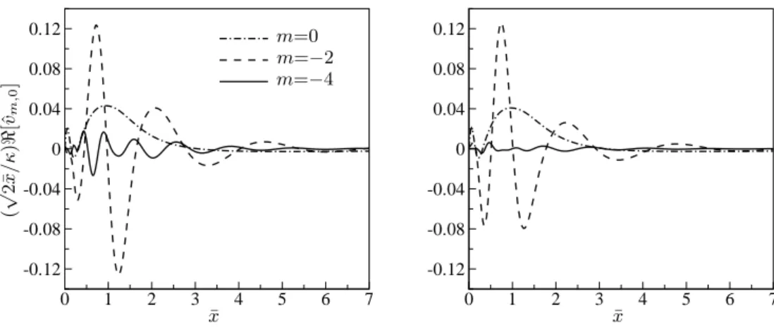
The solution for the irrotational part of the outer flow ¯q0(¯x,y,¯ ¯t) (refer to equation (2.22)) is studied in this section. The streamwise and wall-normal velocity components, ¯
u0(¯x,y,¯ ¯t) and ¯v0(¯x,y,¯ ¯t), are calculated for two different flow regimes: a subsonic case with {M∞, Rλ, rt, κ}={0.69,600,3.6,1.3}and a supersonic case with{M∞, Rλ, rt, κ}={3,1000,
3.6,1.12}.