Dissipation measurements using temperature microstructure from an underwater glider

Contents lists available atScienceDirect

Methods in Oceanography

journal homepage:www.elsevier.com/locate/mio

Full length article

Dissipation measurements using temperature

microstructure from an underwater glider

Algot K. Peterson

∗

, Ilker Fer

Geophysical Institute, University of Bergen, Allégaten 70, 5007 Bergen, Norway

a r t i c l e i n f o

Article history:

Received 16 December 2013 Received in revised form 9 May 2014

Accepted 13 May 2014 Available online 17 June 2014

Keywords: Turbulence Batchelor spectrum Kraichnan spectrum Faroe Bank Channel Glider

Temperature microstructure

a b s t r a c t

Microstructure measurements of temperature and current shear are made using an autonomous underwater glider. The glider is equipped with fast-response thermistors and airfoil shear probes, providing measurements of dissipation rate of temperature vari-ance,χ, and of turbulent kinetic energy,ε, respectively. Further-more, by fitting the temperature gradient variance spectra to a theoretical model, an independent measurement ofεis obtained. Both Batchelor (εB) and Kraichnan (εK) theoretical forms are used. Shear probe measurements are reported elsewhere; here, the thermistor-derivedεBandεKare compared to the shear probe re-sults, demonstrating the possibility of dissipation measurements using gliders equipped with thermistors only. A total of 152 dive and climb profiles are used, collected during a one-week mission in the Faroe Bank Channel, sampling the turbulent dense overflow plume and the ambient water above. Measurement ofεwith ther-mistors using a glider requires careful consideration of data quality. Data are screened for glider flight properties, measurement noise, and the quality of fits to the theoretical models. Resulting dissi-pation rates from the two independent methods compare well for dissipation rates below 2×10−7_{W kg}−1_{. For more energetic}

tur-bulence, thermistors underestimate dissipation rates significantly, caused primarily by increased uncertainty in the time response cor-rection. Batchelor and Kraichnan spectral models give very similar results. Concurrent measurements ofεandχare used to compute the dissipation flux coefficientΓ(or so-called apparent mixing ef-ficiency). A wide range of values is found, with a mode value of

Γ ≈0.14, in agreement with previous studies. Gliders prove to be

∗_{Corresponding author.}

E-mail address:[email protected](A.K. Peterson). http://dx.doi.org/10.1016/j.mio.2014.05.002

2211-1220/©2014 The Authors. Published by Elsevier B.V. This is an open access article under the CC BY-NC-ND license (http:// creativecommons.org/licenses/by-nc-nd/3.0/).

suitable platforms for ocean microstructure measurements, com-plementary to existing methods.

©2014 The Authors. Published by Elsevier B.V. This is an open access article under the CC BY-NC-ND license (http://creativecommons.org/licenses/by-nc-nd/3.0/).

1. Introduction

Direct measurements of turbulent mixing in the ocean require datasets of variables such as small-scale temperature or current shear sampled at high-frequency. Traditionally, such data are acquired using loosely-tethered profilers, deployed repeatedly off a ship’s side (Lueck et al., 2002). This method provides data with little disturbance from vibrations, and repeated profiles can be made relatively fast. However, dedicated ship time is expensive, and microstructure surveys are sporadic. As an alternative, equipping underwater gliders with turbulence sensors facilitates continuous sampling on a low-vibration platform (Fer et al., 2014).

A glider is an autonomous vehicle that moves by changing its buoyancy, and can receive naviga-tional instructions remotely via satellite. The wings, and to a lesser extent a tail fin, translate vertical motion into horizontal motion. This causes the glider to move through the water column in a verti-cal sawtooth pattern, resulting in quasi-vertiverti-cal profiles. Dedicated ship time is not needed, making gliders a potentially very useful platform for turbulence measurements. Another benefit of gliders as an instrument to sample ocean microstructure is their ability to collect data during extreme at-mospheric forcing. During stormy conditions, conducting profiling from ships is hazardous, and such mixing events are thus rarely sampled.

The first attempt to obtain turbulent dissipation rates from a glider was based on an indirect method utilizing standard sensors of the glider:Beaird et al.(2012) analyzed a large dataset from Seaglider (University of Washington) deployments over three years around the Greenland–Iceland– Scotland ridge, and inferred dissipation rates from finescale vertical velocity and density measure-ments. Their method is based on a scaling of the turbulent kinetic energy (TKE) equation, and relies on a scaling constant that is site specific, and accurate vertical water velocity measurements from a glider flight model. Energy loss at viscous scales is inferred from the larger, energy-containing scales. The results from this method compared very well to a co-located microstructure survey from the Faroe Bank Channel (FBC), with an agreement to within a factor of two, when

ε

varied over several orders of magnitude. The method allowedBeaird et al.(2012) to remotely map turbulent mixing and identify turbulent hot-spots in the region using gliders.

The first test using a Slocum electric glider equipped with turbulence sensors was done byWolk et al.(2009) in an approximately 20 m deep freshwater pond. The glider was equipped with a self-contained microstructure instrument package (MicroRider, Rockland Scientific Int., Canada) with shear probes and thermistors. The vertical speed of the glider was typically 10 cm s−1, corresponding to 40 cm s−1_{along the glider’s path, suitable for shear probe measurements.Wolk et al.(2009) found}

the glider to be a favorable platform for turbulence measurements.

The first detailed measurements in the ocean from a glider equipped with shear probes were re-ported byFer et al.(2014). A deep Slocum electric glider equipped with a MicroRider with two shear probes was deployed in the FBC. Dissipation rate measurements from the glider and a ship-based ver-tical microstructure profiler were analyzed and compared. Vibration levels of the glider were generally small, and did not interfere with measurements of small-scale turbulent quantities. The glider mea-surements were shown to be of high quality, with the exception of the turning depths of the glider, where Taylor’s hypothesis becomes invalid. The shear probes were able to resolve dissipation rates of TKE,

ε

, down to 5

×

10−11W kg−1, comparable to the best tethered free-fall profilers. In the turbulent bottom layer of the FBC, average profiles of

ε

from the glider and the microstructure profiler agreed to within a factor of two, whereas higher in the water column averaged glider-derived values were up to 9 times larger than the ship-based measurements. The discrepancies were attributed to the different sampling scheme (glider’s slanted path), spatial and temporal separation between the instruments,

and the intermittency of turbulence. Gliders were, however, concluded to be a suitable platform for ocean microstructure measurements.

The present study is based on the same experiment reported inFer et al.(2014). In addition to shear probes, the MicroRider was equipped with two fast-response thermistors (FP07), providing an additional set of microstructure data. This allows us to compare two independent methods for turbu-lence measurements from the same platform. The aim of this study is to investigate the usefulness of turbulence gliders in a natural and energetic oceanographic environment (see Section4), and to com-pare the results from two methods, based on velocity shear and temperature microstructure. Special emphasis is given to the glider’s thermistor data, including spectral methods to measure the dissipa-tion rates and quality screening, as the shear probe-derived data are already described in detail byFer et al.(2014). We therefore give a summary of temperature gradient spectral forms in the next section. 2. Temperature gradient spectral forms

Stirring of a thermally stratified fluid creates thermal microfronts through strain (Ruddick et al., 2000). Thermal diffusion prevents the gradients from becoming infinitely sharp. Under the assump-tion of small-scale isotropy, the rate of decrease of thermal variance due to diffusion of heat,

χ

, is given by

χ

=

6

κ

T





∂

T′

∂

z



2



,

(1)

where

∂

T′

_/∂

_{zis the small scale vertical temperature gradient;}

_κ

T

∼

1

.

4

×

10−7m2s−1is the molecular

thermal diffusivity; and the angled brackets indicate averaging over a statistically uniform segment. Dissipation rate of TKE,

ε

, is the rate of loss of TKE per unit mass through viscosity to heat (Thorpe, 2007), and has units of W kg−1_{. In an incompressible, homogeneous and isotropic flow,}

ε

=

15 2

ν





∂

u′

∂

z



2



,

(2)

where

ν

is the kinematic viscosity; and

∂

u′

/∂

zis the small scale shear. When shear probe measure-ments are available,

ε

can be directly obtained by integrating the shear wavenumber spectrum.

For a locally isotropic turbulent patch, a one-dimensional temperature gradient spectrum can be calculated from the small-scale temperature gradient. The area under this spectrum is proportional to

χ

. By fitting the observed temperature gradient spectrum to a theoretical model,

ε

can also be deter-mined. TheBatchelor(1959) model is a widely accepted form of the theoretical spectrum (e.g.,Ruddick et al.,2000;Luketina and Imberger, 2001), but the model ofKraichnan(1968) has also been suggested.

Nash and Moum(2002) found that the latter matched their observations more closely than the Batch-elor form.Sanchez et al.(2011) also found the Kraichnan form to be in better agreement with their limnic measurements, particularly at high wavenumbers. Both models are applied in this study, and are described in the following.

Note that wavenumberskin theoretical expressions are typically given in units of radians per meter, while wavenumbers in observed spectra are presented in units of cycles per meter (1 cpm

=

2

π

radian per meter). Here, we use radian wavenumbers in the equations, but use cyclic wavenumbers in the figures, all denoted withk.

2.1. The Batchelor spectrum

Batchelor(1959) was the first to describe the spectrum of a scalar characterized by a large Prandtl number. The Prandtl number is the ratio of the kinematic viscosity to the thermal diffusivity,Pr

=

ν/κ

T. Water temperature is such a scalar. For the viscous wavenumber range,Batchelor(1959) derived

the following three-dimensional temperature spectrum:

φ

T

(

k

)

= −

χ

ζ

kexp



κ

Tk2

ζ



,

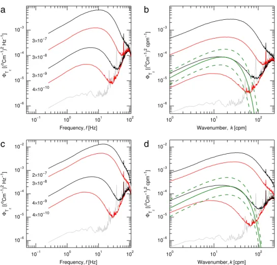
(3)

Fig. 1. Theoretical one-dimensional temperature gradient spectra for different values of (a)ε[W kg−1_{] (withχfixed at}

10−8_{°C s}−1_{) and (b)χ[°C s}−1_{](withεfixed at 10}−8_{W kg}−1_{). Batchelor spectra (green) are shown for four different values}

in each panel, whereas only two examples of the corresponding Kraichnan spectra (dashed red) are shown for clarity. The dotted black curves show the sensitivity to the value ofqB(qB=3, higher maximum at lower wavenumber, andqB=5, lower

maximum at higher wavenumber). In all other Batchelor curves,qB=3.7.

where

ζ

is the average least principal strain rate, acting on scales smaller than the Kolmogorov wavenumberkK

=

(ε/ν

3

)

1/4. The average least principal strain rate for flows at high Reynolds number

is estimated from the Kolmogorov eddies,

ζ

= −

1 qB



ε

ν



1/2

,

(4)

whereqBis a universal constant. The values ofqBreported in the literature vary; the rangeqB

=

3

.

7

±

1

.

5 is typical (Oakey, 1982). In this work,q_B

=

3

.

7 is used, as was done by e.g.,Nash et al.(1999) andPeters et al.(1988).Ruddick et al.(2000) andKocsis et al.(1999) usedqB

=

3

.

4, i.e. 8% smaller

than the value used here. A higher value ofqBresults in a higher maximum at a lower wavenumber, as

shown inFig. 1. A percentage error inqBleads to twice the percentage error in

ε

(Dillon and Caldwell, 1980). By normalizing the wavenumber by the Batchelor wavenumber,

kB

=



ε

νκ

T2



1/4

,

(5)

and the spectral level by

χ(ν/ε)

1/2_k

B−1, the nondimensional form of Eq.(3)becomes

φ

T

(

k

)

kB

χ(ν/ε)

1/2

=

qBkB

k exp

[−

qB

(

kkB

−1

₎

2

_]

_.

₍₆₎

The temperature spectrum can be converted to the temperature gradient spectrum,

φ

Tz, by multiply-ing byk2_{. Note that the spectrum in Eq.(3)is three-dimensional, indicated by the symbol}

_φ

_{. Typically,}

measured temperature spectra are one-dimensional, and the corresponding one-dimensional (indi-cated by the symbolΦ), isotropic form of the temperature gradient spectrum is (Bogucki et al., 2012)

ΦTz

(

k

)

kB

χ(ν/ε)

1/2

=

k 2



qBkB k exp

[−

qB

(

kkB −1

₎

2

_{] +}

_π

1/2_q B3/2

{

erf

[

qB1/2kkB−1

] −

1

}



.

(7)

The temperature gradient spectrum is self-similar, and scales withkB. The curve rises slowly up to the

Batchelor cut-off, and rolls off exponentially for higher wavenumbers. In a log–log plot, changes in

ε

correspond to sliding the graph along a

−

1 slope, while changes in

χ

shifts the spectrum vertically, as illustrated inFig. 1.

The subscriptBwill be used to denote the Batchelor temperature gradient spectra throughout, and to identify

χ

and

ε

derived from fits to the Batchelor form.

2.2. The Kraichnan spectrum

Kraichnan(1968) extendedBatchelor’s work by investigating the effects of fluctuations of the strain rates in time and space, keeping thek−1behavior, but replaced the Gaussian factor in Eq.(3)by a simple exponential. The resulting expression for the one-dimensional isotropic temperature gradient spectrum is

ΦTz

(

k

)

kB

χ(ν/ε)

1/2

=

kkBqKexp

[−

(

6qK

)

1/2_kk

B−1

]

.

(8)

Values of the universal constantqK reported in the literature typically vary between 3.4 and 7.9. We

useqK

=

5

.

26, followingBogucki et al.(2012). Similar to the Batchelor model, increasingqKresults in

a larger spectral maximum at a lower wavenumber. For additional details on the theoretical spectra, the reader is referred to the review byBogucki et al.(2012).

The subscriptK is used throughout to denote the Kraichnan spectrum, and to identify

χ

and

ε

derived from fits to the Kraichnan model. Examples of Batchelor and Kraichnan spectra are shown in

Fig. 1. Batchelor spectra are displayed for varying

ε

(Fig. 1(a)) and

χ

(Fig. 1(b)). For two selected curves in each panel, the corresponding Kraichnan spectra are also shown for comparison. The roll off at high wavenumbers in the Kraichnan model is less steep than in the Batchelor model. The sensitivity toqB

is also shown for the

χ

=

10−9_{°C s}−1_{curve inFig. 1(b), usingq}

B

=

3 andqB

=

5 together with the

defaultqB

=

3

.

7. The sensitivity toqKin the Kraichnan spectrum is similar (not shown).

3. Field experiment

A physical oceanography research cruise to the Faroe Bank Channel (FBC) was conducted on board the research vessel Håkon Mosby, between 26 May and 14 June 2012. Hydrography and current profiles were made using the ship’s CTD (conductivity, temperature, depth) system, equipped with a Sea-Bird Electronics (SBE) 911plus CTD and a pair of lowered acoustic Doppler current profilers (300 kHz RD Instrument Workhorse). Profiles of microstructure were made using a loosely tethered microstructure profiler, VMP2000 (VMP, Rockland Scientific). Additionally, two deep gliders were deployed during the cruise, each equipped with a CTD, and one equipped with turbulence instrumentation. The glider fitted with the turbulence sensors is the focus of this paper. A map of the location is shown inFig. 2, marked with the glider tracks and the VMP stations. For a more complete description of the instrumentation, datasets and the oceanographic context, the reader is referred toFer et al.(2014),Darelius et al.(2013) andUllgren et al.(2014).

The glider used in this study is a Teledyne Webb Research Slocum Electric deep-glider (Jones et al., 2005). The glider is 1.8 m long, with a hull diameter of 22 cm and a wing span of 1 m. It has a mass of about 56 kg, and prior to deployment it is ballasted to be neutrally buoyant in a tank with seawater properties comparable to the deployment site. As a deep glider, it is designed for use down to 1000 m depth. The glider navigates using a rudder on the tail fin, and by moving the central battery pack to shift its center of gravity. Roll is adjusted by rotating the battery; pitch is adjusted by moving the battery back and forth. In the first dive, servo-controlled pitch was allowed to determine optimal battery positions during dives and climbs to maintain approximately

±

25°pitch angles, recommended for nominal endurance. Then the servo was turned off, and the center battery position was manually set to these positions, in order to enable noise-free turbulence measurements.

The glider has an integrated SBE-41 CTD, but for microstructure measurements a Rockland Scientific MicroRider-1000LP (MR, hereafter) turbulence package is used. The package is mounted on top of the glider, and is equipped with two airfoil velocity shear probes, two fast response thermistors (FP07) and high resolution pressure, vibration and tilt sensors. Sensors are located 17 cm ahead and 16 cm off-axis from the glider’s nose, minimizing flow deformation. Temperature, shear and vibration sensors sample at 512 Hz, while the other channels (pitch, roll and pressure) sample at 64 Hz. Equipping a glider with fast-response shear probes and thermistors allows turbulence measurements from two independent methods on the same platform.

Fig. 2. Map of the field work location, including the Faroe Islands and the Faroe Bank Channel. Ship-based microstructure profiler casts are shown as red dots, and the glider track is shown in blue. Two sections, A and C, are highlighted by straight lines. Depth contours are shown every 100 m, the saddle point in the channel is indicated by a black cross. The insert map shows the 500 m isobath and the location relative to Iceland (IC) and Norway (NO).

4. Oceanographic setting

The FBC, with a sill depth of 840 m, is one of the two main passages across the Greenland–Scotland Ridge (GSR) where dense, cold deep water passes from the Nordic Seas to the North Atlantic (Fig. 2). Continuous measurements near the sill covering from 1995 to 2005 showed a total overflow volume flux of 2

.

7

±

0

.

2 Sverdrup (1Sv

=

106_m3_s−1_{), while the volume flux with temperatures lower than}

3°C was 1

.

7

±

0

.

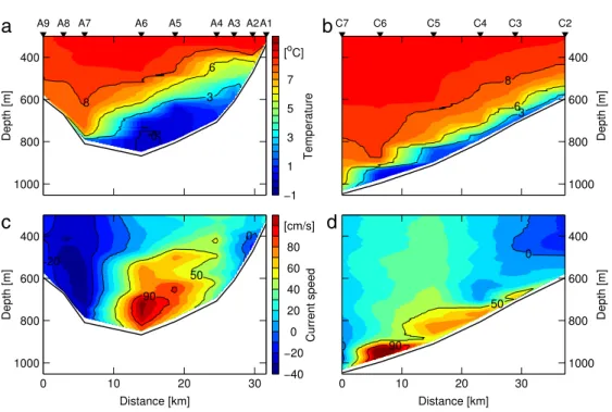
2 Sv (Hansen and Østerhus, 2007). The overflow is associated with oscillations with periods of 3–6 days, with 100–200 m thick domes of cold water flowing along the slope (Darelius et al., 2011). The highly turbulent bottom-attached overflow is approximately 100 m thick, and a turbulent, sheared and stratified interfacial layer of comparable thickness separates the overflow from the ambient water above (Fer et al., 2010). The structure of temperature and along-stream current speed in the overflow is visualized inFig. 3. Two sections based on CTD and LADCP profiles from the present research cruise are displayed, one from the channel, and one from the open slope downstream. Their locations are indicated inFig. 2. Both sections show the cold core of the plume leaning to the right hand slope, with high along-stream current speed, and large vertical gradients in both temperature and current speed.

A cross-stream circulation near the sill, where the flow is constrained by side walls of the channel, was observed byJohnson and Sanford(1992), caused by large frictional stress in the bottom boundary layer. At the interface they found cross-stream velocity in the opposite direction, suggesting a spiral pattern in the flow, causing significant mixing.Seim and Fer(2011) showed that a secondary circulation also existed farther downstream on the Iceland–Faroe slope, driven by the geostrophically-balanced component due to along-channel tilt of isopycnals. The first direct turbulence measurements in the FBC were performed byFer et al.(2010). They found extraordinarily high dissipation rates in the interfacial layer and in the bottom part of the boundary layer, up to 10−5 _{W kg}−1_{. Measurements}

of mixing processes in the overflow are important in order to understand and quantify how the plume properties change as the plume descends the slope, and to determine the depth at which the overflow water becomes neutrally buoyant.

Fig. 3. Two sections of the overflow, color coded for ((a) & (b)) temperature and ((c) & (d)) along-stream current speed. North is to the right in all panels, and positive current speed is directed into the page. The top 300 m are not shown. The sections are located (Section A, (a) & (c)) in the channel and (Section C, (b) & (d)) on the open slope, as marked inFig. 2. Arrowheads and numbered letters at the top mark the profile stations.

5. Data handling 5.1. Glider

The glider data are processed using the software kindly provided by Dr. Gerd Krahmann (GEOMAR, Germany). Raw files are first converted to physical units. Then GPS-fixes and internal navigational calculations are used to calculate a best guess of the glider’s position. Top and bottom turns are identified from pressure records, and the time series are separated into dives and climbs. Unrealistic data are filtered out, and the remainder are interpolated to 1 s time-steps for all sensors.

Salinity is calculated from conductivity, temperature and pressure using the Gibbs SeaWater (GSW) Oceanographic Toolbox (McDougall and Barker, 2011). Potential density anomaly for surface reference pressure (

σ

_θ) is calculated from salinity and temperature, also using GSW.

The direction the glider moves relative to the horizontal, the glide angle,

γ

, is defined as the sum of the glider pitch angle,

θ

, and an ‘angle of attack’ (AOA),

α

, i.e.

γ

=

θ

+

α

. For high quality dissipation rate measurements, glider speed,U, and

α

must be accurately known. A hydrodynamic flight model, described inMerckelbach et al.(2010), is used to obtain the glider speed through waterU, and

α

. The model uses the force balance along the glider’s path. The force balance can be written as

FB

−

Fg

−

ρ

S_wU2

× [

CD0

+

CD1

α

2

_]

2 sin

γ

=

0

,

(9)

which is Eq. 13 ofMerckelbach et al.(2010), corrected for a sign error.FBis the net buoyancy force,

Fg

=

mggis the gravitational force for a glider of massmg,gis acceleration due to gravity,

ρ

is the

in situ density, andS_wis the glider wing surface area. The total parasite and induced drag is deter-mined by the coefficientsCD0andCD1, respectively.CD0is the profile drag coefficient of the glider hull,

CD1 is the sum of the induced drag coefficients of the wings and the hull. The net buoyancy force is

given by

FB

=

g

ρ

{

Vg

[

1

−

chP

+

α

T

(

T

−

T0

)

] +

∆Vbp

}

,

(10)

whereVgis the glider volume,chis the hull compressibility,Pis the water pressure,

α

T is the

ther-mal expansion coefficient,Tis temperature,T0is a reference temperature, and∆Vbpis the buoyancy

change resulting from the buoyancy engine of the glider.

The angle of attack is obtained by numerical iteration of the expression

α

=

CD0

+

CD1

α

2

(

a_w

+

ah

)

tan

(θ

+

α)

,

(11) whereahandaware the lift-slope coefficients for the hull and wings, respectively.

For a deep Slocum glider, the optimized values ofCD1

=

2

.

88,aw

=

3

.

7,ah

=

2

.

4 rad

−1_are

reported inMerckelbach et al.(2010). The variablesT,

ρ

,P,

θ

and∆Vbpare measured by the glider,

andS_w

=

0

.

1 m2_andm

g

∼

56

.

4 kg. The parametersCD0,ch andVg are calibrated for the glider

equipped with the MicroRider by minimizing a cost function relative to the vertical velocity inferred from rate of change of pressure,

w

p, using a non-linear least-squares method. For details on the

op-timization, seeFer et al.(2014). Average values (

±

one standard deviation) areCD0

=

0

.

14

(

±

0

.

02

)

,

ch

=

6

.

1

(

±

0

.

2

)

×

10−10Pa−1, andVg

=

55

(

±

0

.

1

)

×

10−3m−3. In their optimization,Fer et al.(2014)

used the glider mass without the MR mass. The correct value should be approximatelymg

=

62

.

5 kg.

The associated error in the buoyancy force calculation is less than 10%, and is largely compensated for by the optimization of the free parameters. Reprocessing using the correctmg results in

identi-cal average glider speeds, AOA, and dissipation rates within the measurement uncertainty. The drag coefficient here is higher than that reported inMerckelbach et al.(2010), consistent with the approx-imately 30% larger frontal area of a glider equipped with a MicroRider. Once the glider speed,U, and the glide angle are obtained, the vertical speed of the glider is computed as

w

g

=

Usin

(θ

+

α)

.

The average glider along-path speed isU

=

39 cm s−1_andU

₌

_{43 cm s}−1_{, and vertical speed is}

w

g

=

17 cm s−1and

w

g

=

24 cm s−1, for dives and climbs, respectively, see Table 1 ofFer et al.

(2014). The asymmetry in glider speed is not due to the MR, but the manually set central battery positions.

5.2. MicroRider

The time stamp, pressure (P) and temperature (T) records of the MR are corrected against the glider data. Along-path velocity,U, relative to the water, and the vertical velocity,

w

g, are calculated

as described in Section5.1.

Dissipation rates of TKE are calculated using two different methods. One method involves direct measurements of velocity shear. Under the assumption of isotropic turbulence, dissipation rates can be calculated solely from high resolution profiles of velocity shear variance (Eq.(2)), by integrating the wavenumber spectrum. Because of difficulties in resolving scales smaller than the Kolmogorov lengthlK

=

(εν

−3

)

−1/4, the unresolved part of the velocity shear spectrum is accounted for by using

an empirical turbulence spectrum (Nasmyth,1970;Oakey,1982). Additional details on the applica-tion of this method can be found inFer et al.(2014). A subscriptN(for Nasmyth) is used to denote dissipation rates derived from glider shear probes.

The second method involves the measurement of temperature microstructure. Time series from the two thermistors are divided into 12 s half-overlapping segments, corresponding to about 2.4 m vertical segment length. A fast Fourier transform (FFT) length corresponding to 4 s is chosen, and each FFT segment is detrended and Hanning-windowed before calculating the spectra. The segment and FFT length are identical to those used in the processing of the shear probe data. The frequency do-main spectra,Φ

(

f

)

, are converted to along-path wavenumber

(

k

)

domain using Taylor’s frozen tur-bulence hypothesis and the glider speed through water, asΦ

(

k

)

=

UΦ

(

f

)

andk

=

f

/

U. For a typical U

∼

0

.

4 m s−1_{, the FFT length is equivalent to a 1.6 m along-path distance.}

Assuming isotropic turbulence as before, Eq.(1)can be used for glider measurements, using the temperature gradient along the glider’s path,x,

χ

=

6

κ

T





∂

T′

∂

x



2



.

(12)

The glider speed is used to convert time gradient to

∂/∂

x. The fast response thermistor FP07 on the MicroRider has a response time of about 12 ms (1 ms

≡

10−3_{s), due to diffusion and}

attenu-ation of the signal in the boundary layer around the probe. The microstructure spectra are corrected using the dynamic response functionH2

₍

_f

₎

₌

₍

₁

₊

₍

_f

_/

_f

c

)

2

)

−1, wherefc

=

(

2

πτ

U−0.32

)

−1is a

speed-dependent cut-off frequency and

τ

=

12 ms is the thermistor response time (Gregg and Meagher, 1995). The sensitivity of our results to the choice of time constant and the response correction func-tion is discussed in Secfunc-tion7.4.

The temperature profile needs to resolve the Batchelor wavenumber (Eq.(5)), or alternatively a sufficiently – but not completely – resolved gradient spectrum can be fitted to one of the universal forms given byBatchelor(1959) andKraichnan(1968), as described in Section2. We first obtain

χ

by integrating the observedΦTzup to an upper wavenumber,ku, determined as described in Section5.3. The integrated part of the spectrum is significantly above the noise level. We obtained the noise spec-trum,Φn

(

k

)

, by averaging over the quiescent segments of our dataset. We apply a correction to

χ

for the unresolved variance for wavenumbers greater thanku, following the relation in the appendix

ofPeters et al.(1988). We obtain the dissipation rate

ε

from the temperature microstructure using the maximum likelihood estimate (MLE) fit of the observed temperature gradient spectrum to a the-oretical spectrum (Ruddick et al., 2000), constrained by the measured and corrected

χ

. This method allows inclusion of the noise spectrumΦn

(

k

)

in the theoretical spectrumΦth

(

k

)

,

Φth

(

k

)

=

ΦB,K

(

k

)

+

Φn

(

k

),

(13)

whereΦB,K

(

k

)

is the Batchelor or Kraichnan spectrum, Eqs.(7)and(8), respectively. Only the part of

the observed spectrum up tokuis fitted.

An advantage of MLE over least squares, is that for non-Gaussian error distributions, the least squares method is often biased, while the MLE estimates are unbiased (Ruddick et al., 2000). The method also reduces the number of free parameters to adjust, since

χ

is constrained by the integrated temperature gradient spectrum. Only the Batchelor wavenumberkBneeds to be adjusted to fit the

theoretical spectrum, given by Eq.(5), which gives the dissipation rate:

ε

=

k4_B

νκ

_T2

.

(14)

After data quality screening (Section5.3), the results from the two thermistors are checked for consistency, and then averaged.

5.3. Data selection

The MLE fits are made in the portion of each spectrum uncontaminated by noise. The upper wave-number,ku, for integration of a temperature gradient spectrum is chosen as the lowest wavenumber

where the measured spectrum equals 1.5 times the noise spectrum, or at the most, 200 cpm. There is no credibility inΦTz measured by our system at higher wavenumbers. Furthermore, we require at least 5 data points before any fit is attempted.

Ruddick et al.(2000) introduce three rejection criteria for the MLE method, allowing poorly fitted spectra to be identified and discarded automatically. First, the integrated signal-to-noise ratio (SNR) is required to be greater than 1.3, before any fit is attempted. We arbitrarily set SNR

>

1

.

5 as our thresh-old value, i.e., the spectral variance averaged up tokushould be greater than 1.5 times that from the

noise spectrum. Second, the mean absolute deviation (MAD) between the observed and the theoretical spectra,ΦobsandΦth, must be sufficiently small. The deviations are summed up to the wavenumberku,

MAD

≡

1 n ku



ki=k1









Φobs Φth

−



Φobs Φth









.

(15)

FollowingRuddick et al.(2000), a data segment is rejected if MAD is greater than 2

(

2

/

d

)

1/2_{, where}

dis the degrees of freedom of the measured spectrum. This rejection limit is twice the MAD expected from a ‘‘perfect fit’’. A raw periodogram hasd

=

2. For 12 s segments with 4 s FFT length,d

=

6, ignoring the effects of the 50% window overlapping and Hanning windowing.

To ensure that an observed spectrum resolves the sharp roll off of the theoretical spectra, a power-law fit (a straight line in log–log space) is made, which has no roll off. If the theoretical curves do not provide a significantly better fit than the power law, the segment should be rejected (Ruddick et al., 2000). The likelihood ratio (LR), which is the ratio of MLE of the power law fit to the MLE of the theoretical spectrum fit, is calculated as inRuddick et al.(2000). If log₁₀

(

LR

)

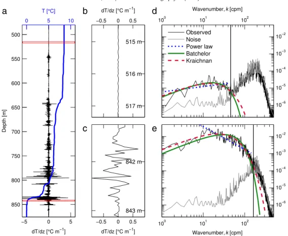
is less than 2, the data segment is rejected, based on the recommendations ofRuddick et al.(2000). This criterion works well for power law fits with a negative slope. However, the slope is positive in the low wavenumber part of the theoretical spectra. When the roll off is located at high wavenumbers, the low wavenumber part of the spectrum increases linearly withk, consistent with the theoretical form. A power law fit will then have a positive slope, and may give a higher likelihood than the theoretical curve, even for a good fit to the theoretical form. We therefore apply the LR criterion only when the power law fit has a negative slope.

Fig. 4shows two examples of observed temperature gradient spectra. The full profiles (below 500 m) of temperature and temperature gradient are shown, together with selected two 12 s seg-ments for which the spectra are presented. Note that this is the segment length used in our data processing, and the spectra are not smoothed, band-averaged or ensemble-averaged over larger seg-ments. The spectra are not exceptional in quality, and are representative of the dataset. The MLE fit of the Batchelor spectrum and Kraichnan spectrum are shown, and the straight lines represent the best power-law fit to each spectrum. Both the quiescent spectrum inFig. 4(d) and the more energetic spectrum inFig. 4(e) show good fits with well-resolved roll offs. The scatter in the spectra are typical for oceanic spectra derived for short segment lengths, and such spectra are not expected to adhere perfectly to the theoretical forms. Kraichnan’s spectrum seems to give a better fit than the Batchelor model for high wavenumbers. This, however, is not true for all spectra.

Taylor’s hypothesis assumes that an eddy does not change significantly as it advects past the measurement point. When the glider speed through water is comparable to the velocity scale of the largest eddies, Taylor’s hypothesis is not valid. The relatively low speed and the slanted path of the glider require careful data selection. FollowingFer et al.(2014), the ratioR

=

U

/

ut, whereUis the

glider’s along-path speed, andutis a turbulent velocity scale, is used to identify the segments that are

suspect to Taylor’s hypothesis. The measured dissipation rates are used to infer a turbulent velocity scale,ut

∼

(ε

l

)

1/3. By substituting the turbulent length scalelby the Ozmidov length scale,

LO

=

(ε/

N3

)

1/2

,

(16)

we obtain

ut

=

(ε/

N

)

1/2

.

(17)

Here, N is the buoyancy frequency, approximated using the observed potential density anomaly profile,

σ

_θ

(

z

)

, N

(

z

)

=



−

g

ρ

0

∂σ

θ

∂

z



1/2

,

(18)

where

ρ

0is a reference density.

An estimate of the noise level for

ε

and

χ

derived from temperature microstructure is calculated. A synthetic spectrum is assigned spectral values 1.55 times our measured noise spectrum, just above our minimum requirement of SNR

>

1

.

5. Then an MLE fit is made to the Batchelor form, giving the lower limits for

ε

=

5

×

10−11W kg−1and

χ

=

1

×

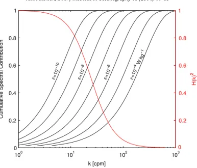
10−11°C s−1. Values lower than this are not resolved by the thermistors, and are excluded from analysis.

The cumulative spectral contribution to

χ

for different values of

ε

is shown inFig. 5. It describes the fraction of

χ

resolved, whenΦTz is integrated up to a wavenumberk. Also shown is the spectral response function using a typical glider speed of 0.4 m s−1_{. The inverse of the response function is the}

Fig. 4. Temperature microstructure from an example profile. Profiles of (a) temperature (blue) and temperature gradientdT/dz (black), and blow up of two 12 s segments ofdT/dzfrom (b) a quiescent and (c) an energetic part of the profile (marked as red rectangles in a). In this presentation the time series are averaged to 4 Hz for clarity. The respective temperature gradient spectra of the two segments ((d) & (e), black) are fitted to a power law (blue dotted line), the Batchelor spectrum (green) and the Kraichnan spectrum (red). The model noise spectrum is indicated (gray). Both spectra show a good fit, and are accepted according to our criteria. In (d), MAD=0.33 andε=1.3×10−9_{W kg}−1_{, and in (e), MAD=0.44, log}

10(LRB)=86.5 and

ε=1.8×10−8_{W kg}−1_{. The log}

10(LR)criterion is not applicable in (d), since the slope of the power law fit is positive (as

explained in the text). The vertical black lines in (d) and (e) indicateku, up to which the fits are made. (For interpretation of the

references to color in this figure legend, the reader is referred to the web version of this article.)

correction needed to compensate for the attenuation in the thermistors power response. For turbulent segments,

ε

is poorly resolved using thermistors. For

ε

=

10−7_{W kg}−1_,

_χ

_{must be corrected by a factor}

of 2 already at approximately 30 cpm, where the response correction on theΦTz is approximately a factor of 4. These corrections are too large, (and particularly the response correction is very uncertain,) and

ε

measurements become inaccurate. We exclude

ε

Band

ε

K greater than 2

×

10−7W kg−1from

the analysis. Note that

ε

Nis properly resolved, and

ε

N

>

2

×

10−7are only excluded when comparing

to

ε

B,K, for consistency.

In summary, average flight properties (U,

w

g,

γ

, AOA), turbulent parameters

ε

and

χ

, andR

=

U

/

ut

are calculated for each 12 s segment. Segments are rejected and excluded from analysis when any of the following conditions are fulfilled (see alsoFer et al., 2014):R

≤

15 for dives andR

≤

20 for climbs, AOA

≥

5,

|

w

_g

|

<

0

.

05 m s−1,

|

w

_g

|

>

0

.

5 m s−1, SNR

<

1

.

5, MAD

>

2

(

2

/

d

)

1/2, log10

(

LR

) <

2,

ε <

5

×

10−11_{W kg}−1_,

_{ε >}

₂

_×

₁₀−7_{W kg}−1_or

_{χ <}

₁

_×

₁₀−11_{°C s}−1_{. After data screening, thermistor}

data was left with approximately 46 000 out of the original 62 000 segments for analysis, distributed as 63% dives and 37% climbs. Shear probe data is reduced from approximately 73 000 to 55 000 data points after data screening, and further down to 51 800 when

ε

N

>

2

×

10−7W kg−1are excluded

Fig. 5. Relative cumulative spectral contribution toχas a function of wavenumber for the Batchelor spectrum withqB=3.7,

andεincreasing from 10−10_{to 10}−4_{W kg}−1_{. For all spectral contribution curves,χ =10}−7_{°C s}−1_{. The spectral response}

function for a glider speed of 0.4 m s−1_{is shown in red. (For interpretation of the references to color in this figure legend, the}

reader is referred to the web version of this article.)

6. Results

6.1. Average spectra

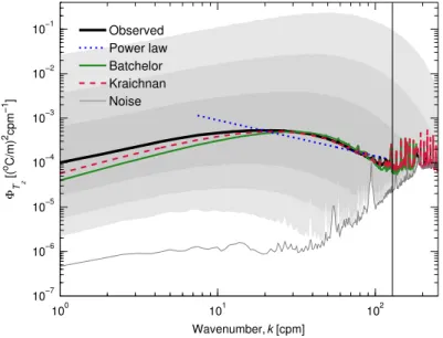
Observed temperature gradient spectra span a wide range of turbulence levels, from the quiescent interior to the highly turbulent plume interfacial and bottom boundary layers. An overview of all spec-tra from segments which passed the quality screening is shown inFig. 6, where gray shading indicates the span of spectral values at selected percentiles. The average spectrum between the 45–55th per-centiles shows a shape similar to the theoretical Batchelor and Kraichnan forms in the dissipation sub-range, between 5 and 100 cpm. We restricted the example average spectrum to a narrow percentile range because averaging over a large range of

ε

and

χ

will distort the spectral shape (i.e., individ-ual spectra are not sampled from a homogeneous turbulent patch). For the low wavenumbers, in the viscous-convective subrange, the observed spectrum has a gentler slope than the theoretical forms. The dissipation rates obtained from the fits are

ε

B

=

1

.

4

×

10−8W kg−1and

ε

K

=

1

.

3

×

10−8W kg−1,

and

χ

=

2

.

6

×

10−8°C s−1.

The range and quality of the observed temperature gradient spectra are again demonstrated in

Fig. 7, where spectra are averaged in decadal bins of

χ

and

ε

in the range 10−6_–10−10_{for both}

_ε

(W kg−1) and

χ

(°C s−1). Thousands of spectra are averaged, seeTable 1for details. The averaged spectra are displayed with respect to both frequency and wavenumber. Fits of the Batchelor form to selected averaged spectra are also shown. In a given

χ

or

ε

bin, the corresponding parameter spans one order of magnitude (by definition) and the other parameter can vary even more. The average spectrum is thus not representative of a homogeneous patch with given

ε

and

χ

, and will differ from the theoretical form. The expected variability in the spectral form for each bin can be estimated by the Batchelor spectrum calculated using the observed variability in

ε

and

χ

. The dashed envelope in

Figs. 7(b) and7(d) shows the Batchelor spectrum for

±

0.5 standard deviation variability. The variable glider speed also distorts the spectral shape, but this is found to be negligible (variability in a given bin is less than 5%).

All presented average or individual spectra of temperature gradient closely follow the Batchelor or Kraichnan forms in the diffusive subrange where the spectra roll off. These are the scales that contain

Fig. 6. Overview of the temperature gradient spectra from the 46 000 segments that are of good data quality. The gradually darker gray shadings are defined by the 2nd/98th, 10th/90th and 25th/75th percentile values at each wavenumber, respectively. A mean spectrum of all spectral values within 5% of the median is shown in black together with the MLE-fitted Batchelor spectrum (green), Kraichnan spectrum (dashed red) and a power law fit (dotted blue). The noise spectrum is shown by the gray line. The vertical black line indicatesku, the wavenumber up to which the fits to the average spectrum are made. The values

obtained from the MLE fit areεB=1.4×10−8W kg−1,εK =1.3×10−8W kg−1andχ=2.6×10−8°C s−1.

Table 1

Number of segments with goodΦTz-spectra in decadal bins ofεandχ, used for calculating bin averaged spectra inFig. 7. The bin range is in units of W kg−1_{forεand°C s}−1_forχ.

Bin range ε-binned χ-binned [10−10₁₀−9_{] 6 587 4 635} [10−9₁₀−8_{] 16 374 12 007} [10−8₁₀−7_{] 19 516 13 708} [10−7₁₀−6_{] 2 941 9 513}

most of the gradient variance. At the lower wavenumbers in the viscous-convective subrange with k+1 _{slope, spectral amplitudes are up to a factor of 2 greater than the theoretical shapes. Similar}

deviations are reported extensively in the literature (Dillon and Caldwell, 1980;Nash and Moum, 2002;Oakey,1982;Sanchez et al.,2011), especially for small Cox numbers (Cx

= ⟨

dT′

/

dz

⟩

2

/

⟨

dT

/

dz

⟩

2).

Typically, the deviations are attributed to remnant background vertical temperature structure (Dillon and Caldwell, 1980;Nash and Moum, 2002), or, inverse cascade of a fraction of the spectral peak to lower wavenumbers (Nash and Moum, 2002).

6.2. Shear probe and thermistor comparison 6.2.1. Average profiles

In order to present and quantify the performance of the thermistors in measuring

ε

, a comparison to shear probes is first attempted in the average sense. This also ensures that sufficient sampling and averaging is made over the 3–6 day period oscillation which dominates the variability at the site (see Section4). Survey averages are made from the glider thermistor data (Batchelor,

ε

B, and

Kraichnan,

ε

K, MLE fits), and shear probe data (Nasmyth,

ε

N) from the glider. To determine the vertical

a

b

c

d

Fig. 7. Temperature gradient spectra, averaged in decadal bins with respect to ((a) & (b))χand ((c) & (d))εbetween 10−10_and

10−6_{. Noise spectra are shown in gray. Panels (a) and (c) show frequency spectra, while (b) and (d) show wavenumber spectra.}

The average values ofχ[_°C s−1_{]andε[W kg}−1_{] in each bin are given in panels (a) and (c), respectively. For clarity, a Batchelor fit}

(green) is shown for only one mean spectrum in each of panels (b) and (d). The dashed Batchelor spectra envelop 0.5 standard deviation variability inεandχin the chosen decadal bin. (For interpretation of the references to color in this figure legend, the reader is referred to the web version of this article.)

et al.(1993). The test determines, within a 5% significance level, whether consecutive values are correlated or not. We perform the test for glider-derived dissipation rates of TKE, from both shear and temperature gradient spectra. Only data from depths between 100 m and 250 m are used, to ensure uniform stratification. For bin sizes of 1–2 m, over 50% of the profiles are rejected as correlated, but with increasing bin size, the rejection ratio reduces to approximately 10% for 10 m bins. When the bin size is further increased to 15 m, the rejection percentage is below the 5% significance level. Thus 15 m bin averages are treated as uncorrelated, and the profiles are averaged in 15 m vertical bins. The test shows similar results for both temperature- and shear-derived

ε

.

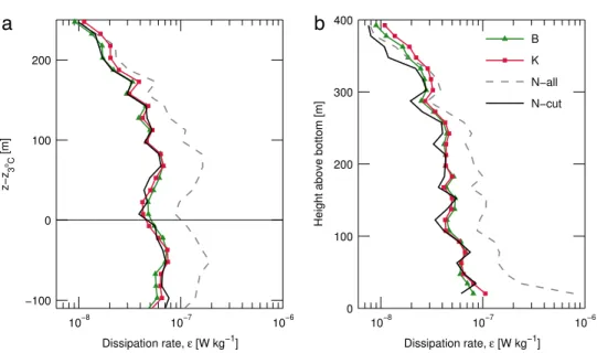
Survey-averaged

ε

profiles are calculated relative to the 3°C-isotherm depth and as height above bottom (HAB), and are shown inFig. 8. The 3°C isotherm is a useful identifier of the interface between the dense plume and the interfacial layer above. Two versions of the shear-derived dissipation rate (

ε

N) profiles are shown; one profile excludes

ε

N

>

2

×

10−7W kg−1to be consistent for

compari-son with thermistor data, the other profile includes all quality screened

ε

Nin averaging. The latter is

Fig. 8. Survey-averaged profiles of dissipation rates of TKE from the glider using shear (Nasmyth; values ofε >2×10−7

excluded for comparison, in black, and the complete version for reference, dashed gray) and temperature microstructure; Batchelor fit (green) and Kraichnan fit (red). Data are vertically averaged in 15 m bins with respect to (a) the 3°C isotherm, indicative of the dense plume interface, and (b) height above bottom (HAB). (For interpretation of the references to color in this figure legend, the reader is referred to the web version of this article.)

boundary layer, and in the turbulent interface. When

ε

N

>

2

×

10−7W kg−1are excluded from

aver-aging, the agreement between the methods is very good. For low dissipation rates, above 300 m HAB, the two versions of

ε

Nagree closely. Closer to the bottom, the offset between the two shear profiles

increases, as expected because of the increasing dissipation rates. As a result of the thermistors’ in-ability to resolve the most energetic turbulence, the mean profiles of

ε

B,Kshow only a slight increase

in dissipation rates towards the bottom.

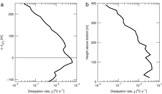
A survey-averaged profile of

χ

is shown inFig. 9. (Profiles for

χ

are identical for Batchelor and Kraichnan, because

χ

is obtained by integrating the temperature gradient spectrum to constrain the theoretical spectra.) There is a gradual increase in

χ

towards the bottom. The survey average relative to the 3°C isotherm reveals a peak in

χ

at 3°C, about one order of magnitude higher than just 100 m above or below. The 3°C isotherm is in the stratified interfacial layer (Fig. 4), where the background temperature gradient is large and the current shear is strong. The increase in

χ

in this layer is consistent with substantial temperature variance production by the background gradient and local destruction. The decrease in

χ

below the interface depth is consistent with a weaker temperature gradient compared to the interface.

Profiles of

ε

and

χ

are similar in vertical structure, and both show a gradual increase with depth towards the turbulent plume. There are differences in the turbulent interfacial layer and the bottom layer, however. A pronounced peak is observed in

χ

at the interface in contrast to

ε

that is relatively constant within

±

100 m of the interface depth. Below this level,

ε

remains high, while

χ

decreases towards the bottom with respect to the interface depth. In the bottom 100 m,

χ

remains fairly uniform, whereas

ε

N increases. Current shear remains strong below the interface, while the temperature

variance is reduced due to the weaker background temperature gradient in the quasi well-mixed bottom layers. In the limiting case of very well-mixed homogeneous bottom layer, the stratified temperature variance model breaks down. Survey-averaged profiles of temperature and velocity inferred from CTD/LADCP stations show that the maximum vertical temperature gradient is located at the interface whereas the velocity shear maximum is approximately 25 m above (not shown). The mean velocity profile has a maximum at approximately 20 m below the interface, corresponding to a minimum in shear, hence local shear production of TKE. This is likely the main reason for the difference

Fig. 9. Survey-averaged profiles ofχ. Data are averaged vertically in 15 m bins with respect to (a) the 3°C isotherm, indicative of the dense plume interface, and (b) height above bottom (HAB).

between the

ε

and

χ

profiles at the interface, however, buoyancy effects and anisotropy can also be important.

6.2.2. Probability distributions

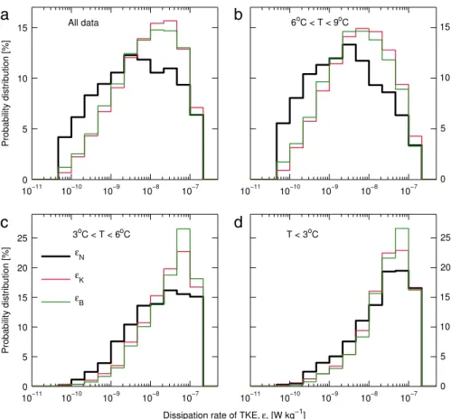
Probability distributions of measured

ε

are shown inFig. 10, for all data, as well as for three temper-ature range subsets, corresponding to the dense overflow (T

<

3°C), the interfacial layer (3°C

<

T

<

6°C) and the ambient layer (6°C

<

T

<

9°C). For the sake of comparison,

ε

N

>

2

×

10−7 W kg−1

are excluded to be consistent with

ε

B,K. Compared to

ε

N, measured by the shear probes,

ε

Band

ε

K,

measured by the thermistors, show a narrower distribution with relatively more frequently observed intermediate dissipation rates, and less frequent low dissipation rates. The 3–6°C range is where both

ε

Band

ε

K deviate the most from

ε

N, in the high dissipation tail of the distribution. The distributions

of

ε

Band

ε

Kare very similar, except that, although in the same

ε

band, the peak values forT

<

6°C

have approximately 5% more contribution in

ε

B.

6.2.3. Individual profiles

The survey-averaged profiles of

ε

Nand

ε

Bcompare very well (Fig. 8). Since they are sampled from

the same platform, individual profiles can be contrasted. Two example profiles, one dive and one climb, are shown inFig. 11. The profiles of

ε

and

χ

are averaged in 15 m bins. Profiles of

ε

Bfollow

ε

Nclosely, indicating a very good agreement between the two methods. (Profiles from the Kraichnan

model,

ε

K, similarly agree with the shear-probe results,

ε

N, not shown for clarity.) This is generally

the case for all individual profiles. A tendency to underestimation of

ε

Bis seen when

ε

Napproaches

∼

10−7 _{W kg}−1_{. Close to the bottom, many data segments are missing (see the bottom 100 m in} Figs. 11(e)–(h)), mainly because

ε >

2

×

10−7_{W kg}−1_{. In the upper part of the water column the}

glider flight properties (U,

w

gand AOA,Figs. 11(c), (d), (g) and (h)) are relatively smooth. As the glider

crosses the plume interface there is substantial variance in glider speed and AOA which persists in the turbulent, highly-sheared bottom boundary layer.

To further investigate similarities and differences between individual

ε

N and

ε

B, profiles, a

scatterplot of

ε

Nand

ε

Bis shown inFig. 12, color coded for temperature. Both variables are averaged

vertically in 15 m bins. Data points are excluded when there are less than 5 data points in a given bin, or when the mean temperature gradient in the bin is positive (i.e., unstable over the whole segment).

a

b

c

d

Fig. 10. Probability distribution functions ofε, obtained from the Batchelor (εB, green), Kraichnan (εK, red) and Nasmyth (εN,

black) forms. In (a), all data (ε <2×10−7_{W kg}−1_{) are included, while the rest are conditionally sampled for temperature}

classes (b) 6°C<T<9°C, (c) 3°C<T<6°C and (d)T<3°C. (For interpretation of the references to color in this figure legend, the reader is referred to the web version of this article.)

85% of the data points agree to within a factor of

(

22

+

22

)

1/2

=

2

.

8, corresponding to propagation of a factor of two error in both variables. Dissipation rates

ε >

2

×

10−7_{W kg}−1_and

_{ε <}

₅

_×

₁₀−11_{W kg}−1

are removed in the data screening. Still, a tendency towards underestimation of

ε

Bcan be observed

for large

ε

N, which is also associated with cold water. However, this is often within the typical (factor

of two) uncertainty of the data. 6.3. Dissipation flux coefficient

The dissipation flux coefficient,Γ, is commonly used to infer eddy diffusivity, and hence turbulent buoyancy or heat fluxes, from measurements of

ε

. When both

ε

and

χ

are measured simultaneously, an estimate ofΓcan be made from

Γ

=

χ

N

2

2

ε

⟨

Tz

⟩

2

,

(19) (Gargett and Moum, 1995).Ruddick et al. (1997) call this quantity the dissipation coefficient, or apparent mixing efficiency. The flux coefficient is closely related to the mixing efficiency,Rf

=

Γ

/

(

1

+

Γ

)

. From the 15 m vertically averaged dataset, approximately 1100 values ofΓ are calculated. Here we use

ε

N which is better resolved than

ε

B,K. (It is here not recommended to inferΓ using

c

d

e

f

g

h

a

b

Fig. 11. Two example pseudo-vertical glider profiles, where panels (a) and (e) show the dissipation rate of TKE inferred from shear (εN, black) and temperature (Batchelor fit,εB, green), panels (b) and (f) show the dissipation rate of thermal variance,χB,

panels (c) and (g) show vertical glider velocity (wg, red) and temperature (T, black), and panels (d) and (h) show along-path

glider velocity (U, red) and AOA (black). Dissipation rates are averaged in 15-m vertical bins. The upper and lower panels are from one arbitrary deep dive and climb, respectively. (For interpretation of the references to color in this figure legend, the reader is referred to the web version of this article.)

orders of magnitude, but only 9% of the data points lie above 1. The distribution shows a single maximum, and using a bin width of ₃₀1, the mode value is 0.14. The geometric mean and the median are both 0.33.

The mixing efficiency has previously been shown to depend on the turbulence activity index, IA

=

ε/ν

N2, which is a commonly used parameter for quantification of turbulence intensity (Shih et al., 2005). We calculated the maximum likelihood estimate ofΓ in bins ofIAin the range from 100

to 105_{. As seen inFig. 14, betweenI}

A

=

100 andIA

∼

2

×

104, there is a steady decrease inΓ for

increasing turbulence intensity. Error bars indicate the 95% upper and lower limits of the estimates. The trend inΓis thus statistically significant. The large error bars at the high and low ends ofIAreflect

that fewer values are available for the calculations in those bins. The measurement uncertainty of an individualΓestimate can be larger than the statistical uncertainties as a result of the typical a factor of two uncertainty in dissipation measurements. The dissipation flux coefficient values, however, are most meaningful in the average sense, averaged over life span of many turbulent eddies. Averaging reduces the errors associated with the dissipation measurements. Although not formally calculated, the accuracy of bin-averagedΓis estimated to be comparable to the error bars inFig. 14.

Fig. 12. Comparison of dissipation rates of TKE derived from the Batchelor fits (εB) and the shear probes (Nasmyth,εN). Markers

are color coded for temperature. The solid line represents a one-to-one agreement, the dashed and dotted lines mark deviations of factors 2.8 and 10, respectively.

a

b

Fig. 13. Probability distribution of the dissipation flux coefficientΓ, shown in (a) 30 logarithmically-spaced bins between 10−2

and 101_{, and (b) in 30 linearly-spaced bins between 0 and 1. The mode value is 0.14 (using a bin width of} 1

30), the median and

Fig. 14. Dissipation flux coefficient,Γ, versus the turbulence activity indexIA =ε/νN2, calculated as maximum likelihood

estimates in bins ofIA. Error bars represent the upper and lower 95% limits of each bin.

7. Discussion

7.1. Glider as a platform for turbulence measurements

Ocean microstructure measurements require sufficient sampling to increase the statistical reliabil-ity, and also to average over the inherent intermittency. Furthermore, the methods require a vibration free platform, and specific ranges of speed with which the sensors should move through the water, away from unnatural disturbances and sources of artificial turbulence. The gliders, although not de-signed for this purpose, are promising platforms that can return high quality and cost-efficient ocean microstructure data.

Caution must be exercised, however, in processing and interpreting the data from gliders. Careful data screening is crucial because there may be portions of the slant profiles which violate the assump-tions behind the methods by which the dissipation rates are obtained. Different datasets and environ-ments may call for different criteria and computations for rejection of suspect data. Our dataset is from a challenging oceanographic environment, where the glider experiences navigation difficulties, and it cannot penetrate across the sheared, stratified overflow-ambient interface smoothly and rapidly. Furthermore, the angle of attack and speed of the glider through water must be determined as accu-rately as possible, necessitating an applicable flight model with site- and glider-specific coefficients. Overall, after data screening, we are left with 75% (shear probes) and 74% (thermistors) of the original dataset. Nevertheless, the amount of data and the quality of the measurements are overwhelming, and can lead to a step increase in our present sampling capabilities and understanding of the ocean mixing processes.

7.2. Dissipation measurements using thermistors

In this study, we utilized two completely independent methods using measurements from shear probes and thermistors to sample the dissipation rate of TKE,

ε

Nand

ε

B(and

ε

K), respectively. While

the Slocum glider allows easy integration of the MR, gliders fitted with only thermistors are of interest. For this purpose we conducted a detailed comparison of

ε

measured by the two different methods. The agreement between the two methods lends confidence on the skill of microstructure measurements from gliders, in general, and for the use of thermistors in a limited range of dissipation rates, in par-ticular. A comparison of

ε

Nand

ε

Bshows that in segments that are above the noise level, but not very

energetic, the two methods agree to within a measurement uncertainty of a factor of two, for individ-ual segments of 15 m vertical extent. The agreement improves with further averaging. For energetic segments, when dissipation rates exceed

ε

=

2

×

10−7_{W kg}−1_{, the thermistor’s time response}

cor-rection becomes uncertain, and the temperature gradient spectra are not sufficiently resolved. The turbulent bottom boundary layer (BBL) is one such region where the discrepancy is substantial. Ex-cluding all segments with

ε >

2

×

10−7 _{W kg}−1_{, from both}

_ε

N and

ε

B,K, allows a comparison of

similarly subsampled datasets. The comparison of the subsampled data shows very good agreement, with discrepancy less than 2% when averaged with respect to the 3°C isotherm depth, or 15% with respect to HAB. Although this agreement demonstrates the capability of thermistors to measure

ε

, the discrepancy from the actual (not subsampled)

ε

profile can be large for energetic turbulence. For

ε

N

∼

10−7W kg−1,

ε

Bunderestimates by a factor of 2, and for

ε

N

∼

10−6W kg−1, the discrepancy

reaches one order of magnitude.

The MLE fits of Batchelor and Kraichnan models to observations were generally very good, as demonstrated for individual segments inFig. 4. In a comparison of the Batchelor and the Kraichnan spectral fits,Sanchez et al.(2011) found that the Kraichnan form gave a better fit to their data, and that the Batchelor fit underestimated at high wavenumbers. In the energetic segment shown inFig. 4, the Kraichnan form is in slightly better agreement with observations than the Batchelor form. The Kraich-nan model does not always give the best fit, however, and in the survey-averaged profiles (Fig. 8), these differences are not apparent. High wavenumbers dominate in the turbulent bottom boundary layer, and based on the findings ofSanchez et al.(2011),

ε

Bcould be expected to underestimate compared to

ε

Kin the survey-averaged profiles. This is, however, not observed. In our dataset the choice of spectral

fit to the temperature variance spectra does not appear to influence the final results significantly. The mean profiles of

ε

Band

ε

Kare identical within the measurement uncertainty.

Oakey(1982) reported

ε

from both thermistors and shear probes, using the microstructure profiler OCTUPROBE II. He concluded that the two measurement techniques agree to within a factor of 2 on average, similar to our results. It should be noted that his analysis is limited to 25 segments of mi-crostructure measurements. The dataset does not include

ε >

5

×

10−7W kg−1, consistent with our approach (to exclude unresolved

ε

). Our results can also be compared toKocsis et al.(1999), who re-ported measurements of

ε

from current shear and temperature microstructure in the surface layer of a lake. Similar to our observations (Fig. 12),Kocsis et al.(1999) found agreement between the two meth-ods to be within a factor of 2 for the bulk of the measurements, but under certain circumstances, dis-crepancies up to a factor of 10 were observed. They attributed these features to the spatial resolution of the temperature microstructure data, and the noise levels of the shear probes. Note that the measure-ments byKocsis et al.(1999) were made using two independent ideal instrumentations and sampling schemes required by the two different methods (shear and temperature microstructure measure-ments). Their results show that

ε

is overestimated by the thermistors for low turbulence, and under-estimated for energetic turbulence, similar to what is observed inFig. 10. Considering their dataset and results as state-of-the-art, we conclude that the glider measurements are of comparable quality. As the turbulent activity indexIAdecreases, buoyancy effects become increasingly more important

and velocity fluctuations become anisotropic. In such conditions, typical in theT

>

3_°C range (see Fig. 13(b) ofFer et al.(2014)), we observe a substantial bias in the ratio

ε

B

/ε

N. When averaged over

ensembles withIA

<

100 (where anisotropy is expected),

ε

B

/ε

N

=

2

.

4, whereas in the range 100

<

IA

<

104,

ε

B

/ε

N

∼

1. This leads to a skewness in the probability distribution as seen inFig. 10. This may

be attributed to our use of constantqB. Several studies leftqBas a free parameter and determined it

individually for each patch (see e.g.Nash and Moum, 2002).Gargett(1985) reported a large difference inqBbetween isotropic (qB

=

12) and anisotropic (qB

=

4) temperature gradient spectra. The quality

of dissipation measurements from thermistors and the comparison with

ε

Ncan perhaps be improved

ifqBis determined for each individual spectrum. This, however, is not tested in the present study.

7.3. Flux coefficient

Smyth et al.(2001) studied the time evolution of the flux coefficient using numerical simulations, which showed thatΓ varied by more than one order of magnitude over the lifetime of a turbulent overturn. With time, it approached the asymptotic value of 0.2. Our measurements show a wide range