ground-based sensor synergy at
Ny-Ålesund
inaugural-dissertation
zur
Erlangung des Doktorgrades
der Mathematisch-Naturwissenschaftlichen Fakultät
der Universität zu Köln
vorgelegt von
Tatiana Nomokonova
aus
Krasnokamensk
Russland
Köln
2020
Prof. Dr. Roel A.J. Neggers
Tag der letzten mündlichen Prüfung: 15 May 2020
Contemporary climate models show that clouds are one of the key components in the climate of the Arctic region experiencing rapid surface warming. Modeling of the cloud impact on the Arctic amplification is still uncertain not only because cloud life cycle is defined by large number of processes, but also because the clouds are closely related to other components of the Arctic climate, such as atmospheric water vapor, ocean, sea ice, and long-range air transport. In order to better understand the role of clouds in the Arctic, in June 2016 the French-German Arctic research station situated in Ny-Ålesund, Norway was complemented with a W-band cloud radar within the Transregional Collaborative Research Center (TRR 172) "Arctic Amplification: Climate Relevant Atmospheric and Surface Processes, and Feedback Mechanisms (AC)3". This observation site became one of a few Arctic sites capable
of state-of-the-art cloud profiling with high temporal and spatial resolution. This thesis summarizes the cloud macro and microphysical properties of clouds based on the first two and a half years of cloud measurements at Ny-Ålesund. The total occurrence of clouds was found to be∼81%. The most predominant type of clouds is multi-layer clouds with the frequency of occurrence of 44.8%. Single-layer clouds occur 36%of the time. The most common type of single-layer clouds is mixed-phase with a frequency of occurrence of 20.6%. The total occurrences of single-layer ice and liquid clouds are 9% and 6.4%, respectively. A comparison of cloud occurrence at Ny-Ålesund with a numerical weather prediction model revealed an overestimation in the occurrence of single layer ice clouds and underestimation of the occurrence of mixed-phase clouds.
The cloud properties were further related to occurrence of anomalous atmospheric conditions often caused by transport of relatively warm and moist air from the North Atlantic and circulation of dry and cold air in the Arctic region. Dry anomalies are related to about 30% less cloud occurrence with respect to normal conditions. In contrast, during moist conditions the cloud occurrence typically reaches 90–99%. Excess and shortage in water vapor typically increases and decreases the amount of condensed water in cloud, respectively. The changes in cloud properties during moist and dry anomalies in turn affect the surface cloud radiative effect (CRE). In winter, spring, and autumn the net surface CRE is dominated by the longwave (LW) CRE and, therefore, during these seasons dry and moist conditions are related to lower and higher cloud related surface warming in Ny-Ålesund, respectively. In summer, shortwave CRE becomes dominant and moist conditions cause stronger surface cooling relative to normal cases, while dry conditions tend to reduce the cloud related surface cooling.
Moist anomalies show significant positive trends varying for different seasons from 2.8 to 6.4% decade−1. In contrast, the occurrence of dry anomalies has been
clining at rates from −12.9 to−4% decade−1. A novel technique for the estimation of LW CRE developed within this study shows that the long-term trends in the thermodynamic conditions at Ny-Ålesund are related to significant positive trends in longwave CRE of 3.4 and 2.2 W m−2 decade−1 in winter and autumn, respec-tively. In summer, a negative trend of −1.8 W m−2 decade−1 was found, while no significant trends were found for the spring season. The database with cloud profiles obtained within this work can be used for an evaluation of numerical weather pre-diction models, while radiative cloud properties estimated from reanalysis models can be evaluated with long-term LW CRE retrieved with the developed method.
Aktuelle Klimamodelle wie auch Beobachtungen zeigen, dass sich die Oberfläche der Arktis schneller erwärmt als die globals Mitteltemperature, diesen Effect bezeichnet man als "Arctic Amplicfication". Der Einfluss von Wolken auf "Arctic Amplifi-cation" ist immer noch unsicher. Dies liegt nicht nur an den vielen verschiede-nen Prozesse welche zum Teil noch nicht vollständig verstanden sind, sonder auch an anderen Komponenten des Klimasystems wie Wasserdampfgehalt der Luft, In-teraktion von Ozean oder Meereis mit der Atmosphäre, und dem Luftmassenfer-ntransport in die Arktis. Um die Rolle arktischer Wolken besser zu verstehen, wurde im Rahmen des überregionalen Forschungsverbundes (TRR 172) "Arctic Am-plification: Climate Relevant Atmospheric and Surface Processes, and Feedback Mechanisms (AC)3" im Juni 2016 die deutsch-französische Forschungsstation
AW-IPEV um ein W-Band-Radar ergänzt. Somit ist diese Beobachtungsstation eine der wenigen in der Arktis, die "state-of-the-art" Wolkenbeaobachtungen mit ho-her zeitlicho-her und räumlicho-her Auflösung ermöglichen. Diese Arbeit fasst die makro-und mikrophysikalischen Eigenschaften der Wolken in den Messungen der ersten zweieinhalb Jahre in Ny-Ålesund, Spitzbergen, zusammen. Dabei war es über 81% der Beobachtungsyeitraumes bewölkt, 44.8% der Zeit dominierten Mehrschichten-wolken beobachtet, 36% der Zeit einschichtige Wolken. Unter den EinschichtMehrschichten-wolken traten Mischphasenwolken mit 20.6% am häufigsten auf, Eiswolken mit 9% und Wasserwolken mit 6.4%. Ein Vergleich der Auftretenshäufigkeit der verschiedenen einschichtigen Wolkenarten zwischen nummerischen Wettervorhersage und Beobach-tungen in Ny-Ålesund zeigte, dass das Vorkommen von einschichtigen Eiswolken im Model überschätzt und das Auftreten von Mischphasenwolken unterschätzt wird. Weiter wurden die Wolkeneigenschaften mit dem Auftreten von ungewöhnlichen Wetterlagen detalieiert untersucht, insbesondere dem Anomalien des integrierten Wasserdampfgehalt. Diese Anomalien werde durch den Luftmassenferntransport in die Arktis herforgerufen. Eine feuche Anomalie wird durch den Transport von war-men und feuchte Luftmassen, die mit Anströmungen vom Nordatlantik einherge-hen, erzeugt, eine trockene Anomalie wird durch die arktische Zirkulationen her-vorgerufen. Bei einer feuchten Anomalie kam es zu einer Wolkenauftretenswahrschein-lichkeit von 90-99% bei den trockenen Anomalien wurde 30% weniger Wolkenbe-deckung beobachtet, als unter normalen Bedinungen. Die Menge von verfügbarem Wasserdampf beeinflusst die Menge an kondensiertem Wasser in der Wolke, was zu Veränderungen der microphysikalischen Wolkeneigenschaften führt und somit zu einer eine Veränderung des "Cloud radiative effect" (CRE) am Boden. Im Winter, Frühling und Herbst ist der netto CRE in Ny-Ålesund vor allem von der lang-welligen Strahlung abhängig und bringen so eine stärkere Oberflächenerwärnung während negativer Feuchteanomalien mit sich. Im Sommer hat die kurzwellige
Strahlung einen größeren Einfluss. Wolken, die während positiver Feuchteanoma-lien auftreten haben einen negativen CRE und während negativer FeuchteanomaFeuchteanoma-lien verringert sich die Kühlung, die mit den Wolken in dieser Jahreszeit einhergeht. Pos-itive Feuchteanomalien zeigen je nach Jahreszeit posPos-itive Trends zwischen 2,8 und 6,4% pro Dekade. Im Gegensatz dazu nimmt die Auftretenshäufigkeit der negativen Feuchteanomalien mit -12,9 bis -4% ab.
In dieser Arbeit wurde eine neue Methode zur Abschätzung des langwellingen CRE entwickelt. Es konnte gezeigt werden, dass der langfristige Trends der thermody-namischen Bedingungen in Ny-Ålesund mit dem signifikanten positiven Trends des langwellingen CRE im Winter (3,4 W/m−2 pro Dekade) und Herbst (2,2 W/m−2 pro Dekade) in Verbindung steht. Im Sommer wurde eine Abnahme des langwellige CRE um 1,8 W/m−2 pro Dekade ermittelt wo hingegen sich für den Früling kein sig-nifikanter Trend zeigte. Dieser Datensatz, mit den hier abgeleiteten Wolkenprofilen, kann auch zukünftig genutzt werden um numerische Wettermodelle zu evaluieren. Ebenfalls können die Strahlungseigenschaften aus der in dieser Arbeit entwickel-ten Methode benutzt werde um Reanalysedaentwickel-ten abgeleiteentwickel-ten langwelligen CRE zu verglichen.
1 Introduction 1
1.1 Role of clouds in the radiation budget . . . 3
1.2 Role of clouds in the Arctic warming . . . 5
1.3 Studies on feedback processes in the Svalbard region . . . 7
1.4 Coupling of cloud and environmental properties to SW and LW CRE 9 1.5 Estimation of CRE from observations . . . 13
1.6 Observations of cloud properties in the Arctic . . . 15
1.7 Focus and scientific questions of the thesis . . . 18
2 Instrumentation and data products 21 2.1 Cloud radar . . . 21
2.2 Microwave radiometer HATPRO . . . 23
2.3 Ceilometer . . . 26
2.4 Radiosondes . . . 27
2.5 Baseline surface radiation network BSRN . . . 27
2.6 Cloudnet data products . . . 29
2.7 Cloud microphysical dataset . . . 34
2.8 Model data products . . . 35
2.8.1 Broadband radiative transfer model RRTMG . . . 35
2.8.2 Backward trajectories FLEXTRA . . . 36
3 Classification of hydrometeors and clouds at Ny-Ålesund, Svalbard 37 3.1 Thermodynamic conditions . . . 37
3.2 Hydrometeor occurrence . . . 40
3.3 Statistics on different types of clouds . . . 43
3.4 Single-layer clouds and their relation to thermodynamic conditions . . 44
3.5 Application for model evaluation . . . 50
3.6 Summary and conclusions . . . 52 v
4 The influence of anomalous atmospheric conditions on clouds and
cloud radiative effect at Ny-Ålesund 57
4.1 Identification of anomalous periods . . . 58
4.2 Impact on cloud occurrence and cloud phase . . . 60
4.2.1 Cloud occurrence . . . 61
4.2.2 Cloud phase . . . 63
4.3 Impact on LWP and IWP . . . 64
4.4 Impact on surface cloud radiative effect . . . 66
4.5 Trends in anomaly occurrence . . . 72
4.6 Summary and conclusions . . . 72
5 25 years of longwave cloud radiative effect at Ny-Ålesund 77 5.1 Design of neural network retrieval . . . 78
5.1.1 Pre-training . . . 78
5.1.2 Training the networks . . . 82
5.2 Assessment of the neural network model performances . . . 85
5.2.1 Neural network model quality . . . 85
5.2.2 Validation of the neural network model . . . 86
5.2.3 Uncertainty analysis of the LW CRE retrievals based on neural networks . . . 87
5.3 Trends in CRE and their relation to occurrence of anomalous conditions 91 5.4 Summary and conclusions . . . 96
6 Summary and outlook 99
Appendix A 104
Appendix B 107
Introduction
It is well known that during the past 3 decades the Arctic climate has been drasti-cally changing. The change in the annual near-surface temperature over the Arctic region has been found to be a factor of 2 to 3 larger compared to the global average (Solomon et al., 2007; Wendisch et al., 2017). In the period 1998–2012, the temper-ature increase in the Arctic was persistent in contrast to the "hiatus" in the global warming having been discussed in a number of studies (Wei et al., 2016; Huang et al., 2017).
This amplification of warming in the Arctic is caused by several feedback mecha-nisms. Among them are the reduced sea ice extent and high sea surface temperature (Serreze et al., 2011; Hegyi and Taylor, 2018), changes in the atmospheric circula-tion (Maturilli and Kayser, 2016; Overland et al., 2016; Overland and Wang, 2016; Wu, 2017) and energy transport (Graversen and Burtu, 2016; Hwang et al., 2011), surface albedo effect (Graversen et al., 2014), increased greenhouse effect of water vapor, and clouds (Taylor et al., 2013; Yoshimori et al., 2017). A number of stud-ies emphasize that the feedback mechanisms are interrelated in a complex way and their relative importance is still unclear (Vihma et al., 2014; Yoshimori et al., 2017; Wendisch et al., 2017; Block et al., 2019).
The analysis of contemporary climate models shows that on average the mean cloud feedback is one of the major mechanisms opposing the Arctic amplification from a top of atmosphere (TOA) perspective with relatively small contribution to the warming at the surface (Pithan and Mauritsen, 2014). Modeling of the cloud im-pact on the Arctic amplification is still uncertain (Hwang et al., 2011; Taylor et al., 2013; Pithan and Mauritsen, 2014) due to a large number of microphysical processes (Morrison et al., 2012) and complex relations between clouds and other feedback mechanisms of the Arctic climate (Hwang et al., 2011; Graversen and Burtu, 2016). As a result some models underestimate amount of super-cooled liquid water (Sand-vik et al., 2007; Cesana et al., 2012; Komurcu et al., 2014; Cesana et al., 2015; Nomokonova et al., 2019b), which may lead to a bias in the surface temperature ranging from−7.8 to 0◦C (Kay et al., 2016; Miller et al., 2017).
Beyond the energy budget clouds are crucial for precipitation formation that sig-nificantly affects the Arctic climate. Precipitated water forms rivers and sustains a glacier flow into the sea, and thus influences the salinity of the Arctic ocean. Being essential for snowmelt (Zhang et al., 1996), sea-ice reduction (Kay et al., 2008; Kay
and Gettelman, 2009) and affecting the permafrost stability, Arctic clouds have a significant impact on productivity and variety in marine and terrestrial environments and thus influence the Arctic ecosystem (Vihma et al., 2016).
Formation of Arctic clouds is a complicated process associated with aerosol-cloud interactions, turbulence, phase transitions, heat and moisture exchanges between the surface and the atmosphere (Morrison et al., 2012). The interaction of clouds with radiation and aerosols remains the largest uncertainties in radiative forcing models (Walsh et al., 2009; Myhre et al., 2013). Many of the processes are not well resolved in global climate models (Klein et al., 2009; Vihma et al., 2016) indicating that parameterization of cloud properties still needs improvements (Morrison et al., 2008; Shupe et al., 2011).
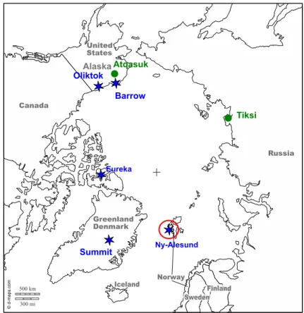
Better understanding of Arctic cloud processes and feedbacks requires long-term and accurate observations (Blanchard et al., 2014; Devasthale et al., 2016). In particular, the knowledge of the vertical cloud structure and phase is crucial for an estimation of the cloud radiative impact (Curry et al., 1996; Shupe and Intrieri, 2004; Liu et al., 2012; Turner et al., 2018). In order to retrieve information on the vertical distribution of clouds and their properties, active remote sensing instruments such as lidars and cloud radars have to be exploited (Protat et al., 2006). However, there are only a few Arctic sites that provide long-term continuous information about the vertical cloud structure using the combination of ground-based remote sensing measurements. These sites are illustrated in Fig. 1.1. Until recently, there were only 4 sites equipped with a variety of instruments including but not limited to a lidar, a cloud radar, a microwave radiometer, and surface radiation and thermodynamic measurement tools, namely Barrow (Alaska; de Boer et al., 2009; Verlinde et al., 2016), Oliktok (Alaska; de Boer et al., 2019), Eureka (Canada; de Boer et al., 2009), and Summit (Greenland; Shupe et al., 2013).
In January 2016 the German Research Foundation started the Transregional Collab-orative Research Center (TRR 172) called "Arctic Amplification: Climate Relevant Atmospheric and Surface Processes, and Feedback Mechanisms (AC)3" (Wendisch et al., 2017). The aim of the (AC)3project is to better understand relations between
all the components of the Arctic climate. Within this project space-borne, air-borne, ship-borne, and ground-based observations are analyzed to improve representation of local-to-global scale processes influencing the Arctic climate in models.
As a part of this project, comprehensive observations of the atmospheric column have been performed at the French-German Arctic Research Base AWIPEV station, operated by the Alfred Wegener Institute Helmholtz Centre for Polar and Marine Research (AWI) and the French Polar Institute Paul Emile Victor (PEV), at Ny-Ålesund. Within the (AC)3 project the instrumentation of the AWIPEV station,
was complemented with a cloud radar in 2016 and, thus, allows for state-of-the-art vertically resolved cloud observations.
Ny-Ålesund (78.92◦N, 11.92◦E) is situated at the coastline of Spitsbergen of the Svalbard archipelago. The Svalbard region is located in the area with the highest warming temperature trend in the Arctic (Susskind et al., 2019). In addition, the Svalbard region is often influenced by distinct synoptic regimes bringing either warm moist air from lower latitudes or cold and dry air circulating in the Arctic area (Dahlke and Maturilli, 2017; Mewes and Jacobi, 2019).
Ny-Alesund Alaska Eureka Tiksi Oliktok Barrow Atqasuk Summit
Figure 1.1: Ground-based Arctic observatories with long-term range re-solved cloud observations. The original map was taken from https://d-maps.com/m/world/arctique/arctique10.pdf. Green circle marks and blue stars show sites with ceilometer and radar-ceilometer observations, respec-tively. The red circle indicates the measurement site analyzed in this thesis.
This thesis is devoted to a characterization of an impact of thermodynamic condi-tions at Ny-Ålesund on cloud microphysical and radiative properties. The investiga-tion is based on state-of-the-art active, passive, and in situ instruments, a numerical weather prediction model and radiative transfer calculations routinely performed within the (AC)3 project for Ny-Ålesund.
1.1
Role of clouds in the radiation budget
The Earth climate is a complex system defined by the energy exchange between space and five climate components, namely atmosphere, hydrosphere, cryosphere, lithosphere, and biosphere (Trenberth and Stepaniak, 2004). The major part of this energy is received from the Sun in the form of electromagnetic waves. On average the Solar irradianceS0 is 1361 W m−2 (Ohmura, 2012). The solar radiation consists
predominantly of shortwave (SW) radiation, which includes near-infrared and visible wavelengths from 0.4–4µm. On the way to the Earth’s surface the solar radiation is partly attenuated by atmospheric components, such as gases, clouds, and aerosols. SW radiation reaching the surface (F↓SW) is partly absorbed by the surface, while
another part is reflected up (F↑SW).
from 4 to 100 µm. The atmospheric components also emit LW radiation. The LW radiation can either reach the top of the atmosphere and escape to the space or be absorbed by atmospheric components and the surface. The down-welling LW radiation reaching the surface is further denoted as F↓LW.
The differences between incoming and outgoing radiation at the surface Q, also known as the surface net radiation budget, indicate how much radiative energy is absorbed by the surface:
Q=F↓SW −F↑SW | {z } QSW +F↓LW −F↑LW | {z } QLW . (1.1)
In the case when Q < 0, more energy leaves the surface and, thus, the surface is radiatively cooled. WhenQ >0 the surface is getting warmed by the radiation. The effect of clouds on the radiation budget is characterized by the so-called cloud radiative effect (CRE). In general, CRE at the surface and at the top of atmosphere are often analyzed. Nevertheless, in this thesis the main focus is on the surface radiation budget because the Arctic warming is more pronounced at the surface (Serreze et al., 2009; Boeke and Taylor, 2018). In addition, Wild and Liepert (2010) showed that the surface radiation budget is a key determinant of the intensity of the hydrological cycle and may influence see and land ice coverage (van den Broeke et al., 2009). Therefore, hereafter only CRE at the surface is considered. The longwave (LW), shortwave (SW) and net CRE are defined as differences between corresponding all-sky and cloud-free radiation budgets according to (Ramanathan et al., 1989): CRESW =QSW −(F↓clr,SW−F↑clr,SW) | {z } QSW clr , (1.2) CRELW =QLW −(F↓clr,LW−F↑clr,LW) | {z } QLW clr , (1.3)
CRE=CRESW +CRELW, (1.4)
where F↓clr,SW, F↓clr,SW, F↑clr,LW and F↑clr,LW are surface down- and upwelling fluxes
for SW and LW, respectively, which would be if the sky were cloud free.
Based on space-borne observations Matus and L’Ecuyer (2017) estimated SW, LW, and net CRE over the globe (Fig. 1.2). The authors showed that on average clouds produce surface radiative cooling of 24.9 W m−2. The strongest cooling was found to occur in the Tropical area. In contrast, the strongest surface radiative warming by clouds is about 20 W m−2 in the polar regions.
Figure 1.2: Annual average SW, LW, and net CRE at the surface. Figure adapted from (Matus and L’Ecuyer, 2017). The numbers indicate global averages of the corresponding CRE.
1.2
Role of clouds in the Arctic warming
The important role of clouds for the global climate was shown in many studies (Taylor et al., 2013; Matus and L’Ecuyer, 2017). First, clouds are the second largest contributor to the surface warming in polar regions in response to the anthropogenic CO2forcing. The surface warming due to green-house gases changes cloud properties
and consequently their radiative effect. The exact response of clouds to the surface warming is not yet clear (Ceppi et al., 2017). Vavrus (2004) noticed that changes in clouds caused by CO2 forcing may be associated with one third of the surface
global warming signal at all latitudes, with up to 40 % in the Arctic region. The cloud-induced temperature response is associated with the enhanced downwelling LW flux at the surface due to the increased presence of low-level liquid-containing clouds. Second, most of the contemporary climate models show that from the top-of-the-atmosphere perspective clouds enhance warming in the Tropical region with a lesser impact in the Arctic region. This indicates, that clouds could be one of the atmospheric components opposing the Arctic amplification at TOA (Taylor et al., 2013; Pithan and Mauritsen, 2014; Block et al., 2019). Third, clouds tend to reduce the temperature gradient between the poles and equator at the surface, while they increase the gradient in the upper troposphere (Taylor et al., 2013).
The role of clouds in the global climate is inextricably linked to other components of the climate and the water cycle. A change in one component often leads to a response in many other components, which, in turn, have a feedback effect on the initially changed component. The feedback effects are especially crucial for the Arctic region having the complex environment characterized by a high seasonal variability of the sea/land ice coverage, frequent temperature inversions, drier air and lower temperatures with respect to the Tropics and mid-latitudes, transitions between polar night and polar day. For instance, the high surface albedo due to ice coverage leads to relatively low SW CRE (Miller et al., 2015), since the clouds and snow-covered surface have similar albedo (Cox et al., 2016). In the longwave, the surface downwelling flux depends on the atmospheric temperature (Cox et al., 2015) and, therefore, in the case of temperature inversions low-level clouds can emit at warmer temperatures than the surface (de Boer et al., 2011).
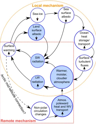
Surface warming LW radiation SW radiation Warmer, moister, cloudier atmosphere Sea-ice Sea surface albedo Land surface albedo Ocean heat storage/ transport Surface turbulent fluxes Atmos. poleward heat and WV transport Non-polar circulation changes Local mechanism Remote mechanism Arctic m id-l atitude conne ction?
Figure 1.3: The schematic diagram of feedback processes induced by the surface warming in the Arctic. Figure adapted from (Boeke and Taylor, 2018). Remote feedback mechanisms are shown within the boarders of a red rectangular box, local feedback mechanisms are inside the orange circle.
Boeke and Taylor (2018) illustrated the feedback mechanisms related to the surface warming in the Arctic region (Fig. 1.3). The authors distinguish two major feedback mechanisms: local and remote. The local mechanism includes processes evolving in the Arctic region while the remote mechanism is related to an atmospheric poleward heat and water vapor transport into the Arctic from the mid-latitude region. Boeke and Taylor (2018) consider the local mechanism as a combination of non-radiative and non-radiative mechanisms. In the non-non-radiative mechanism an increase in the surface temperature is associated with lower sea ice coverage, which leads to more open water that in turn enhances amount of energy collected by the ocean during the extended ice-free season (Serreze et al., 2009; Kapsch et al., 2013). Longer periods of open ocean are related to a warmer, moister, and cloudier atmosphere (Rinke et al., 2013; Palm et al., 2010; Kay and Gettelman, 2009; Mioche et al., 2015; Bennartz et al., 2013). More clouds and water vapor in the atmosphere lead to a stronger green-house effect, which further increases the surface temperature. On the other hand, the same atmospheric changes lead to less SW radiation reaching the surface. Another mechanism affects the surface temperature by the decrease in the surface albedo caused by the sea/land ice retreat. In the case of the decreased surface albedo, the surface absorbs more SW solar radiation, which leads to the surface temperature increase. Hence, the effects of the described mechanisms on the surface temperature due to the SW radiation oppose each other. The surface warming induces the positive albedo feedback, which is partly counteracted by the sun-shading effect by clouds in summer.
The Arctic climate is significantly affected by air masses transported from the mid-latitudes (Graversen and Burtu, 2016; Hwang et al., 2011). A number of studies have already related the air transport and atmospheric rivers to amount of water vapor, cloud properties, and the radiation budget (Hwang et al., 2011; Boisvert et al., 2016; Mortin et al., 2016; Sedlar and Tjernström, 2017; Hegyi and Taylor, 2018). Hegyi and Taylor (2018) reported that the episodes of poleward atmospheric water vapor transport are associated with periods of increased water vapor and cloud cover resulting in enhanced downwelling longwave surface fluxes and reduced surface cooling efficiency. Raddatz et al. (2013) analyzed the impact of cloud coverage and increased water vapor on the longwave downwelling radiation using ground-based observations installed at different sites in the Beaufort Sea–Amundsen Gulf region of the Canadian Arctic. The authors found that the cloud coverage and water vapor explain 84%of the variance of the longwave downwelling radiation, while the remaining 16% are associated with cloud composition, cloud thickness and cloud-base height. Raddatz et al. (2013) estimated differences in the longwave downwelling radiation between cases with typical and maximum values of water vapor. The authors associate the latter to moist intrusion events. The differences are 82 and 95 W m−2 in winter and 38 W m−2and 45 W m−2 in summer for clear sky and cloudy
conditions, respectively. A limited number of studies show that air transportation patterns may influence phase partitioning and amount of liquid in Arctic clouds (Qiu et al., 2018; Tjernström et al., 2019).
A number of recent studies shows an evidence that warmer Arctic temperatures may potentially change non-polar circulation and affect the weather at mid-latitudes (Cohen et al., 2014; Walsh, 2014; Francis and Vavrus, 2015; Boeke and Taylor, 2018; Coumou et al., 2018). However, it is often mentioned that currently there is no consensus on how strong the influence of the Arctic warming on the mid-latitude circulation is.
As depicted in Fig. 1.3, local and remote mechanisms defined by the energy ex-change and the moisture transport, may have a strong impact on the Arctic cloud properties (Cesana et al., 2012; Morrison et al., 2012). It still remains difficult to fully understand the complexity of interactions between different components of the Arctic climate and to assert how they influence the cloud evolution (Vihma et al., 2014). Within the Coupled Model Intercomparison Project Phase 5 (CMIP5) Boeke and Taylor (2016) analyzed 17 climate models and found a larger inter-model spread in the surface radiation budget in the Arctic region. The authors noticed a large divergence in the modeled cloud occurence and CRE among the analyzed models. Differences in cloud occurrence and net surface CRE reached 60% and 40 W m−2, respectively.
1.3
Studies on feedback processes in the Svalbard
region
Ørbæk et al. (1999) showed the uniqueness of the radiation regime in Svalbard. In summer and autumn the radiation budget in the western and southern parts of Svalbard are influenced by the open-ocean climate characterized by the sea fog and the low albedo. In contrast, in winter and spring the radiation regime becomes
more continental similar to the central Svalbard area (Gjelten et al., 2016). Complex terrain in Svalbard leads to local variations in the surface radiation budget. These variations become especially pronounced during the melting and freezing periods. The radiation regime at Ny-Ålesund represents neither the oceanic nor continental types of the Arctic radiation pattern, but rather their combination (Ørbæk et al., 1999): ocean-like radiation climate in summer and autumn, and continental in the winter and spring.
Ohmura (2012) analyzed almost 20 years of surface radiation observations at Ny-Ålesund and found an increase in downwelling LW radiation and surface temperature of 4.9 W m−2 decade−1 and 1.18 ◦C decade−1, respectively. The author stated that the increase in the downwelling LW radiation expected from a sheer temperature increase is 3.4 W m−2 decade−1, while the remaining change should be attributed to changes in the atmospheric components such as greenhouse gases, water vapor feedback, and cloud properties.
Maturilli and Kayser (2016) showed a highly pronounced warming and moistening of the tropospheric column in the Svalbard region. Analyzing a 22-year dataset (1993-2014) from radiosondes the authors found that during winter time there has been a significant increase of atmospheric temperature (up to 3 K per decade) and mean integrated water vapor (+0.83±1.22 kg m−2 per decade). This tendency in
winter is correlated with a strong increase in up- and downward longwave radiation of +11.6±10.9 W m−2 and 15.6±11.6 W m−2, respectively (Maturilli et al., 2015). Dahlke and Maturilli (2017) found a relation between the observed trend in warming and moistening in the winter season in the Svalbard region and the increasing air mass transport through the North Atlantic pathway and reduced flow from the north. Nevertheless, the authors emphasized a lack of understanding of how the circulation shift is connected to other feedback mechanisms including ocean heat transport, sea ice dynamics, and cloud and water vapor radiative effects.
Isaksen et al. (2016) analyzed relationships between the surface air temperature at 5 stations at Spitsbergen and the sea ice concentration. The authors found that the sea ice concentration outside the stations has been reduced on average from 58 to 6% during the period 1997–2015. According to Isaksen et al. (2016), these changes in the sea ice concentration may be important for the local climate. For instance, when the fjord is open, energy is transfered from water to the air and, therefore, convection develops. This transfer is blocked in the case of an ice-covered fjord. In this case, surface inversions can occur (Isaksen et al., 2016). On the regional scale the climate in Svalbard is sensitive to the location of the regional ice edge (Benestad et al., 2002; Isaksen et al., 2016). Isaksen et al. (2016) found a high correlation between the surface air temperature and the sea ice concentration for air masses coming from East and North of Spitsbergen, which indicates an importance of the heat exchange between open water in the Barents Sea and the atmosphere for the atmospheric warming in Spitsbergen. Tetzlaff et al. (2014) analyzed an effect of polynya on the surface temperature in Svalbard. The authors noticed that a larger extent of polynya is related to higher surface temperatures and may increase the potential temperature. The authors argue that polynya extent can lead to strong boundary layer convection, which, in turn, can influence cloud occurrence and precipitation intensity. A number of studies are focused on the energy interactions between the ocean, land, and the atmosphere in the area of Svalbard (Weill et al., 2012; Meyer et al., 2017; Peterson
et al., 2017). Nevertheless, such studies are mostly focused on non-radiative energy transfer effects. Persson et al. (2017) recently showed an analysis of a complete surface energy budget based on the multi year data set from the SHEBA (Surface Heat Budget of the Arctic Ocean) campaign. Such an analysis for Ny-Ålesund requires information on cloud radiative properties, which, until recently, were not available.
The climate at Ny-Ålesund exhibits not only the trends in temperature and humidity but also changes in occurrence of extreme events. For instance, Wei et al. (2016) found significant negative (positive) changes in occurrence of cold (warm) extremes over the last 3 decades. In addition, the authors report that the temperatures of the coldest events increase by 2.3 ◦C decade−1, while temperatures of the hottest
events did not change much. The number of extreme events has also changed (Wei et al., 2016). Cold spells are becoming less frequent (∼–3% decade−1), whereas the occurrence of warm spells increased by ∼ 1.5% decade−1. Wei et al. (2016)
mentioned that the changes in temperatures can be associated with the sea surface temperature and large-scale atmospheric circulation patterns. Yamanouchi (2018) showed a case study with a contrast in cloud conditions and longwave radiation during a transition from cold to warm periods. The authors concluded that the cold periods are associated with low occurrence of clouds and relatively thin clouds, while high cloudiness and thick clouds are typical for periods of warm and moist intrusions. Since the author investigated only a short period, an analysis of longer cloud observations is still needed. Yeo et al. (2018) investigated how the advection of warm and cold air masses affects cloudiness, longwave fluxes at the surface and near-surface temperature at Ny-Ålesund during winter. The authors analyzed a 10-day period in February with alternating warm and cold conditions related to distinct circulation patterns. During cold periods Yeo et al. (2018) observed a reduced cloudiness and down-welling longwave flux of 200-230 W m−2. In contrast, warm
periods were associated with cloud occurrence close to 100 % and enhanced down-welling longwave flux of 300 W m−2. For this study the authors used a ceilometer
and surface radiation measurements and, thus, could not analyze how warm and cold air masses affect microphysical properties of clouds and their radiative effect.
1.4
Coupling of cloud and environmental properties
to SW and LW CRE
One of the most important cloud characteristics affecting the radiative properties of clouds is their phase composition (Shupe and Intrieri, 2004; Sun and Shine, 1994; Yoshida and Asano, 2005; Komurcu et al., 2014). Typically, according to the phase composition clouds are classified into three categories: liquid, ice, and mixed-phase. The first two categories consist purely of liquid and ice particles, respectively. A mixed-phase cloud has liquid and ice phases coexisting within boundaries of the cloud. Long-term in situ observations showed that liquid and ice particles have distinct microphysical properties (Korolev et al., 2003). Liquid droplets have nearly spherical shapes, sizes in the order of 10–20 µm, and the number concentration ranging from4×101 to2×102 cm−3. Ice particles may have a vast variety of shapes
(Bailey and Hallett, 2009; Kneifel et al., 2015). Size of cloud ice also varies in a wide range from 20µm to a few cm. The number concentration of ice particles observed in the atmosphere ranges from 10−8 to 1 cm−3 (Kanji et al., 2017), which is several
order of magnitudes lower than for liquid droplets.
Particles in a cloud have a variety of sizes, which is characterized by a particle size distribution (PSD) N(D), where D is the particle’s size. Typically, a PSD is parameterized by an analytical function, such as generalized Gamma distribution or log-normal distribution, which depend on few parameters. PSD is used to calculate bulk physical properties of cloud particles, e.g. effective radius reff, and liquid and
ice water contents (LWC and IWC):
reff= R∞ 0 r 3N(D)dD R∞ 0 r 2N(D)dD, (1.5) IWC=ρi Z ∞ 0 V(D)Ni(D)dD, (1.6) LWC=ρl Z ∞ 0 V(D)Nl(D)dD, (1.7)
where ρ is the density, r is the radius of a sphere with equal surface area, V is the volume of water in a particle, indexes i and l stand for ice and liquid water, respectively.
A total amount of condensed water in a cloud layer (also known as cloud water path, CWP) can be obtained by integration of vertical profiles of IWC and LWC within the cloud boundaries. For a single mixed-phase cloud layer shown in Fig. 1.4 CWP is defined as follows: CWP= Z hi2 hi1 IWC(h)dh+ Z hl2 hl1 LWC(h)dh. (1.8) In Eq. 1.8 h denotes an altitude with indexes i and l indicating ice and liquid con-taining parts of a cloud, and indexes1and2denote the lower and upper boundaries of a corresponding part of the cloud.
The phase partitioning of a cloud is characterized by liquid water fraction (LWF), which is the ratio of total mass of water in the cloud over CWP:
LWF= hl2 R hl1 LWC(h)dh CWP . (1.9)
In general, an atmospheric profile can have more than one cloud layer. Therefore, often total amounts of ice and liquid water in a vertical profile are characterized by liquid and ice water path (LWP and IWP), respectively:
LWP= Z ∞ 0 LWC(h)dh, (1.10) IWP= Z ∞ 0 IWC(h)dh. (1.11)
Figure 1.4: Schematic diagram of a typical thin single-layer mixed-phase cloud containing a liquid layer close to the cloud top and ice virga below.
Shupe and Intrieri (2004) estimated how different cloud and environment properties influence CRE. The authors considered the atmosphere divided into three layers: the above-cloud atmosphere, the cloud layer, and the below-cloud atmosphere. In this section these layers are denoted by indexesa, c, andbl, respectively. The cloud fraction was assumed to be 1. With this model the authors obtained the following first-order approximation of SW CRE:
CRESW ≈tbsS0cos(z)(1−αs)tcs | {z } cloudy sky −tbsS0cos(z)(1−αs) | {z } clear sky =S0cos(z)tbs(1−αs)(tcs−1), (1.12) where z is the solar zenith angle, αs is the broadband surface albedo, tbs and tcs
are broadband SW atmospheric and cloud transmittances, respectively. The trans-mittances tbs and tcs in Eq. 1.12 include direct and diffuse components. The direct
component is a fraction of the incident radiation passing through the atmosphere without being scattered or absorbed. The diffuse component is a part of the incident radiation that is scattered at least once before reaching the surface (in the case of
tbs) or cloud bottom (in the case of tcs). tbs is defined by properties of atmospheric
gases and aerosols, whiletcs is defined by cloud macro and microphysical properties.
The differences between cloud liquid and ice discussed in Sec. 1.4 result in a di-versity in CRE between liquid, ice, and mixed-phase clouds. Yoshida and Asano (2005) analyzed how LWF influences the radiative properties of clouds in visible and near-infrared parts of the radiation spectrum. The authors showed that for a constant optical cloud thickness LWF does not have a strong effect at visible wave-lengths. At near-infrared wavelengths the influence of LWF is more pronounced. A decrease/increase in LWF lead to lower/higher reflectance and higher/lower absorp-tance. Therefore, the total SW transmittance tcs becomes larger at higher LWF.
According to Eq. 1.12 this leads to more negative CRESW produced by ice clouds
with respect to liquid clouds with the same optical thickness. Nevertheless, many liquid particles often have larger surface area per unit volume than relatively few ice particles and, therefore, liquid clouds tend to have higher optical thickness and, consequently, lower transmittance than ice clouds (Shupe and Intrieri, 2004). Sun and Shine (1994) reported that radiative properties of clouds also depend on how liquid and ice phases are mixed within the cloud boundaries. The simulations performed by the authors showed that the uniform mixing assumption of liquid and
ice within a cloud may lead to about 20% overestimation of the cloud single scatter-ing albedo in comparison to cloud with layered and columnar phase arrangement. The importance of the vertical profiles of liquid and ice for radiative properties of clouds was also shown by Yoshida and Asano (2005). The authors analyzed the sensitivity of cloud SW radiative properties to a change of liquid layer position inside a mixed-phase cloud with fixed liquid and ice water paths. At visible wave-lengths there was no dependence on the position. But reflectance and absorptance of mixed-phase cloud at near-infrared wavelengths are strongly depended on the vertical profile of the phase.
Equation 1.12 shows that beside the cloud microphysical properties, CRESW also
depends on the surface albedo and SZA. Typically, CRESW becomes more negative
with decreasing αs, since there is more contrast between less reflecting surface and
highly-reflecting clouds. Based on measurements from the Arctic Summer Cloud Ocean Study (ASCOS) Sedlar et al. (2011) found that the decrease in αs by 0.01
leads to an increase in the CRESW magnitude by ±1.8 W m−2. Shupe and Intrieri
(2004) showed that for typical late-spring Arctic conditions the decrease in αs by
0.1 changes CRESW to more negative values by about 40 W m−2. SZA, which is the
angle between the zenith and the sun, affects the solar flux reaching the top of the atmosphere. Therefore, when the sun is high in the sky (low SZA), the shading effect of the clouds becomes stronger (Shupe and Intrieri, 2004), i.e. CRESW becomes more
negative.
According to Shupe and Intrieri (2004), LW CRE can be approximated as: CRELW ≈tbl(1−cl)σTa4+tblclσTc4+σTbl4−sσTs4 | {z } cloudy sky − tblσTa4+σTbl4−sσTs4 | {z } clear sky =tblclσ(Tc4−Ta4), (1.13)
where tbl is the broadband LW transmittance of the below-cloud atmosphere; Ta
and Tc are effective temperatures of the above-cloud atmosphere and the cloud,
respectively; σ is the Stefan–Boltzmann constant, cl and s are the broadband
emissivities of cloud and surface, respectively.
Equation 1.13 shows that one of the key parameters defining radiative properties of a cloud in the infrared is the cloud emissivity cl. Smith et al. (1993) showed that
the contribution of the cloud emissivity to the downwelling LW radiation is an order of magnitude larger than the contribution from the cloud reflectance, and, therefore,
cl can be related to the cloud LW transmittance tcl, which is proportional to CWP
(Iacono et al., 2000):
cl ≈1−tcl = 1−e−βdif fκabsCWP, (1.14)
where βdif f is the diffusivity factor typically assumed to be 1.66 (Ebert and Curry,
1992; Garrett et al., 2002) and κabs is the combined liquid and ice phase LW cloud
The cloud absorption coefficientκabsis a sum of the liquid waterκland ice absorption
κi coefficients weighted by the fraction of liquid and ice phase, respectively:
κabs =κlLWF+κi(1−LWF), (1.15)
According to Garrett et al. (2002)κldoes not depend on microphysical properties of
droplets when their sizes are mostly below 10µm. For larger dropletsκl is inversely
proportional to the effective radius ref f. The mass absorption coefficient for ice κi
can be defined as follows (Ebert and Curry, 1992):
κi =
σi
IWC, (1.16)
σi here is the volume absorption coefficient (Ebert and Curry, 1992):
σi =
Z ∞
0
A(D)
4 Qi(D)Ni(D)dD, (1.17) where A is the surface area of an ice particle, Qi is the absorption efficiency of an
ice particle.
Shupe and Intrieri (2004) showed that values of LW CRE range from 0 to 85 W m−2
and depend on the amount of liquid in a column, which is characterized by LWP. The upper limit of CRELW corresponds to clouds with LWP exceeding, depending
on a site, 30–50 g m−2 (Stephens, 1978; Shupe and Intrieri, 2004; Miller et al., 2015;
Ebell et al., 2020). Liquid-containing clouds with LWP exceeding the threshold act as a black body, i.e. cl = 1, and a further increase of LWP does not change their
LW radiative properties.
Since the amount of liquid water is typically related to the atmospheric temperature, Sedlar et al. (2011) investigated how LW CRE is related to the cloud top temper-ature. The authors reported that for cloud base temperatures below –10 ◦C the observed LWP is primarily below 25 g m−2 and CRE
LW ranges from 10–30 W m−2.
For the temperatures above –10 ◦C LWP mostly exceeds 25 g m−2 and CRE
LW
varies from 50 to 85 W m−2.
Ebell et al. (2020) found that the limit in CRELW can be caused by clouds with IWP
exceeding 150 g m−2 based on observations at Ny-Ålesund. This is consistent with
Feofilov et al. (2015), who showed that the ice cloud emissivity does not strongly depend on IWP for clouds with IWP >100−150 g m−2.
1.5
Estimation of CRE from observations
According to Eqs. 1.2 and 1.3 an estimation of CRE requires a knowledge on all-sky SW and LW fluxes (QSW and QLW) and those if the sky were cloud-free (QSW clr
and QLW clr). All sky fluxes can be continuously measured by radiation sensors. In
contrast, QSW clr and QLW clr cannot be directly measured under cloudy conditions
and have to be estimated. Several approaches exist to define the clear sky fluxes. One approach is to substitute QSW clr and QLW clr by the net SW and LW fluxes
Ackerman (2000) developed a technique to identify clear sky scenes based on surface-based observations of total and diffuse SW fluxes. The authors used the identified cases to fit the clear sky flux functions using linear regressions. Regression coeffi-cients are estimated for each day with more than 120 one-minute clear sky samples. A span in the solar zenith angle should be at least 0.4 around the maximum local Sun position. For cloudy days the regression coefficients are linearly interpolated. Long and Turner (2008) proposed a method for continuous estimation of clear sky downwelling LW. The authors identify clear sky cases based on the observed surface downwelling LW flux, air temperature, and relative humidity. F↓clr,LW is
parameter-ized as follows:
F↓LW clr ≈C(ew/Tamb)1/7σTamb4 , (1.18)
where Tamb is the ambient air temperature, ew is the water vapor pressure,and C
is the effective temperature/humidity lapse rate coefficient. The coefficient C is calculated as:
C =k+a(RH)b, (1.19) where coefficients k, a, and b are empirically determined from the identified clear cases.
The methods based on the interpolation of clear sky fluxes to cloudy scenes are straightforward and easy to implement. Since these methods use empirically derived coefficients the results partly include long-term variability in atmospheric gases and aerosols, which have an impact on the atmospheric radiative properties. On the other hand, intra day variability in atmospheric components may introduce additional uncertainties in the coefficient estimations. Furthermore, the methods use only surface observations and are subjects to uncertainties related to variability in vertical profiles of, for instance, water vapor. A major disadvantage of the described methods is the requirement for a sufficient number of clear sky samples, and, for SW, a proper range of zenith angles. For the Arctic region with a high cloud occurrence and polar nights these requirements are often not satisfied.
Another approach of the CRE estimation is based on broadband radiative transfer calculations. Such a method directly accounts for cloud properties as well as influ-ence of any other atmospheric component included in the model. One of the widely used models for the calculation of atmospheric radiative properties is the rapid ra-diative transfer model (RRTMG, Mlawer et al., 1997; Barker et al., 2003). This model requires information on aerosols, surface albedo, temperature and humidity profiles, and cloud microphysics. The model outputs vertical profiles of SW and LW fluxes. In order to estimate the contribution by clouds, the model is run twice with and without clouds for the same other inputs. RRTMG determines the radiative properties of clouds under the plane-parallel assumption, i.e. atmospheric parame-ters are assumed to be homogeneous in horizontal dimensions and vary only in the vertical direction. RRTMG does not take into account three-dimensional radiative effects due to inhomogeneities of surface and broken clouds, multi-scattering effects and atmospheric polarization.
1.6
Observations of cloud properties in the Arctic
For an accurate estimation of CRE with a radiative transfer model, profiles of at-mospheric components are required. Typically, retrieved profiles from ground-based or/and space-borne measurements are used. Satellites with passive and active in-strumentation on-board provide estimation of cloud and aerosol properties, and radiative fluxes in a large-scale perspective (Cesana et al., 2012; Kay et al., 2016; Sedlar and Tjernström, 2017; Wild et al., 2019).
A number of cloud studies is based on passive observations from the MODerate-resolution Imaging Spectroradiometer (MODIS). Two instruments of this type are carried by the Terra and Aqua satellites launched in December 1999 and May 2002, respectively. MODIS has 36 spectral bands from 0.41 to 14.2µm. King et al. (2013) analyzed a decade of MODIS observations and showed that in the Arctic region the average cloud occurrence is about 70%. The authors found 20% more clouds over the Arctic ocean with respect to the land. Based on the algorithm by King et al. (2010), King et al. (2013) analyzed properties of liquid and ice clouds. The authors found a seasonal variability in occurrence of liquid and ice clouds. Over the land liquid clouds were present in 20–30% of profiles during summer months while almost no liquid clouds were detected in winter months. An opposite relation was found for ice clouds with the maximum occurrence of 40% in winter and minimum of 15% in summer. Over the ocean the authors found about a factor of 2 more liquid clouds. The occurrence of ice clouds over the ocean was nearly equivalent in comparison to profiles over the land. Effective sizes of liquid and ice particles were found to be 11–15 and 16–28µm, respectively.
The detection of clouds over the Arctic region using passive space-born instruments is challenging especially over snow covered surfaces and sea ice due to the low con-trast in visible and thermal infrared bands between clouds and underlying surfaces (Liu et al., 2010). For instance, Trepte et al. (2019) analyzed the cloud mask from the Clouds and Earth’s Radiant Energy System (CERES), which is based on a cloud detection algorithm from MODIS. The authors compared the CERES cloud mask with the vertical feature mask from active space-borne observations. The results of the comparison reveal an agreement in cloud cover in 90–99% of cases over snow-free areas for day and night conditions. Over snow-covered areas the detection of clouds agrees in 89–94%and 77–84%of cases during day and night time, respectively (Trepte et al., 2019). It was found that a large part of clouds missed in CERES are clouds with relatively low cloud optical depth (less than 1). In addition, the cloud detection by visible and infrared space-borne instruments exhibits large uncertain-ties during night time conditions due to a low thermal contrast between surface and clouds (Frey et al., 2008; Trepte et al., 2019). Moreover, passive satellite sensors can provide only a limited information on the cloud vertical structure (Zhang et al., 2004) and have difficulties in providing accurate temperature and humidity profiles for the lower atmosphere, which is particularly important for an estimation of the LW downward flux (Wang and Liang, 2009).
Active space-borne instruments can improve the cloud detection and reduce the limi-tations of satellite-based passive instruments. For instance, the Cloud-Aerosol Lidar with Orthogonal Polarization (CALIOP) and the 94 GHz cloud radar installed on the CALIPSO and CloudSat satellites, respectively, are widely used for cloud
in-vestigations. Measurements from CALIOP and the CloudSat radar are not affected by the snow-covered surfaces and the lack of the sunlight during the polar night Mioche et al. (2015). The CloudSat radar can profile almost all non-precipitating clouds. But the CloudSat radar is often not sensitive to thin cirrus clouds, which typically contain relatively small particles. CALIOP is more sensitive to optically thin clouds. Thus, both instruments are typically used in synergy to provide more reliable detection of clouds. Matus and L’Ecuyer (2017) analyzed the cloud fraction on the global scale (gridded with the 2.5◦ x 2.5◦ spatial resolution) utilizing observa-tions from CALIOP and the CloudSat radar for the period from 2007 to 2010. The authors classified cloud profiles to liquid, ice, mixed and multi-layer. The results showed that in the Arctic region the occurrence of clouds is about 75% with 28, 21, 13, and 13% of ice, multi layer, liquid, and mixed-phase clouds, respectively. The authors found that at high latitudes, mixed-phase clouds are less common during winter months as colder temperatures limit the presence of supercooled liquid water. Mioche et al. (2015) analyzed the total cloud occurrence over the entire Arctic region and Svalbard region for the period from 2007 to 2010 and compared the results obtained from different satellite products and ground-based observations. The authors obtained cloud types and properties using the DARDAR algorithm (Delanoe and Hogan, 2010), which is based on combined observations from CALIOP and the CloudSat radar. The results showed that the total cloud occurrence over the Svalbard region is about 5–10% higher than the average over the entire Arctic. In winter and spring this difference reaches 20%. Mioche et al. (2015) also reported that mixed-phase clouds occur in 30% of winter and early spring profiles and 50% during the other seasons. The authors found 10–15% higher occurrence of mixed-phase clouds in the Svalbard region.
Cesana et al. (2012) analyzed ice- and liquid-containing clouds in the Arctic region for the period from 2006 to 2011 using passive and active observations from the CALIPSO satellite. The authors reported that ice-containing clouds were mostly observed at altitudes above 4 km and in the temperature range from -30 to -60 ◦C. Liquid-containing clouds were mostly found in the lowest 3 km at temperatures from -25 to 0◦C. The authors found a spacial variability of the cloud fraction in the Arctic region for different seasons. Liquid-containing clouds have the highest occurrence of 0.65 in summer over the Barents and Greenland seas. In winter and spring the fraction of liquid clouds is about 0.2 over the whole Arctic domain but it may exceed 0.5 in regions affected by the Aleutian and Icelandic Lows.
The detection of low-level clouds from the active space-borne observations has lim-itations (Zygmuntowska et al., 2012; Mioche et al., 2015). The authors compared the retrieved cloud occurrence from CALIOP and the CloudSat radar with ground-based observations and found an underestimation in cloud detection by space-borne instruments of 20%for altitudes between 0.5 and 2 km and 25%below 0.5 km. (Liu et al., 2017) found 25–40%fewer clouds below 0.5 km from the same space-borne in-struments in comparison to ground based inin-struments. Particularly, fewer ice clouds and mixed-phase clouds were observed from space-borne observations between the surface and 1 km height compared to ground-based observations. Blanchard et al. (2014) showed that this limitation is related to the ground clutter contamination and the strong attenuation of the lidar signal, especially by liquid and mixed-phase clouds. In addition, availability of satellite observations for a certain location ranges
from a few times per day to once in several weeks (Winker et al., 2009). Thus, con-tinuous observations are often not available. In addition, satellite instruments have relatively large footprints and coarse spacial resolution. Therefore, inhomogeneities in atmospheric and surface properties are averaged out, which makes it difficult to compare the retrievals based on space and ground-based observations.
Ground-based remote-sensing instruments provide continuous profiling of atmo-sphere with high temporal and spacial resolution. Microwave radiometers allow for temperature and humidity profiling as well as the estimation of total amounts of water vapor and liquid water in a column (Loehnert, 2002; Rose et al., 2005). Active ground-base measurements can be used for the discrimination between liq-uid, ice, and mixed-phase clouds (Shupe, 2007; Illingworth et al., 2007), estimation of IWC Hogan et al. (2006), LWC Frisch et al. (1998), and size of cloud particles (Donovan and van Lammeren, 2001; Frisch et al., 2002; Delanoe and Hogan, 2008). Thus, observations from a cloud radar, lidar, microwave radiometer are widely used to get detailed macro and microphysical properties of clouds (Shupe et al., 2015), which can be used as an input for a radiative transfer model (Shupe and Intrieri, 2004; Dong et al., 2010; Ebell et al., 2011; Turner et al., 2018). The ground-based observations are particularly valuable for the Arctic region, where a large part of the variability in the surface radiation is defined by low-level liquid-containing clouds (Turner et al., 2007), which, as mentioned above, cannot be reliably detected from space. Ground-based radiation sensors are often collocated with a set of atmospheric profilers and, therefore, provide a continuous dataset that can be used to evaluate the results of the used radiative transfer model (Ebell et al., 2011).
Many studies utilized ground-based remote sensing measurements in order to pro-vide statistics on cloud phase, cloud macrophysical and microphysical properties for several Arctic sites (Intrieri et al., 2002; Shupe et al., 2011; Shupe, 2011). A number of cloud studies involved ship- and air-borne sets of instrumentation during inten-sive observation campaigns such as SHEBA program (Uttal et al., 2002) focused on the Beaufort sea region, Mixed-Phase Arctic Cloud Experiment (M-PACE) on the North Slope of Alaska (Verlinde et al., 2007), ASCOS in the central Arctic (Tjern-ström et al., 2014), and the recent ACLOUD/PASCAL campaign in the Svalbard region (Wendisch et al., 2019).
Shupe et al. (2011) analyzed cloud properties at five observatories in the Arctic, namely Atqasuk, Barrow, Eureka, Summit and Ny-Ålesund. The authors showed that in general the total annual cloud occurrence among all these stations varies from 58-83%. The highest occurrence of clouds was observed in autumn and ranged from 80 to almost 100%, while the lowest cloud occurrence of∼60%was typically observed in winter and spring. Shupe et al. (2011) found an unique shift in the cloud annual cycle at Eureka due to distinct meteorological patterns. At Eureka there are less low-level summer clouds and more low- and mid-level winter clouds.
Shupe (2011) analyzed cloud phase at Barrow, Eureka, and for the SHEBA cam-paign. The authors reported that ice clouds were the predominant type of clouds with the occurrence up to 60–70%at all sites. Liquid phase was observed 56%of the time at Barrow and during the SHEBA campaign but much less frequent at Eureka (30%). It was also shown that the water saturation conditions were reached less frequently at the Eureka station, which lead to lower occurrence of liquid-containing clouds at this site in comparison to the other Arctic sites. Shupe et al. (2015) found
that the monthly mean LWP ranged from 20–110 g m−2 at Barrow and was higher than the monthly mean values of IWP varying from 5 to 70 g m−2 for all seasons.
The highest LWP was observed at Barrow in late summer and early autumn while the largest IWP was observed in early autumn and middle of spring. For the Bar-row dataset Shupe et al. (2015) found that the monthly median effective radius of ice particles is about 35 µm throughout a year. The median effective size of liquid particles was typically from 7 to 10 µm.
Shupe and Intrieri (2004) investigated the influence of cloud phase on SW and LW radiation analyzing the data from the SHEBA field camp based on an ice-breaking ship for the period from 1997 to 1998. The authors used the microphysical profiles retrieved from ground-based observations and applied the Santa Barbara Discrete Ordinate Radiative Transfer (DISORT) Atmospheric Radiative Transfer (SBDART) algorithm (Ricchiazzi et al., 1998). The results showed that annually averaged CRELW and CRESW for liquid-containing clouds were 52 and –21 W m−2,
respectively. For pure ice clouds CRELW and CRESW were found to be 16 and –
3 W m−2, respectively, indicating that liquid containing clouds are more radiatively
effective than ice clouds for the dataset analyzed by Shupe and Intrieri (2004). Dong et al. (2010) analyzed 10-years of cloud observations at Barrow and found that on average the net CRE at Barrow is 3.5 W m−2. The authors reported that for regions located more to the south from the Barrow station the annual Net CRE is negative (e.g. –17.9 W m−2, Alaska 60◦N) while to the north it becomes more
positive (e.g. 26.9 W m−2 during the SHEBA experiment). Such a latitudinal dependence of CRE may result from the combined effect of SZA and the surface albedo. For the Summit station Miller et al. (2015) found the annually averaged CRE of 33 W m−2. CRE is positive during a year and shows a low seasonal variability, which is opposite to other Arctic sites where CRE is negative in summer.
Until summer 2016 the AWIPEW station at Ny-Ålesund was equipped only with one profiling instrument – ceilometer. Based on observations from the ceilometer Shupe et al. (2011) analyzed macrophysical properties of clouds at Ny-Ålesund, such as cloud occurrence, persistence, and cloud base height. An analysis of microphysical and radiative properties of clouds, similar to the one conducted for the Barrow and Summit stations, was not possible because there was no measurements available from a cloud radar.
1.7
Focus and scientific questions of the thesis
Clouds are one of the major components of the Arctic climate and their accurate representation in climate models is crucial for analysis of the radiation budget. Un-derstanding of clouds is especially important for the Arctic regions experiencing the fastest temperature increase over the last decades. The Svalbard island is currently the only place with continuous active and passive atmospheric profiling located in such a region. Even though, the Ny-Ålesund station is well equipped with instru-ments continuously monitoring the atmosphere during several decades, the literature review given in this chapter shows a lack of detailed cloud characterization at Ny-Ålesund.
The atmosphere in Svalbard and clouds in particular are strongly affected by the long-distance air transport. Even though there is a general evidence how the air transport influences clouds in the Svalbard area, more information is required in order to link the cold and warm air intrusions with clouds and their radiative effect. This link is one of the missing parts towards a complete surface energy budget similar to those recently carried out by Persson et al. (2017) for the SHEBA campaign. Profiling of cloud microphysical properties at Ny-Ålesund was not possible because only one profiling instrument (ceilometer) was used until summer 2016, when a cloud radar was installed within the (AC)3 project in order to close the gap in cloud
observations.
The aim of the current study is to answer the following questions:
• What characteristics do clouds have at Ny-Ålesund?
• How good can a numerical weather prediction model represent cloud properties at Ny-Ålesund?
• How do moist and dry conditions influence cloud properties including occur-rence, cloud types, IWP, and LWP at Ny-Ålesund?
• How do changes in cloud properties due to moist and dry conditions influence CRE at Ny-Ålesund?
• Do long-term observations of the atmospheric state at Ny-Ålesund show sig-nificant trends in the occurrence of moist and dry conditions over the last decades?
• If there are trends in the occurrence of moist and dry conditions at Ny-Ålesund, what is their impact on LW CRE?
In order to answer these questions, continuous atmospheric observations taken from June 2016 to October 2018 at Ny-Ålesund within the (AC)3 project were used to
analyze cloud properties, surface radiation, fluxes, and atmospheric states. A state-of-the-art set of passive, active, and in situ instruments utilized in this study is de-scribed in Chapter 2. The widely used processing algorithm Cloudnet was applied by the Finnish Meteorological Institute to the observations. Based on the cloud categorization from Cloudnet, a cloud classification and microhysical retrievals were used to estimate properties of ice and liquid cloud particles. Chapter 3 shows gen-eral statistics of cloud properties and gives a comparison of the observations and a numerical weather prediction model. Profiles of the retrieved cloud properties as well as thermodynamic properties of the atmosphere were used by Ebell et al. (2020) as an input for RRTMG simulations. In Chapter 4 cloud properties and CRE from RRTMG are related to moist, dry, and normal conditions at Ny-Ålesund. Long-term trends in occurrence of moist and dry conditions are analyzed in Sec. 4.5.
Since RRTMG requires profiles of cloud properties, the estimated CRE is only avail-able from June 2016 onwards. Nyeki et al. (2019) showed that effects of cloud on the surface radiation can be deducted from LW flux observations and cloud frac-tion, which, as was shown by Long and Ackerman (2000); Long and Turner (2008), can also be approximated from the surface flux measurements. In order to relate
the long-term trends in atmospheric water vapor to changes in CRE, an algorithm estimating CRE from available long-term observations is developed. The algorithm is based on neural networks and uses different combinations of inputs, such as sur-face LW fluxes, cloud base detection from a ceilometer, brightness temperatures from a microwave radiometer, surface temperature and humidity. Chen et al. (2006) have already shown that neural networks are capable of the LW CRE estimation. The authors used cloud fraction, cloud base height, and cloud base temperature retrieved from the lidar/radar synergy. In this study, the radar was not available before June 2016. A long-term lidar dataset is available for Ny-Ålesund (Maturilli and Ebell, 2018) but the dataset is not homogeneous because lidars of different types were used (Sec. 2.3). Therefore, even though the developed algorithm is similar to the approach by Chen et al. (2006), different input parameters were used. The de-veloped method and its results are presented in Chapter 5. Finally, in Chapter 6 a summary and an outlook for the future research are presented.
Parts of this thesis have been published:
• Nomokonova T., Ebell K., Löhnert U., Maturilli M., Ritter C., and O’Connor E. (2019), Statistics on clouds and their relation to thermodynamic conditions at Ny-Ålesund using ground-based sensor synergy. Atmospheric Chemistry
and Physics, vol. 19, no.6, pages 4105-4126, doi: 10.5194/acp-19-4105-2019.
Parts of this publication are mainly used in Chapters 2 and 3.
• Nomokonova T., Ebell K., Löhnert U., Maturilli M., and Ritter C. (2019), The influence of anomalous atmospheric conditions at Ny-Ålesund on clouds and their radiative effect. Atmospheric Chemistry and Physics Discussions, 1-34, doi: 10.5194/acp-2019-985. This publication is mainly used in Chapters 2 and 4.
Datasets used for the analysis in this thesis have been published:
• Nomokonova T., and Ebell, K. (2019), Cloud microphysical properties re-trieved from ground-based remote sensing at Ny-Ålesund (10 June 2016 – 8 October 2018). University of Cologne, PANGAEA,https://doi.pangaea.
de/10.1594/PANGAEA.898556.
• Nomokonova, T., Ritter, C., Ebell, K. (2019), HATPRO microwave radiometer measurements at AWIPEV, Ny-Ålesund (2016 – 2018). PANGAEA, https:
Instrumentation and data products
In this study a set of passive, active, and in situ instrumentation continuously run-ning at the AWIPEV observatory was used. An overview of the measurement site is shown in Fig. 2.1. A cloud radar and a microwave radiometer are installed at the roof on the AWIPEW observatory building, while a ceilometer and radiation sensors are mounted on the ground about 100 m away from the building. In addition, a number of data products derived from the measurements or models are utilized. In this chapter, a review of the instruments, data products, and models as well as a short description of the measurement principles and retrieval methods are given. Information for this chapter is partly taken from Nomokonova et al. (2019b) and Nomokonova et al. (2019a).2.1
Cloud radar
In this thesis two 94 GHz cloud radars, JOYRAD-94 and MIRAC-A (Fig.2.2), of the University of Cologne are used. Both radars are of the same type and were manufac-tured by Radiometer Physics GmbH (RPG). JOYRAD-94 and MIRAC-A are ver-tically pointing radars and utilize frequency-modulated continuous wave (FMCW) signals. Küchler et al. (2017) showed the details on the operational principle and signal processing for JOYRAD-94. JOYRAD-94 was installed at the AWIPEV sta-tion on 10th of June 2016 where it was operated until its replacement by MIRAC-A in July 2017. In this study radar data until 8 October 2018 are used. Main hardware parameters and operational settings of the radars are shown in Table 2.1.
The used cloud radars are active instruments which emit radiation in form of pe-riodical frequency-modulated signals (also known as chirps) to the atmosphere and receive a signal returned by atmospheric scatters. Ranging in FMCW radars is per-formed by measuring frequency differences between the transmitted and received signals, which are proportional to the distance at which the scatters are located. The returned power Pr measured by the radars is defined by properties of scatters
and by radar specifications. In order to get a quantity independent on the radar characteristics,Pr is usually converted to so called equivalent radar reflectivity
fac-tor (Z, radar reflectivity hereafter):
Figure 2.1: Overview of the AWIPEV measurement site at Ny-Ålesund.
Figure 2.2: The 94 GHz cloud radars JOYRAD (a) and MIRAC-A (b) mounted on the roof of the AWIPEV station at Ny-Ålesund.
Z =|Kw|−2CaPrr2, (2.1)
where |Kw| is the dielectric factor of liquid water, Ca is the radar constant, which
takes into account the radar specifications, andris range from the radar to the scat-ters. Z has units of mm6 m−3 but often logarithmic units dBZ= 10 log10(mm6 m−3) are used.
For spherical cloud particles with sizes much smaller than the wavelength, Z is proportional to the sixth raw moment of the size distribution:
Z ∼
Z ∞
0
D6N(D)dD. (2.2) Here D is the size of a scatter and N(D)dD is a number of particles in a unit volume with sizes ranging from D to D+dD. Equation 2.2 shows that in the case of Rayleigh scattering the radar reflectivity is mostly dominated by a presence of larger particles (Hogan et al., 2006).