Accepted Manuscript
Nonparametric estimation of dynamic discrete choice models for time
series data
Byeong U. Park, L´eopold Simar, Valentin Zelenyuk
PII:
S0167-9473(16)30259-6
DOI:
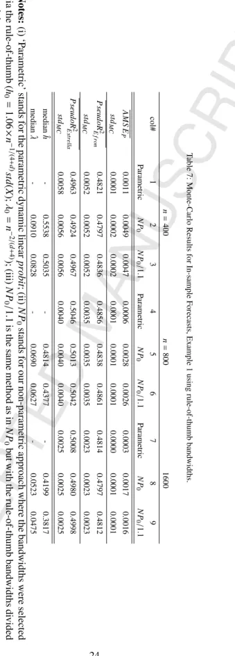
http://dx.doi.org/10.1016/j.csda.2016.10.024
Reference:
COMSTA 6374
To appear in:
Computational Statistics and Data Analysis
Received date: 21 May 2015
Revised date:
25 October 2016
Accepted date: 25 October 2016
Please cite this article as: Park, B.U., Simar, L., Zelenyuk, V., Nonparametric estimation of
dynamic discrete choice models for time series data.
Computational Statistics and Data
Analysis
(2016), http://dx.doi.org/10.1016/j.csda.2016.10.024
This is a PDF file of an unedited manuscript that has been accepted for publication. As a
service to our customers we are providing this early version of the manuscript. The manuscript
will undergo copyediting, typesetting, and review of the resulting proof before it is published in
its final form. Please note that during the production process errors may be discovered which
could affect the content, and all legal disclaimers that apply to the journal pertain.
Nonparametric Estimation of Dynamic Discrete Choice Models for
Time Series Data
Byeong U. Parka, L´eopold Simarb, Valentin Zelenyukc,∗ aDepartment of Statistics, Seoul National University, Korea
bInstitut de Statistique, Biostatistique et Sciences Actuarielles, Universit´e Catholique de Louvain, Belgium cSchool of Economics and Centre for Efficiency and Productivity Analysis (CEPA) at The University of Queensland, Australia
Abstract
The non-parametric quasi-likelihood method is generalized to the context of discrete choice models for time series data, where the dynamic aspect is modeled via lags of the discrete dependent variable appearing among regressors. Consistency and asymptotic normality of the estimator for such models in the general case is derived under the assumption of stationarity with strong mixing condition. Monte Carlo examples are used to illustrate performance of the proposed estimator relative to the fully parametric approach. Possible applications for the proposed estimator may include modeling and forecasting of probabilities of whether a subject would get a positive response to a treatment, whether in the next period an economy would enter a recession, or whether a stock market will go down or up, etc.
Keywords: Nonparametric quasi-likelihood, local-likelihood, dynamic probit, forecasting
1. Introduction
Discrete response (or choice) models have received substantial interest in many areas of research. Since the in-fluential works of McFadden (1973, 1974) and Manski (1975), these models have become very popular in economics, especially microeconomics, where they were elaborated on and generalized in many respects. Some very interesting applications of such models are also found in macroeconomic studies where one needs to take into account time series aspects of data. Typical applications of the time series discrete response models deal with forecasting of economic recessions, the decisions of central banks on interest rate, movements of the stock market indices, etc. (See Estrella and Mishkin (1995, 1998), Dueker (1997, 2005), Russell and Engle (1998, 2005), Park and Phillips (2000), Hu and Phillips (2004), Chauvet and Potter (2005), Kauppi and Saikkonen (2008), de Jong and Woutersen (2011), Harding and Pagan (2011), Kauppi (2012) and Moysiadis and Fokianos (2014) to mention just a few.)
The primary goal of this work is to develop a methodology for non-parametric estimation of dynamic time series discrete response models, where the discrete dependent variable is related to its own lagged values as well as other regressors. The theory we develop in the next two sections is fairly general and can be used in many areas of research.
The reason for going non-parametric, at least as a complementary approach, is very simple, yet profound: The parametric maximum likelihood in general, and probit or logit approaches in particular, yield inconsistent estimates if
the parametric assumptions are misspecified. Many important works addressed this issue in different ways, e.g., see
Cosslett (1983, 1987), Manski (1985), Klein and Spady (1993), Horowitz (1992), Matzkin (1992, 1993), Fan et al. (1995), Lewbel (2000), Honore and Lewbel (2002), Fr¨olich (2006), Dong and Lewbel (2011), Harding and Pagan (2011), to mention just a few.
The main contribution of our work to existing literature is that we generalize the method of Fan et al. (1995) to the context that embraces time series aspects and in particular the case with lags of the (discrete) dependent variable
∗Correspondence to: 530, Colin Clark Building (39), St Lucia, Brisbane, Qld 4072, Australia; tel:+61 7 3346 7054.
appearing among the regressors. Such a dynamic feature of the model is very important in practice. For example, in weather forecasting, one would also naturally expect that the lagged dependent variable, describing whether the previous day was rainy or not, may play a very important role in explaining the probability that the next day will also be rainy. Another example of the importance of the dynamic component among the explanatory factors in discrete response models can be found in the area of forecasting economic recessions (Dueker (1997) and Kauppi and Saikkonen (2008)).
We derive the asymptotic theory for the proposed estimator under the assumption of stationarity with strong
mixing condition (in the spirit of Masry (1996)). Our approach is different from and compliments to another powerful
non-parametric approach based on the Nadaraya-Watson estimator (e.g., see Harding and Pagan (2011)). Specifi-cally, we use an alternative estimation paradigm—the one based on the non-parametric quasi-likelihood and the local likelihood concepts—which have well-known advantages over the least squares approach for the context of discrete response models. Furthermore, we consider and derive the theory for the local linear fit, which is known to pro-vide more accurate estimation of a model than the local constant approach and is more convenient for estimation of
derivatives or marginal effects of the regressors on (the expected value of) the response variable.
It is also worth noting here that a related approach (a special case of ours) was used by Fr¨olich (2006) who considered the local likelihood method in the case of a binary logit-type regression model with both continuous and discrete explanatory variables, in a cross-section set up. Specifically, Fr¨olich (2006) provided very useful and convincing Monte Carlo evidence about superior performance of the local likelihood logit relative to parametric logit for his set up (cross-sectional), but without deriving asymptotic properties of the resulting estimators. Our work encompasses the work of Fr¨olich (2006) as a special case, and, importantly, allows for time series nature of the data, including the dynamic aspect, and provides key asymptotic results for this set up that appears to be missing in the literature. A natural extension to our work would be to also allow for non-stationarity (e.g., as in Park and Phillips (2000)), which is a subject in itself and so we leave it for future research.
Our paper is structured as following: Section 2 outlines the general methodology, Section 3 outlines the the-oretical properties of the proposed estimator, Section 4 discusses the choice of bandwidths, Section 5 provides some Monte Carlo evidence, while the Appendix provides further details.
2. General Methodology
Suppose we observe (Xi,Zi,Yi),1≤i≤n,where{(Xi,Zi,Yi)}∞
i=−∞is a stationary random process. We assume
that the process satisfies a strong mixing condition, as described in detail in the next section. The response variable
Yi is of discrete type. For example, it may be binary taking the values 0 and 1. The vector of covariatesXi is of
d-dimension and of continuous type, whileZiis ofk-dimension and of discrete type. The components of the vector
Ziare allowed to be lagged values of the response variable. For example,Zi =(Yi−1, . . . ,Yi−k). Our main interest is
to estimate the mean function
m(x,z)=E(Yi|Xi=x,Zi=z).
We employ the quasi-likelihood approach of Fan et al. (1995) to estimate the mean function. It requires two
ingre-dients. One ingredient is the specification of a quasi-likelihoodQ(·,y), which is understood to take the role of the
likelihood of the mean whenY = yis observed. It is defined by∂Q(µ,y)/∂µ =(y−µ)/V(µ), whereV is a chosen
function for the working conditional variance modelσ2(x,z) ≡var(Y|X =x,Z =z) =V(m(x,z)), where here and
below (X,Z,Y) denotes the triple that has the same distribution as (Xi,Zi,Yi). The other ingredient is the specification
of a link functiong. The link function should be strictly increasing. In a parametric model where it is assumed that
g(m(x,z)) takes a parametric form, its choice is a part of the parametric assumptions. Thus, a wrong choice would
jeopardize the estimation ofm. In nonparametric settings, its choice is less important. One may take simply the
identity function as a link, but one often needs to use a different one. One case is where the target functionmhas
a restricted range, such as the one whereY is binary so thatmhas the range [0,1]. A proper use of a link function
guarantees the correct range.
With a link functiongand based on the observations{(Xi,Zi,Yi)}n
i=1, the quasi-likelihood of the function f
defined by f(x,z) =g(m(x,z)) is given byPn
i=1Q(g−1(f(Xi,Zi)),Yi). Let (x,z) be a fixed point of interest at which
we want to estimate the value of the mean functionmor the transformed function f. We apply a local smoothing
data points change smoothly on the scale of the distance to the point (x,z), while in the space of discrete covariates
they take some discrete values, one for the caseZi=zand the others forZi,z. Specifically, we use a product kernel
wi
c(x)×wid(z) for the weights of (Xi,Zi) around (x,z), where wi c(x)= d Y j=1 Khj(xj,X i j), wid(z)= k Y j=1 λI(Z i j,zj) j .
Here,I(A) denotes the indicator such thatI(A)=1 ifAholds, and zero otherwise,Kh(u,v)=h−1K(h−1(u−v)) is a
symmetric kernel functionK, while bandwidthshjandλjare real numbers such that 0≤λj ≤1. The above kernel
scheme for the discrete covariatesZiis due to Racine and Li (2004) and is in the spirit of Aitchison and Aitken (1976).
Note that this approach is different from a special case whereλis set to be zero (e.g., see Harding and Pagan (2011)
for the case of Nadaraya-Watson estimator). Indeed, as pointed out by Racine and Li (2004), by setting bandwidths of the discrete variables to zero, the “estimator reverts back to the conventional approach whereby one uses a frequency estimator to deal with the discrete variables”, i.e., one performs separate estimation for each group identified by the discrete variable (but with the same bandwidths for the continuous variables). In fact, an important particular case
is whenλj = 1, implying that the discrete regressor jis irrelevant (see Hall et al. (2007)). Thus, allowing for the
flexibility that eachλjcan be anywhere between 0 and 1 is important both for generalizing the asymptotic theory as
well as for the applied work. One can also generalize further by allowing more adaptive bandwidths, e.g., allowing for bandwidths of some or all continuous variables to vary across groups defined by some or all discrete variables, as was
discussed in Li et al. (2016). Here we proceed with Aitchison-Aitken/Racine-Li type kernel for the sake of simplicity.
Furthermore, note that approximating f(Xi,Zi) locally by f(x,z) does not make use of the link function and
the quasi-likelihood since it gives an estimator that results from using the local least squares criterion. We take the following local approximation which is linear in the direction of the continuous covariates and constant in the direction of the discrete covariates.
f(u,v)' f˜(u,v)≡ f(x,z)+ d X
j=1
fj(x,z)(uj−xj), (2.1)
wherefj(x,z)=∂f(x,z)/∂xj. To estimate f(x,z) and its partial derivatives fj(x,z), we maximize n−1Xn i=1 wi c(x)wid(z)Q g−1 β0+ d X j=1 βj(Xij−xj) ,Yi , (2.2)
with respect toβj,0 ≤ j ≤ d. The maximizer ˆβ0 is the estimator of f(x,z) and ˆβj are the estimators of fj(x,z),
respectively. Then, one can estimate the mean functionm(x,z) by inverting the link function,g−1( ˆβ0).
Our theory given in the next section tells us that the asymptotic properties of the estimators do not depend
largely on the choice of link functiongas long as it is sufficiently smooth and strictly increasing. This is mainly
because the estimation is performed locally. Approximating locally the functiong1(m(x,z)) or g2(m(x,z)) for two
different linksg1andg2does not make much difference. Although, it is sometimes suggested to use the canonical link
when it is available since it guarantees convexity of the objective function (2.2) so that the optimization procedure is numerically stable.
When the likelihood of the conditional mean function is available, one may use it in place of the
quasi-likelihood Qin the description of our method. This is particularly the case when the response Y is binary. In the
latter caseP(Y =y|X=x,Z=z)=m(x,z)y[1−m(x,z)]1−y,y=0,1. Thus, one may replaceQ(µ,y) by
`(µ,y)=ylog µ
1−µ
!
+log(1−µ).
see Fr¨olich (2006)), then one maximizes, instead of (2.2), n−1Xn i=1 wi c(x)wid(z)` g−1 β0+ d X j=1 βj(Xij−xj) ,Yi =n−1 n X i=1 wi c(x)wid(z) Yi β0+ d X j=1 βj(Xij−xj) −log1+eβ0+Pdj=1βj(Xij−xj). (2.3)
If one uses theprobitlinkg(t)= Φ−1(t) whereΦdenotes the cumulative distribution function of the standard normal
distribution, then one maximizes
n−1Xn i=1 wic(x)wid(z) " Yilog Φβ0+Pdj=1βj(Xij−xj) 1−Φβ0+Pdj=1βj(Xij−xj) +log 1−Φ β0+ d X j=1 βj(Xij−xj) # . (2.4)
Also note that whenY is binary, our local likelihood approach is related to the binary choice model formulated as
Yi=If(Xi,Zi)−εi≥0. (2.5)
Thus, the model is a non-parametric extension of the parametric model considered by de Jong and Woutersen (2011) where it is assumed that f is a linear function andεi is independent of (Xi,Zi). Whenεihas a distribution function G, thenm(x,z)=P(εi≤ f(x,z))=G(f(x,z)). Thus, the non-parametric binary choice model (2.5) leads to our local
likelihood with linkg =G−1. For example, the local likelihood (2.3) is obtained whenεihas the standard logistic
distribution with distribution function of the formG(u)=eu(1+eu)−1, while the one at (2.4) corresponds to the case
whereεihas the standard normal distribution. In this respect, the choice of a link function amounts to choosing an
error distribution in the binary response model. 3. Theoretical Properties
3.1. Assumptions
Here, we collect the assumptions for our theoretical results. Throughout the paper we assumehj ∼n−1/(d+4),
which is known to be the optimal rate for the bandwidthshj. For the weightsλjwe assumeλj ∼ n−2/(d+4). This
assumption is mainly for simplicity in the presentation of the theory. Basically, it makes the smoothing bias in the space of the continuous covariates and the one in the space of the discrete covariates be of the same order of magnitudes.
The joint distribution of the response variableYand the vector of discrete covariatesZhas a discrete measure
with a finite support. For the kernelK, we assume that it is bounded, symmetric, nonnegative, compactly supported,
say [−1,1]. Without a loss of generality we also assume it integrates to one, i.e.,´ K(u)du=1.
We also assume the marginal density function of Xis supported on [0,1]d, and the joint density p(x,z) of
(X,Z) is continuous in x for allz, and is bounded away from zero on its support, while the conditional variance
σ2(x,z)=var(Y|X =x,Z=z) is continuous inx. We also assume the mean functionm(x,z) is twice continuously
differentiable inxfor eachz. These are standard conditions for kernel smoothing that are modified for the inclusion
of the vector of discrete covariatesZ.
Now, we state the conditions on the stationary process{(Xi,Zi,Yi)}. The conditional density of (Xi,Zi) given Yiexists and is bounded. The conditional density of (Xi,Zi,Xi+l,Zi+l) given (Yi,Yi+l) exists and is bounded. For the
mixing coefficients
α(j)≡ sup
A∈F0
−∞,B∈Fj∞
whereFb
a denotes theσ-field generated by{(Xi,Zi,Yi) :a≤i≤b}, we assume
α(j)≤(const)(jlogj)−(d+2)(2d+5)/4, (3.1)
for all sufficiently large j. The assumptions on the conditional densities are also made in Masry (1996) where some
uniform consistency results are established for local polynomial regression with strongly mixing processes. Our
condition (3.1) on the mixing coefficients is a modification of those assumed in Masry (1996) that fits for our setting.
We also assume typical conditions that are needed for the theory of the quasi-likelihood approach. Specifically, we assume that the quasi-likelihoodQ(µ,y) is three times continuously differentiable with respect toµfor eachyin the support ofY,∂2Q(g−1(u),y)/∂u2<0 for alluin the range of the mean regression function and for allyin the support
ofY, the link functiongis three times continuously differentiable,Vis twice continuously differentiable,Vandg0are
bounded away from zero on the range of the mean regression function, and the second and the third derivatives ofg
are bounded.
3.2. Main Theoretical Results
In this section we give the asymptotic distribution of ˆf(x,z). Letpdenote the density function of (X,Z) and
fjk(x,z)=∂2f(x,z)/(∂xj∂xk). Here and in the discussion below, we treat (x,z) as fixed values of interest at which we
estimate the function f. For the vectorz, we letz−jdenote the (k−1)-vector which is obtained by deleting the jth
entry ofz.
Define ˆα0= fˆ(x,z)−f(x,z) and ˆαj=hj( ˆfj(x,z)−fj(x,z)) for 1≤ j≤d. By the definition of ˜f at (2.1), it
fol-lows that the tuple ( ˆαj: 0≤j≤d) is the solution of the equation ˆF(α)=0, where ˆF(α)=( ˆF0(α),Fˆ1(α), . . . ,Fdˆ (α))>,
ˆ F0(α)=n−1 n X i=1 wi cwid Yi−mi( ˜f,α) V(mi( ˜f,α))g0(mi( ˜f,α)), ˆ Fj(α)=n−1 n X i=1 wi cwid Xi j−xj hj Y i−mi( ˜f,α) V(mi( ˜f,α))g0(mi( ˜f,α)), 1≤ j≤d,
andg0is the first derivative of the link functiong. Here, we suppressxandzinwi
candwid, and also write for simplicity
mi(θ,α)=g−1 θ(Xi,Zi)+α0+ d X j=1 αj Xi j−xj hj ,
for a functionθdefined onRd×Rk. As approximations of ˆF
jfor 0≤j≤d, let F∗ 0(α)=E " wi cwid mi(f,0)−mi(f,α) V(mi(f,α))g0(mi(f,α)) # , F∗ j(α)=E wicwid Xi j−xj hj m i(f,0)−mi(f,α) V(mi(f,α))g0(mi(f,α)) , 1≤j≤d.
Note thatmi(f,0)=E(Yi|Xi,Zi). The following lemma demonstrates that ˆF
j(α) are uniformly approximated byF∗j(α)
forαin any compact set.
Lemma 3.1. Assume the conditions stated in subsection 3.1. Then, for any compact setC ⊂Rd
sup{|Fˆj(α)−F∗j(α)|:α∈ C}=Op
n−2/(d+4)(logn)1/2,
Under the condition thatQ(g−1(u),y) is strictly convex as a function ofu, the vectorF∗(α)≡(F∗
0(α),F1∗(α), . . . ,F∗d(α))>
is strictly monotone as a function ofα. Thus, the equationF∗(α)=0has a unique solutionα=0. This and Lemma 3.1
entail ˆα →0in probability. The convergence of ˆαand the following lemma justify a stochastic expansion of ˆα. To
state the lemma, we define some terms that approximate the partial derivatives ˆFj j0(α)≡∂Fj(α)/∂αj0. Let
˜ F00(α)=E wicwid V(mi( ˜f,α))g0(mi( ˜f,α))2 , ˜ F0j(α)=E Xi j−xj hj wi cwid V(mi( ˜f,α))g0(mi( ˜f,α))2 , 1≤ j≤d, ˜ Fj j0(α)= E Xi j−xj hj Xi j0−xj0 hj0 wi cwid V(mi( ˜f,α))g0(mi( ˜f,α))2 , 1≤ j,j0≤d,
and form a (d+1)×(d+1) matrix ˜F(α) with these terms.
Lemma 3.2. Assume the conditions stated in subsection 3.1. Then, for any compact setC ⊂Rd
sup{|Fˆj j0(α)−F˜j j0(α)|:α∈ C}=Op
n−2/(d+4)(logn)1/2,
0≤ j,j0≤d.
We note that ˜Fj j0(α) are continuous functions ofα. Thus, it follows that ˜Fj j0( ˆα∗) = F˜j j0(0)+op(1) for any
stochastic ˆα∗such thatkαˆ∗k ≤ kαˆk. This with ˆF( ˆα)=0and Lemma 3.2 implies
ˆ
α=−F˜(0)−1Fˆ(0)+op(n−2/(d+4)). (3.2)
In the above approximation we have also used the fact ˆF(0) = Op(n−2/(d+4)) which is a direct consequence of the
following lemma.
Lemma 3.3. Assume the conditions stated in subsection 3.1. Then,
(nh1× · · · ×hd)1/2 " σ2(x,z)p(x,z) V(m(x,z))2g0(m(x,z))2 #−1/2 D−1/2 1 × Fˆ(0)−V(m(x,zp))(xg,0z(m)(x,z))2 12e0 d X j=1 fj j(x,z)h2j ˆ u2K(u)du+e 0b(x,z) !# d −→ N(0,Id+1),
whereId+1denotes the(d+1)-dimensional identity matrix,e0is the(d+1)-dimensional unit vector(1,0, . . . ,0)>,D1
is a(d+1)×(d+1)diagonal matrix with the first entry being(´ K2(u)du)dand the rest(´ K2(u)du)d−1´u2K2(u)du and b(x,z)=g0(m(x,z)) × k X j=1 λj X z0 j,zj,z0j∈Dj p(x,z−j,z0j) p(x,z) [m(x,z−j,z 0 j)−m(x,z)].
Also, it follows thatF˜(0) = −D2·V(m(x,z))−1g0(m(x,z))−2p(x,z)+o(1), whereD2is a(d+1)×(d+1)diagonal matrix with the first entry being1and the rest´ u2K(u)du.
In Lemma 3.3, we see that the asymptotic variance does not involve the discrete weightsλj. This is because
the contributions to the variance by the terms in ˆFj(0) withwid <1 are negligible in comparison to those by the terms
withwi
d = 1 which corresponds to the case whereZi = z. This is not the case for the asymptotic bias. Note that
the conditional mean of theith term in ˆFj(0) given (Xi,Zi) contains the factormi(f,0)−mi( ˜f,0)=g−1(f(Xi,Zi))− g−1( ˜f(Xi,Zi)). ForZi=z, it equalsg−1(f(Xi,z))−g−1(f(x,z)+Pd
j=1fj(x,z)(Xij−xj)), so that the leading terms come
from the approximation of f along the direction ofXi. However,ZiwithZi ,zalso contribute nonnegligible bias.
Note that in this case we have
mi(f,0)−mi( ˜f,0) ' g−1 f(x,Zi)+ d X j=1 fj(x,Zi)(Xij−xj) −g−1 f(x,z)+ d X j=1 fj(x,z)(Xij−xj) ' g−1(f(x,Zi))−g−1(f(x,z)),
where the error of the first approximation is of ordern−2/(d+4) and the second one of order n−1/(d+4) for Xi in the
bandwidth range, i.e., forXiwithwi
c > 0. When the discrete kernel weightswid are applied to the differences, the
leading contributions of the differences are made byZi withPkj=1I(Zij , zj) = 1 and they are of the magnitude
λj∼n−2/(d+4).
From (3.2) and Lemma 3.3, we have the following theorem.
Theorem 3.1. Assume the conditions stated in subsection 3.1. Then, we have
(nh1× · · · ×hd)1/2 "g0(m(x ,z))2σ2(x,z) p(x,z) #−1/2 × ˆ K2(u)du!−d/2 fˆ(x,z)−f(x,z)−1 2 d X j=1 fj j(x,z)h2j × ˆ u2K(u)du−b(x,z) # d −→ N(0,1).
The theorem stated above tells us that the asymptotic distribution of the estimator ˆf is normal and invariant
under the misspecification of the conditional variance σ2(x,z) in terms of the mean function m(x,z), that is, the
asymptotic distribution does not change even ifσ2(x,z)),V(m(x,z)). A close investigation into the term ˜F(0) and
Lemma 3.3 reveals that the termV(m(x,z)) cancels out in the asymptotic variance of ˆf(x,z). As for the asymptotic
bias of the estimator, the termPd
j=1fj j(x,z)h2j
´
u2K(u)du/2 typically appears in nonparametric smoothing over a
continuous multivariate regressor, while the termb(x,z) is due to the discrete kernel smoothing.
4. Bandwidths
The asymptotic theory summarized in previous section is derived for any bandwidths satisfying the mentioned convergence rates, namely hj ∝ n−1/(d+4) and λj ∝ n−2/(d+4), and so, theoretically, they are not influenced when
they are scaled by a constant. In practice, however, the selection of bandwidths is an important matter. Usually, a small variation of the bandwidths do not lead to dramatic changes in estimation results (as is also confirmed in simulations below), but big changes in the bandwidths may be influential. Indeed, very large values for bandwidths can lead to oversmoothing of the data. On the other hand, choosing very small values may result in overfitting. For a discrete variable, taking very large bandwidth (1 in the limit) would be equivalent to ignoring or omitting the discrete variable. On the other hand, taking very small bandwidth for a discrete variable would be equivalent to treating the
thus possible that the choice of the bandwidths in practice may influence not only quantitative but also qualitative conclusions implied by the regression estimates and so this choice must be made carefully.
To implement our estimator one may use various approaches already suggested in the literature. Investigating which one of them is the best is by large a subject in itself that is beyond the scope of this paper and so we limit our discussion here to a few practical tips and explanations of what we used in the simulation sections that follow.
A simple and very fast way, which is quite commonly used in the field of kernel-based estimation, is to start with some types of rules-of-thumb. For example, at various instances below, we make use of the so-called
Silverman-type rule-of-thumb adapted to the regression context, which for a continuous variableXis given by
h0(X)=1.06×n−1/(4+d)σˆX, (4.1)
where ˆσXis the empirical standard deviation of observations on variableX. Similarly, for a discrete variable, we make
a use of the following rule-of-thumb bandwidth value
λ0=n−2/(d+4). (4.2)
Another, more sophisticated and much more computer intensive, approach is to use a data driven procedure to select
the bandwidthsoptimally with respect to some desirable criterion. One of the most popular of such approaches,
for example, is based on the so-called leave-one-out cross-validation (CV) criterion, e.g., where one selects such
bandwidthshcvandλcvthat jointly maximize the following likelihood-based cross-validation criterion
CV(h, λ) = 1 n n X i=1 `g−1fˆh(,λ−i)(Xi,Zi),Yi, (4.3)
where ˆfh(−i,λ)(Xi,Zi) is the estimate of the function f at the point (Xi,Zi) computed from the ‘leave-theith
observation-out’ sample with the value (h, λ) for the bandwidths. (Here, it might be worth noting that if there are no continuous
regressors, theCVchoice ofλwill converge to zero at the raten−1.)
The statistical properties of CV bandwidth selectors in kernel regression with only continuous type covariates were first studied by H¨ardle et al. (1988). See also Hall and Johnstone (1992) for smoothing parameter selection based
on various empirical functionals. It is widely known that a CV bandwidth ˆhconverges to its optimum, sayhopt, in the
sense that (ˆh−hopt)/hopt =op(1), which means ˆh=Op(n−1/(d+4)) in our context. Racine and Li (2004) extended this
result to the case where there is a discrete covariate. They proved that both the bandwidth selectors ˆhand ˆλbased on
a CV criterion have the properties that (ˆh−hopt)/hopt =op(1) and (ˆλ−λopt)/λopt =op(1), wherehopt andλopt are
the corresponding theoretically optimal bandwidths such thathopt n−1/(d+4)andλ
opt n−2/(d+4). One may prove
the same results in our context so that the bandwidth selectors ˆh and ˆλthat minimize the CV criterion (4.3) have
asymptotically the magnitudesn−1/(d+4)andn−2/(d+4), respectively.
Besides the rule-of-thumb and the CV bandwidths, many other approaches suggested in the literature can also be used for our estimator (as long as they satisfy the theoretical rates). For example, additional flexibility can be added by allowing more adaptive bandwidths, e.g., some or all bandwidths for continuous variables may be allowed to vary with some or all of the discrete variables (e.g., see Li et al. (2016)).
It should be also noted that maximization of CV function or its variations often is a relatively challenging task, especially for high dimensions and large samples and typically requires numerical optimization. The rule-of-thumb estimates of the bandwidths are often used for the starting values to initiate the iterations of the numerical
optimization. Depending on a sample,CV(h, λ) may have multiple local minima, some of which are ‘spurious’ in the
sense described by Hall and Marron (1991) in the context of density estimation (also see Park and Marron (1990) for
related discussion). Here, this could lead to too smallh, leading to overfitting or an even worse value ofhsuch that
the local linear estimator is not defined; so, imposing lower bounds onhcould prevent such degenerate solutions.
It is also worth noting that selecting bandwidths via CV is the most computer intensive part of all the estimation procedure here. For example, an estimation of a model of the type described in Example 2 and 3 below with a
pre-selected bandwidth took about 0.1 minute and 1 minute for a sample ofn=100 and a sample ofn=1000, respectively
(on machine with 1.3 GHz Intel Core i5 with 8GB 1600 MHz DDR3). Meanwhile, for the same models, obtaining
n=1000 respectively. While such timing seems not so excessive for one or even several estimations, it is prohibitively
expensive to do for each of the many replications in the Monte Carlo (MC) simulations. Therefore, some simplified strategy for bandwidths estimation in the MC study is needed.
To expedite the computations in the simulations below, we use the following strategy: for each scenario and
different types of sample sizes, we estimate CV-optimal bandwidths by minimizing (4.3) (using several starting values
including (4.1) and (4.2)) and compared the performance of the results to those obtained by using the rule-of-thumb bandwidths. We did this only for the in-sample forecasts. Our experiments generally suggested that the performance of our nonparametric approach with CV-bandwidths are very similar to those for rule-of-thumb bandwidths and so we only use the rule-of-thumb bandwidths (because they are much faster) for the MC evaluation of the out-of-sample forecasts. Even with such non-optimal but appropriate and very fast to compute bandwidths, the results from the nonparametric model are much better than from the parametric model when the latter is misspecified and very similar when the latter happens to be correctly specified.
5. Simulations
In this section we illustrate how the procedure behaves in finite samples in terms of in-sample and out-of-sample forecasts, considering three simulated situations. In the first scenario, the parametric probit with linear index (hereafter linear probit) is the true model, i.e., the idea is to see how our estimator behaves when the “world” is linear.
We expect that the nonparametric estimator will be less accurate than thecorrectlyspecified parametric model, but it
is interesting to see whether the loss is substantial.
For the second scenario we have a model where the linear probit is wrong (we add a quadratic term) and we expect that our estimator brings more accurate information on the data generating process than the linear probit. In the third example, we intensify the nonlinearity by considering a periodic index, to see if the nonparametric estimator is able to capture the essence of the true model and how much it improves upon the linear probit.
In all the examples below we generate the time series according to the following simple binary dynamic probit model Yi∼binomialP(Yi=1|x i,yi−1) , i=1, . . . ,n, (5.1) where P(Yi=1|xi,yi −1)= Φ(ψ(xi,yi−1)), i=1, . . . ,n, (5.2)
withXi ∼ U(lb,ub) and we initialize the series withy
0 =0. The three examples presented below involve different
specifications ofψ(xi,yi−1).
For each replication, we estimated several measures of quality or ‘goodness of fit’ to get an understanding of relative performance of the parametric linear probit and our nonparametric approach. Specifically, to measure the quality of the in-sample forecasts, the first basic measure that we used is the approximate mean squared error between the true and the estimated probabilities, i.e.,
AMS EP= 1 n n X i=1 P(Yi=1|xi,yi −1)−bP(Yi=1|xi,yi−1) 2 . (5.3)
This measure is very useful but limited by the fact thatP(Yi = 1|xi,yi
−1) is available only in simulated data and so
many other practical alternatives were proposed and used in the literature (e.g., see Estrella (1998) and references cited there in) and we use some of them here.
Specifically, the second measure of fit we use is in the spirit of Efron (1979), defined as
PseudoR2
E f ron=1−AMS Eo/AMS Ec, (5.4)
whereAMS Eois the approximate mean squared error between the observationYiand the estimated probability, i.e.,
AMS Eo= 1 n n X i=1 Yi−bP(Yi=1|xi,yi −1) 2 , (5.5)
whileAMS Ecis the approximate mean squared error of the naive estimator given by unconditional mean ¯Y, i.e., AMS Ec= 1 n n X i=1 Yi−Y¯2, (5.6)
and so, in a sense, this measure presents performance of an estimator relative to the naive approach of just looking at
the unconditional mean of the sample, ¯Y(i.e., proportions of observations whereYi=1).
Finally, we also use the Pseudo-R2proposed (in parametric context) by Estrella (1998), defined as
PseudoR2Estrella=1− log(L ∗ u) log(L∗ c) !−2 log(L∗ c) , (5.7) where log(L∗
u) is the value of the maximized (parametric or nonparametric) log-likelihood of the full (unconstrained)
model and log(L∗
c) is the value of maximized log-likelihood of the constrained (or naive) model with only the intercept.
In the tables below we present the averages of these measures overM=100 replications. The relatively small
number of replications is dictated by the high cost of computations (due to optimization of CV criterion), but to sense
the variability of these measures across all the replications (b =1, ...,M), we also present the Monte Carlo standard
deviations, i.e., stdMC = v u t 1 M(M−1) M X b=1 go fb−go f2,
wherego fbis a goodness of fit measure among those presented above andgo f is its average overMreplications.
For the same computational reasons, we mainly focus on MC results for n ∈ {25,50,100,200}, where we
used both the CV and the rule-of-thumb bandwidths. We also experimented with larger samples but using only the fast-to-compute bandwidths based on the rule-of-thumb described above and slight deviations from it (e.g., changing them by about 10%) and the conclusions were generally the same. We provide such evidence in Appendix B (for
n∈ {400,800,1600}). In this Appendix B we also provide typical plots of histograms of the bandwidths over 100 MC
replications, which helps sensing the variability of CV and rule-of-thumb bandwidths across MC replications.
To investigate how the two models behave for the ‘out-of-sample’ forecasts, we useAMS EPas described above
except that the averaging is made not overnobservations, but over the ‘out-of-sample’ observations (which were not
used in the model estimation) and their forecasts. Specifically, here we investigated the results for the forecasts one-period ahead and two-one-periods ahead, by starting the forecasting 10 one-periods before the end of the series, supposing that
the value ofXiis known at least two periods in advance (i.e., we can imagineXis an exogenous variableX∗,i−` with
lag`≥2), and then rolling forward. This gave 9 out-of-sample forecasts for each type of (one-period ahead and
two-periods ahead) forecasts of probabilities, which were then compared to the true probabilities. Also note that for the one-period ahead forecast, the value ofyiis available for forecastingYi+1, and so we can computeP(Yi+1=1|xi
+1,yi)
directly. Meanwhile, for the two-periods ahead forecasts, we use the iterated approach of Kauppi and Saikkonen (2008)–we decompose the forecast according to the conditional probabilities, considering the two possible paths for
Yi+1, which is either 0 or 1. Specifically, we have
P(Yi+2=1|xi
+1,xi+2,yi)= P(Yi+1=1|x
i+1,yi)P(Yi+2 =1|xi+2,yi+1=1)
+P(Yi+1 =0|xi+1,yi)P(Yi+2=1|xi+2,yi+1=0), (5.8)
where the true values of all the probabilities on the right hand side are given by our probit model (5.2). We then plug in our estimates to obtain our two-periods ahead forecasts. This strategy was used in all the examples presented below. Some remarks on the bandwidths selection are in order. Ideally, one may want to compute optimal bandwidths in each replication. Due to computational burden, however, researchers often choose to use a simple way to select bandwidths in each replication of an MC scenario, e.g., using some rule-of thumb bandwidths or even the same
band-widths over all replications (within the same scenario and the same sample size), e.g., median bandband-widths obtained for a pilot of 20 or so replications. We tried all these approaches and noticed that selecting optimal bandwidths for each replication may actually yield less favorable results (e.g., higher average AMSE) than using a median of optimal bandwidths for a sub-set of replications or even relative to the rule-of-thumb bandwidths. This is due to the fact that CV sometimes gave too small or too large bandwidths, thus overfitting or oversmoothing the true models relative to the case when the same median bandwidths were used for the same scenario and sample size.
Finally, note that for the out-of-sample forecasts, the new bandwidths must be estimated with each rolling for-ward–because (i) new information is added and (ii) the sample size changes. Doing so with CV is too computationally intensive, and so we had to resort to a simplified strategy, where we just used the rule-of-thumb bandwidths described in the previous section, recomputing them for any changes in the sample.
5.1. Simulated Example 1
In this first example we generate the time series according to the simple dynamiclinearindex function given
by
ψ(xi,yi−1)=β0+β1xi+β2yi−1, i=1, . . . ,n, (5.9)
For the results summarized in the tables and figures below, we setβ0 = −0.2,β1 = −0.75 ,β2 = 2, lb =
−3, ub = 3, while also noting that qualitatively similar conclusions were also obtained with other values of these
parameters. We use figures below to visually illustrate performance of parametric and nonparametric approaches for
a more or less typical MC replication (withn=100), while tables below summarize results from 100 MC replications
for different sample sizes.
Of course,a priori, we expect that, on average, the parametric linear probit approach must perform better than
the nonparametric approach (although in some replications we also observed the opposite), because the latter does not use the information about the (correct) linearity of the true model while the former does. In particular, this is reflected in the faster convergence rates of the parametric approach relative to the nonparametric one (in our case, it is
√nfor parametric vs.n2/5for the nonparametric with one continuous variable). This expectation is confirmed in most
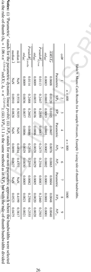
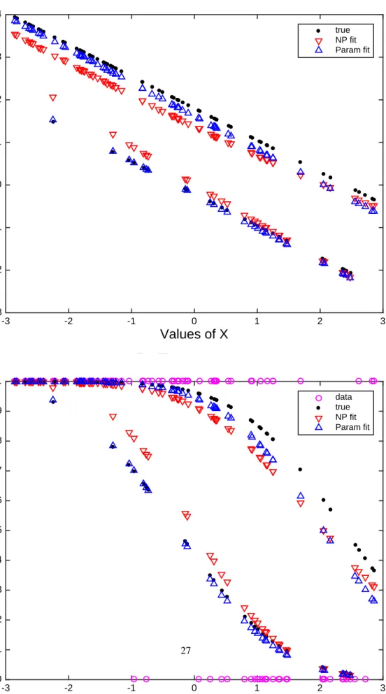
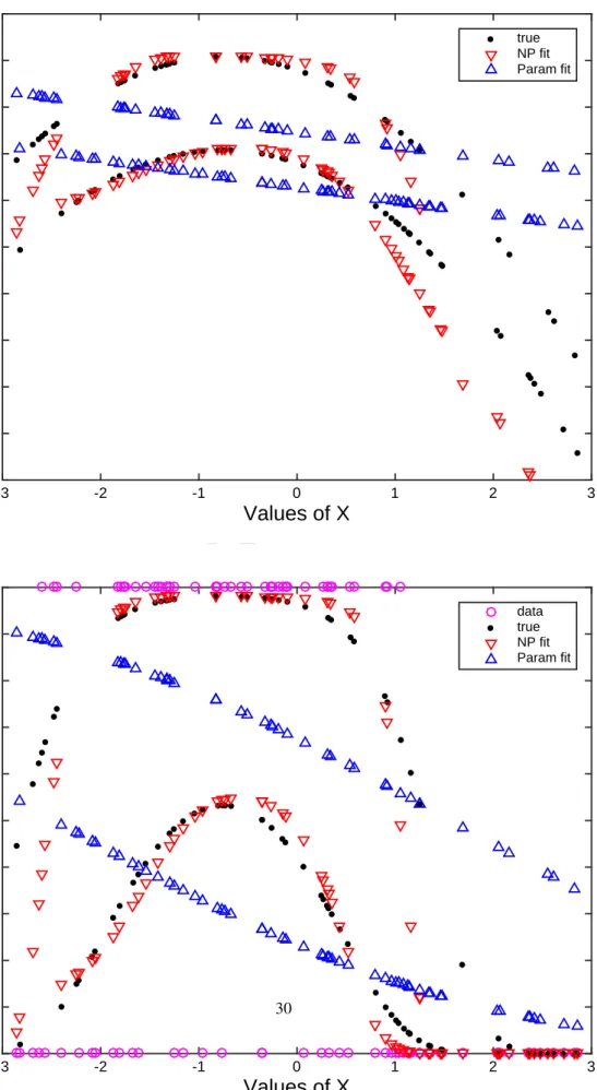
of MC replications, summarized in Table 1 and Table 2. Figure 1 presents results for such estimation in one typical
replication withn = 100 observations for the index function in the upper panel and the corresponding probabilities
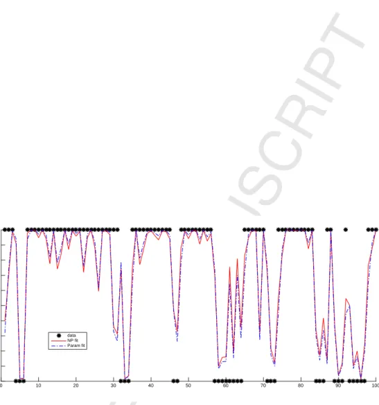
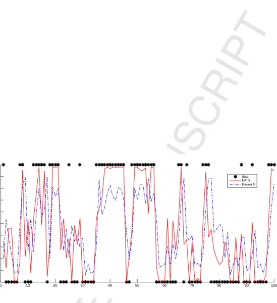
along with the realizations ofY (0 or 1, depicted with circles) in the lower panel. Moreover, Figure 2 displays the
time series view of the behavior of the 100 in-sample forecasts of the two approaches, where we plot the realizations
ofYin the simulation (0 or 1, depicted with dots) against the respective time-series of probabilities estimated via the
parametric and nonparametric approaches using CV bandwidths (depicted with broken and solid curves).
Table 1 presents the averages of measures of goodness-of-fit over 100 replications and one can draw several conclusions from this scenario. First, note that the parametric approach by using correct parametric information is performing substantially better than the nonparametric method in terms of the in-sample forecasting of the true
prob-abilities, withAMS EPfor both converging to zero as sample size increases. Despite this, however, the nonparametric
method performs similarly well, and sometimes slightly better than the correctly specified parametric approach in
terms of both of thePseudo−R2measures. Also note that forn=25 andn =50, the nonparametric approach with
the rule-of-thumb bandwidths performed better than the same approach with CV bandwidths in terms ofAMS EP,
but the latter outperformed for the larger samples (n = 100 andn = 200), although both were already fairly close
to converging to zero. The nonparametric approach with the rule-of-thumb bandwidths and with CV bandwidths
showed very similar performance in terms ofPseudo−R2measures, except forn=25 where the estimator with CV
bandwidths outperformed. Also note that in all cases except whenn=25, the median ofhwas very large, suggesting
that in most cases the CV approach to bandwidths selection was able to recognize that the true model is linear by
yieldinghthat is well beyond the range of simulatedx. Overall, the Table 1 confirms that for the in-sample forecasts,
the nonparametric estimator behaves well in the in-sample forecasts although it is not using the information about linearity, which happened to be correct in this example.
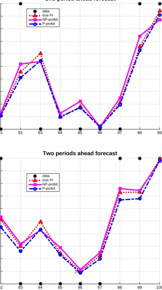
Let us now look at the performance in terms of out-of-sample forecasts. The results for one replication with
n = 100 are presented in Figure 3, which displays the true probabilities and their out-of-sample forecasts, for
one-period and two-one-periods ahead. The forecasts seem particularly good for both the (correctly specified) parametric estimator and the nonparametric estimators. Table 2 presents the averages over 100 replications and confirms that
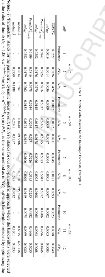
Table 1: Monte-Carlo Results for the In-sample Forecasts, Example 1. n = 25 n = 50 n = 100 n = 200 col# 1 2 3 4 5 6 7 8 9 10 11 12 Parametric N P 0 N P cv Parametric N P 0 N P cv Parametric N P 0 N P cv Parametric N P 0 N P cv A M S E P 0.0227 0.0276 0.0424 0.0102 0.0182 0.0211 0.0045 0.0121 0.0093 0.0023 0.0078 0.0040 st d M C 0.0019 0.0014 0.0036 0.0009 0.0009 0.0017 0.0004 0.0005 0.0007 0.0002 0.0003 0.0003 P seud oR 2 E fr on 0.5842 0.5724 0.6816 0.5037 0.5095 0.5085 0.5073 0.5043 0.5072 0.4806 0.4796 0.4846 st d M C 0.0252 0.0176 0.0270 0.0145 0.0117 0.0178 0.0096 0.0093 0.0108 0.0065 0.0063 0.0068 P seud oR 2 E st rel la 0.6109 0.5816 0.6978 0.5244 0.5234 0.5271 0.5226 0.5195 0.5253 0.4982 0.4966 0.5050 st d M C 0.0252 0.0179 0.0262 0.0153 0.0124 0.0184 0.0106 0.0099 0.0119 0.0075 0.0069 0.0080 median ˆ h -0.9634 1.3361 -0.8448 89.8606 -0.7330 595.8548 -0.6375 622.1360 median ˆ λ -0.2759 0.1188 -0.2091 0.1257 -0.1585 0.0532 -0.1201 0.0233 Notes: (i) ‘P arametric’ stands for the parametric dynamic linear pr obit ;(ii) N P 0 stands for our non-parametric approach where the bandwidths were selected via the rules of thumb ( h 0 = 1 . 06 × n − 1 / (4 + d ) st d ( X ); λ 0 = n − 2 / ( d + 4) ); (iii) N P cv is the same method as in N P 0 but with bandwidths selected by optimizing the (lea ve-one-out) CV in each replication;
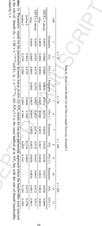
Table 2: Monte-Carlo Results for the Out-of-sample Forecasts, Example 1. n = 25 n = 50 n = 100 n = 200 col# 1 2 3 4 5 6 7 8 9 10 11 12 Parametric N P0 N P0 / 1 . 1 Parametric N P0 N P0 / 1 . 1 Parametric N P0 N P0 / 1 . 1 Parametric N P0 N P0 / 1 . 1 A M S EP (1-ahead) 0.0327 0.0764 0.0771 0.0129 0.0381 0.0381 0.0048 0.0211 0.0205 0.0023 0.0089 0.0087 st dM C 0.0029 0.0090 0.0092 0.0014 0.0056 0.0056 0.0007 0.0032 0.0033 0.0003 0.0016 0.0016 A M S EP (2-ahead) 0.0368 0.0697 0.0720 0.0144 0.0327 0.0326 0.0047 0.0166 0.0174 0.0025 0.0081 0.0081 st dM C 0.0037 0.0085 0.0085 0.0017 0.0049 0.0048 0.0005 0.0028 0.0030 0.0004 0.0012 0.0012 median ˆh -0.9634 0.8759 -0.8448 0.7680 -0.7330 0.6664 -0.6375 0.5796 median ˆλ -0.2759 0.2509 -0.2091 0.1901 -0.1585 0.1441 -0.1201 0.1092 Notes: (i) ‘P arametric’ stands for the parametric dynamic linear pr obit ;(ii) N P0 stands for our non-parametric approach where the bandwidths were selected via the rule-of-thumb ( h0 = 1 . 06 × n − 1 / (4 + d ) st d ( X ); λ0 = n − 2 / ( d + 4) ); (iii) N P0 / 1 . 1 is the same method as in N P0 but with the rule-of-thumb bandwidths di vided by 1.1.
approaches tend to zero as the sample size increases. Also note that the nonparametric approach gave similar results whether using the rule-of-thumb bandwidths or their smaller (divided by 1.1) versions, which was the case for both the one-period ahead and the two-periods ahead forecasts.
5.2. Simulated Example 2
Here we simulate the same model as in Example 1, except that we also add a quadratic term in x. The true
index is now given by
ψ(xi,yi−1)=β0+β1xi+β2yi−1+γx2i,
whereβ0 andβ1 are the same as above and γ = −0.5. As expected we will observe a poor performance of the
incorrectly specified linear probit approach and we will see that the nonparametric approach approximates this model fairly well.
The results for the estimation in one typical replication withn =100 observations are shown in Figure 4 for
the index function (upper panel) and the probabilities (lower panel) and in Figure 5 for the 100 in-sample forecasts over the time series. These figures do not require much comment: the fit of the nonparametric approach here is clearly much better than that of the parametric linear probit.
Table 3 confirms the conclusions from the figures, presenting a summary of the MC results for the in-sample forecasts over 100 replications. One can see that the nonparametric approach outperforms parametric in all the
in-sample goodness-of-fit measures–having substantially lower AMS EP and substantially higher PseudoR2
Estrella and PseudoR2
E f ron, even for such small samples asn=25 andn=50. Also note that in terms ofAMS EP, the difference
in performance increases with sample size, as for the nonparametric approach it tends to zero while for the parametric
approach it seems to rather quickly converge to a positive value near 0.05 rather than zero. In a sense, it is an
illustration of the so-called ‘root-n inconsistency’. It is also worth noting that the nonparametric approach with
rule-of-thumb bandwidths showed significantly better performance in terms ofAMS EPfor smaller samples (n =25
andn = 50) and very similar performance in the larger samples, relative to the nonparametric approach with CV
bandwidths estimated in every replication. On the other hand, their performance was almost identical in terms of the
PseudoR2
EstrellaandPseudoR2E f ronfor all the sample considered.
We now turn to the out-of-sample forecasts of this example. The superior performance of the nonparametric approach relative to the parametric linear probit approach is also confirmed here. The results for one typical replication are shown in Figure 6, which illustrates how the nonparametric out-of-sample forecasts (with CV bandwidths) follow rather well the true probabilities, both in the one-period and the two-periods ahead forecasts. Meanwhile, Table 4 presents the summary over 100 replications confirming the same conclusions as drawn from the figure. Specifically, one can see that the nonparametric approach, as expected, is performing substantially better than the parametric approach in terms of both (one-period and two-periods) out-of-sample forecasts of the true probabilities: An exception
is for the smallest sample case (n = 25) where performance is somewhat similar, while already for n = 50 the
difference inAMS EP became about two-fold, while about 4-times and 6-times forn = 100 andn = 200. This is
becauseAMS EPfor the nonparametric approach tends to zero while for the linear parametric model it appears to be
converging to a positive (misspecification) bias around 0.05. Also note that reducing the bandwidths by about 10%
from the rule-of-thumb values almost did not change the results and certainly did not change the conclusions.
5.3. Simulated Example 3
In this last example we generate the time series according to the following dynamic index function
ψ(xi,yi−1)=β0+sin(β1xi+β2yi−1), i=1, . . . ,n. (5.10)
Note that the index function is also nonlinear in parameters and so it is not so simple to approximate it just by adding a quadratic term in the linear index as would have been possible in the preceding example. Also note that the discrete variable is also inside the sin-function and so its impact on the dependent variable is more complicated than just a vertical parallel shift. For the results presented below we hadβ0=−0.2,β1=−1.75 ,β2=2.
Figure 7 illustrates the results for the estimation for one of the replications, withn =100 observations, for
the index function (upper panel) and the probabilities (lower panel), meanwhile Figure 8 displays results in time series perspective for the 100 in-sample forecasts for this same replication. As should be expected, all figures show
Table 3: Monte-Carlo Results for the In-sample Forecasts, Example 2. n = 25 n = 50 n = 100 n = 200 col# 1 2 3 4 5 6 7 8 9 10 11 12 Parametric N P0 N Pcv Parametric N P0 N Pcv Parametric N P0 N Pcv Parametric N P0 N Pcv A M S EP 0.0572 0.0336 0.0447 0.0561 0.0214 0.0267 0.0552 0.0141 0.0138 0.0539 0.0090 0.0078 st dM C 0.0017 0.0020 0.0030 0.0009 0.0009 0.0015 0.0007 0.0006 0.0007 0.0004 0.0004 0.0005 P seud oR 2 Efr on 0.2950 0.5345 0.5364 0.3117 0.5336 0.5397 0.3025 0.5340 0.5696 0.2825 0.5063 0.5286 st dM C 0.0176 0.0155 0.0238 0.0119 0.0094 0.0145 0.0093 0.0085 0.0097 0.0061 0.0053 0.0066 P seud oR 2 Est rel la 0.3175 0.5704 0.5771 0.3284 0.5761 0.5877 0.3189 0.5820 0.6276 0.2963 0.5561 0.5889 st dM C 0.0195 0.0155 0.0237 0.0127 0.0097 0.0157 0.0101 0.0087 0.0102 0.0065 0.0059 0.0075 median ˆh -0.9634 1.1000 -0.8448 0.8885 -0.7330 0.6854 -0.6375 0.5635 median ˆλ -0.2759 0.2490 -0.2091 0.1110 -0.1585 0.0669 -0.1201 0.0385 Notes: (i) ‘P arametric’ stands for the parametric dynamic linear pr obit ;(ii) N P0 stands for our non-parametric approach where the bandwidths were selected via the rules of thumb ( h0 = 1 . 06 × n − 1 / (4 + d )st d ( X ); λ0 = n − 2 / ( d + 4)); (iii) N Pcv is the same method as in N P0 but with bandwidths selected by optimizing the (lea ve-one-out) CV in each replication;
Table 4: Monte-Carlo Results for the Out-of-sample Forecasts, Example 2. n = 25 n = 50 n = 100 n = 200 col# 1 2 3 4 5 6 7 8 9 10 11 12 Parametric N P 0 N P 0 / 1 . 1 Parametric N P 0 N P 0/ 1 . 1 Parametric N P 0 N P 0/ 1 . 1 Parametric N P 0 N P 0 / 1 . 1 A M S E P (1-ahead) 0.0935 0.0868 0.0880 0.0659 0.0321 0.0310 0.0639 0.0165 0.0156 0.0571 0.0106 0.0099 st d M C 0.0050 0.0094 0.0094 0.0039 0.0031 0.0031 0.0031 0.0017 0.0016 0.0024 0.0010 0.0010 A M S E P (2-ahead) 0.0959 0.0767 0.0770 0.0703 0.0327 0.0322 0.0736 0.0178 0.0167 0.0653 0.0122 0.0113 st d M C 0.0049 0.0093 0.0093 0.0045 0.0035 0.0035 0.0037 0.0022 0.0020 0.0026 0.0012 0.0011 median ˆ h -0.9634 0.8759 -0.8448 0.7680 -0.7330 0.6664 -0.6375 0.5796 median ˆ λ -0.2759 0.2509 -0.2091 0.1901 -0.1585 0.1441 -0.1201 0.1092 Notes: (i) ‘P arametric’ stands for the parametric dynamic linear pr obit ;(ii) N P 0 stands for our non-parametric approach where the bandwidths were selected via the rule-of-thumb ( h 0 = 1 . 06 × n − 1 / (4 + d ) st d ( X ); λ 0 = n − 2 / ( d + 4) ); (iii) N P 0/ 1 . 1 is the same method as in N P 0 but with the rule-of-thumb bandwidths di vided by 1.1.
a rather poor behavior of the parametric linear probit approach and much better (although not perfect) performance of the nonparametric approach, which captures the periodic nature of the true model. Indeed, the parametric linear
probit approach here suggests that both the index function and the probabilities are almost flat with respect toxand
forecasts probabilities that are fluctuating around 0.4, which is very different from the true model that exhibits a
periodic relationship with respect tox. (In Appendix B we also provide typical plots forn =1000, to illustrate the
improvement of the fit by the nonparametric approach.)
These conclusions are also confirmed by averages over 100 MC replications. Specifically, Table 5 that sum-marizes performance in the in-sample forecasts, suggests that the nonparametric approach generally outperforms the parametric linear probit approach in all the goodness-of-fit measures. Indeed, note that as was also the case in the
previous example, the difference in performance in terms ofAMS EPwas increasing with an increase of the sample
size–because for the nonparametric approachAMS EP tends to zero while for the parametric approach it appears to
be converging to a positive value around 0.06. Also note that, as in the previous example, the nonparametric approach
with the rule-of-thumb bandwidths showed significantly better performance for smaller samples (n=25 andn=50)
and similar performance in the larger samples relative to the nonparametric approach where bandwidths were obtained by optimizing CV in every replication.
Turning to the out-of-sample forecasts, one can also see that the superior performance of the nonparametric approach relative to the parametric linear probit approach is also quite evident, both for the one-period and the two-periods ahead forecasts. The results are shown in Figure 9, which illustrates a typical replication, while Table 6 presents the averages over 100 replications confirming the general conclusions that we also drew from the previous example. Indeed, one can see that the nonparametric approach, as expected, performs substantially better than the parametric approach in terms of out-of-sample forecasting of the true probabilities, except perhaps for the smallest
sample case (n=25) where their performance is more similar, but the difference inAMS EPreaches about 1.5 times
already forn =50 and about 2-times and 3-times forn =100 andn =200. Again, this is becauseAMS EPfor the
nonparametric approach tend to zero while for the linear parametric model it seems to be converging to a positive
value around 0.06. As before, also note that reducing the bandwidths by about 10% from the rule-of-thumb values
almost had no impact on results and did not change any conclusions. 6. Concluding Remarks
In this work we generalized the non-parametric quasi-likelihood method to the context of discrete response models for time series data, allowing for lags of the discrete dependent variable to appear among regressors. We derived the consistency and asymptotic normality of the estimator for such models. The theory we presented is fairly general and can be used in many areas of research. The Monte Carlo study confirmed a good performance of our nonparametric approach in finite samples, substantially improving upon the linear parametric probit (when the latter is misspecified), and whether using cross-validation bandwidths or the rule-of-thumb bandwidths.
Possible extensions of our work would be to extend our estimator to the case of ordered discrete choice models, the case non-stationary variables, the case of panel data, etc., which we leave for future endeavors.
Acknowledgments
The authors acknowledge the financial support provided by the ARC Discovery Grant (DP130101022), and
from the “Interuniversity Attraction Pole”, Phase VII (No. P7/06) of the Belgian Science Policy, as well as from the
National Research Foundation of Korea (NRF) grant funded by the Korea government (MSIP) (NRF-2015R1A2A1A05001753) and from their respective universities: Seoul National University, Universit´e Catholique de Louvain and The
Univer-sity of Queensland. We are also thankful for the feedback provided by our colleagues and participants of conferences, workshops and seminars where this paper was presented. We also thank the Editor and two anonymous referees for the fruitful feedback that helped in substantially improving our earlier version of the paper. We also thank Alexander Cameron for proofreading of English.
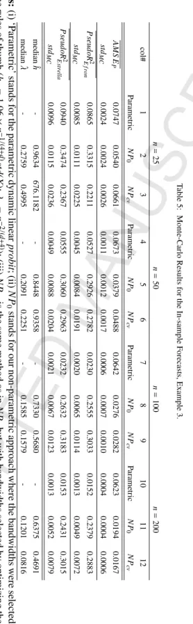
Table 5: Monte-Carlo Results for the In-sample Forecasts, Example 3. n = 25 n = 50 n = 100 n = 200 col# 1 2 3 4 5 6 7 8 9 10 11 12 Parametric N P 0 N P cv Parametric N P 0 N P cv Parametric N P 0 N P cv Parametric N P 0 N P cv A M S E P 0.0747 0.0540 0.0661 0.0673 0.0379 0.0488 0.0642 0.0276 0.0282 0.0623 0.0194 0.0167 st d M C 0.0024 0.0024 0.0026 0.0011 0.0012 0.0017 0.0006 0.0007 0.0010 0.0004 0.0004 0.0006 P seud oR 2 E fr on 0.0865 0.3315 0.2211 0.0527 0.2926 0.2782 0.0230 0.2555 0.3033 0.0152 0.2379 0.2883 st d M C 0.0085 0.0111 0.0225 0.0045 0.0084 0.0191 0.0020 0.0065 0.0114 0.0013 0.0049 0.0072 P seud oR 2 E st rel la 0.0940 0.3474 0.2367 0.0555 0.3060 0.2963 0.0232 0.2632 0.3183 0.0153 0.2431 0.3015 st d M C 0.0096 0.0115 0.0236 0.0049 0.0088 0.0204 0.0021 0.0067 0.0123 0.0013 0.0052 0.0079 median ˆ h -0.9634 676.1182 -0.8448 0.9358 -0.7330 0.5680 -0.6375 0.4691 median ˆ λ -0.2759 0.4995 -0.2091 0.2251 -0.1585 0.1579 -0.1201 0.0816 Notes: (i) ‘P arametric’ stands for the parametric dynamic linear pr obit ;(ii) N P 0 stands for our non-parametric approach where the bandwidths were selected via the rules of thumb ( h 0 = 1 . 06 × n − 1 / (4 + d ) st d ( X ); λ 0 = n − 2 / ( d + 4) ); (iii) N P cv is the same method as in N P 0 but with bandwidths selected by optimizing the (lea ve-one-out) CV in each replication;
Table 6: Monte-Carlo Results for the Out-of-sample Forecasts, Example 3. n = 25 n = 50 n = 100 n = 200 col# 1 2 3 4 5 6 7 8 9 10 11 12 Parametric N P0 N P0 / 1 . 1 Parametric N P0 N P0 / 1 . 1 Parametric N P0 N P0 / 1 . 1 Parametric N P0 N P0 / 1 . 1 A M S EP (1-ahead) 0.0999 0.0877 0.0895 0.0752 0.0485 0.0470 0.0672 0.0315 0.0293 0.0621 0.0202 0.0183 st dM C 0.0047 0.0054 0.0057 0.0027 0.0028 0.0029 0.0020 0.0015 0.0014 0.0018 0.0009 0.0008 A M S EP (2-ahead) 0.0554 0.0547 0.0561 0.0384 0.0293 0.0289 0.0338 0.0204 0.0196 0.0302 0.0134 0.0124 st dM C 0.0036 0.0049 0.0050 0.0015 0.0015 0.0016 0.0012 0.0011 0.0011 0.0010 0.0007 0.0006 median ˆh -0.9634 0.8759 -0.8448 0.7680 -0.7330 0.6664 -0.6375 0.5796 median ˆλ -0.2759 0.2509 -0.2091 0.1901 -0.1585 0.1441 -0.1201 0.1092 Notes: (i) ‘P arametric’ stands for the parametric dynamic linear pr obit ;(ii) N P0 stands for our non-parametric approach where the bandwidths were selected via the rule-of-thumb ( h0 = 1 . 06 × n − 1 / (4 + d ) st d ( X ); λ0 = n − 2 / ( d + 4) ); (iii) N P0 / 1 . 1 is the same method as in N P0 but with the rule-of-thumb bandwidths di vided by 1.1;
References
Aitchison, J., Aitken, C. G. G., 1976. Multivariate binary discrimination by the kernel method. Biometrika 63 (3), 413–420.
Bierens, H. J., 1983. Uniform consistency of kernel estimators of a regression function under generalized conditions. Journal of the American Statistical Association 77, 699–707.
Chauvet, M., Potter, S., 2005. Forecasting recessions using the yield curve. Journal of Forecasting 24 (2), 77–103.
Cosslett, S., 1987. Efficiency bounds for distribution-free estimators of the binary choice and the censored regression models. Econometrica 55 (3),
559–585.
Cosslett, S. R., 1983. Distribution-free maximum likelihood estimator of the binary choice model. Econometrica 51 (3), 765–782. de Jong, R. M., Woutersen, T., 2011. Dynamic time series binary choice. Econometric Theory 27, 673–702.
Dong, Y., Lewbel, A., 2011. Nonparametric identification of a binary random factor in cross section data. Journal of Econometrics 163 (2), 163–171. Dueker, M., 1997. Strengthening the case for the yield curve as a predictor of U.S. recessions. Review - Federal Reserve Bank of St. Louis 79 (2),
41–51.
Dueker, M., 2005. Dynamic forecasts of qualitative variables: A qual var model of U.S. recessions. Journal of Business and Economic Statistics 23 (1), 96–104.
Efron, B., 1979. Bootstrap methods: Another look at the jackknife. The Annals of Statistics 7 (1), 1–26.
Estrella, A., 1998. A new measure of fit for equations with dichotomous dependent variables. Journal of Business and Economic Statistics 16 (2), 198–205.
Estrella, A., Mishkin, F., 1998. Predicting U.S. recessions: Financial variables as leading indicators. The Review of Economics and Statistics 80 (1), 45–61.
Estrella, A., Mishkin, F. S., 1995. Predicting U.S. recessions: Financial variables as leading indicators, working Paper 5379, National Bureau of Economic Research.
Fan, J., Heckman, N. E., Wand, M. P., 1995. Local polynomial kernel regression for generalized linear models and quasi-likelihood functions. Journal of the American Statistical Association 90, 141–150.
Fr¨olich, M., 2006. Non-parametric regression for binary dependent variables. Econometrics Journal 9, 511540.
Hall, P., Johnstone, I., 1992. Empirical functionals and efficient smoothing parameter selection (with discussion). Journal of Royal Statistical
Society, Series B 54, 475–530.
Hall, P., Li, Q., Racine, J., 2007. Nonparametric estimation of regression functions in the presence of irrelevant regressors. The Review of Eco-nomics and Statistics 89 (4), 784789.
Hall, P., Marron, J. S., 1991. Local minima in crossvalidation functions. Journal of Royal Statistical Society, Series B 53, 245252.
Harding, D., Pagan, A., 2011. An econometric analysis of some models for constructed binary time series. Journal of Business and Economic Statistics 29 (1), 86–95.
H¨ardle, W., Hall, P., Marron, J. S., 1988. How far are automatically chosen regression smoothing parameters from their optimum? Journal of American Statistical Association 83, 86–101.
Honore, B., Lewbel, A., 2002. Semiparametric binary choice panel data models without strictly exogeneous regressors. Econometrica 70 (5), 2053–2063.
Horowitz, J. L., 1992. A smoothed maximum score estimator for the binary response model. Econometrica 60 (3), 505–531.
Hu, L., Phillips, P. C. B., 2004. Dynamics of the federal funds target rate: a nonstationary discrete choice approach. Journal of Applied Econometrics 19 (7), 851–867.
Kauppi, H., 2012. Predicting the direction of the fed’s target rate. Journal of Forecasting 31 (1), 47–67.
Kauppi, H., Saikkonen, P., 2008. Predicting U.S. Recessions with Dynamic Binary Response Models. Review of Economics and Statistics 90 (4), 777–791.
Klein, R. W., Spady, R. H., 1993. An efficient semiparametric estimator for binary response models. Econometrica 61 (2), 387–421.
Lewbel, A., 2000. Semiparametric qualitative response model estimation with unknown heteroscedasticity or instrumental variables. Journal of Econometrics 97, 145–177.
Li, D., Simar, L., Zelenyuk, V., 2016. Generalized nonparametric smoothing with mixed discrete and continuous data. Computational Statistics & Data Analysis 100, 424–444.
Li, Q., Racine, J., 2007. Nonparametric Econometrics: Theory and Practice. Princeton University Press.
Manski, C., 1975. Maximum score estimation of the stochastic utility model of choice. Journal of Econometrics 3 (3), 205–228.
Manski, C., 1985. Semiparametric analysis of discrete response: Asymptotic properties of the maximum score estimator. Journal of Econometrics 27 (3), 313–333.
Masry, E., 1996. Multivariate local polynomial regression for times series: uniform strong consistency and rates. Journal of Times Series Analysis 17, 571–599.
Matzkin, R., 1992. Nonparametric and distribution-free estimation of the binary threshold crossing and the binary choice models. Econometrica 60, 239–270.
Matzkin, R. L., 1993. Nonparametric identification and estimation of polychotomous choice models. Journal of Econometrics 58, 137–168. McFadden, D., 1973. Frontiers of Econometrics. New York: Academic Press, Ch. Conditional logit analysis of qualitative choice behavior. McFadden, D., 1974. The measurement of urban travel demand. Journal of Public Economics 3 (4), 303–328.
Moysiadis, T., Fokianos, K., 2014. On binary and categorical time series models with feedback. Journal of Multivariate Analysis 131, 209–228. Park, B., Marron, J., 1990. Comparison of data-driven bandwidth selectors. Journal of the American Statistical Association 85, 66–72. Park, J. Y., Phillips, P. C. B., 2000. Nonstationary binary choice. Econometrica 68 (5), 1249–1280.
Racine, J. S., Li, Q., 2004. Nonparametric estimation of regression functions with both categorical and continuous data. Journal of Econometrics 119, 99–130.