Comparative Study of Dimension Reduction Approaches With Respect to Visualization in 3-Dimensional Space

(1)

Kennesaw State University

DigitalCommons@Kennesaw State University

Master of Science in Computer Science Theses Department of Computer Science

Spring 5-6-2016

Comparative Study of Dimension Reduction

Approaches With Respect to Visualization in

3-Dimensional Space

Pooja Chenna

Follow this and additional works at:http://digitalcommons.kennesaw.edu/cs_etd

Part of theOther Computer Engineering Commons

This Thesis is brought to you for free and open access by the Department of Computer Science at DigitalCommons@Kennesaw State University. It has been accepted for inclusion in Master of Science in Computer Science Theses by an authorized administrator of DigitalCommons@Kennesaw State University. For more information, please [email protected].

Recommended Citation

Chenna, Pooja, "Comparative Study of Dimension Reduction Approaches With Respect to Visualization in 3-Dimensional Space" (2016).Master of Science in Computer Science Theses.Paper 3.

(2)

Comparative Study of Dimension Reduction Approaches with

Respect to Visualization on 3-Dimensional Space

Master's Thesis

By

Pooja Chenna

MSCS Student

Department of Computer Science

Kennesaw State University, USA

Submitted in partial fulfillment of the

Requirements for the degree of

Master of Science in Computer Science

(3)

(4)

DEDICATION

This thesis is dedicated to my family,

(5)

ACKNOWLEDGEMENTS

I would like to thank Dr. Ying Xie for his support, encouragement and

motivation through this entire process.

I am very thankful for this experience.

I would also like to thank my thesis committee members, Dr. Shi, and Dr. He

for their insightful comments and valuable suggestions.

This research paper is made possible through the help and support from

everyone, including my professors, parents, my husband, family and friends.

(6)

LIST OF TABLES

Table 1: Attribute information for breast cancer dataset ... 13

Table 2: Comparison between RBMs and autoencoders ... 24

Table 3: Categorization of dimension reduction techniques ... 25

Table 4:COMPARISON OF RELATED WORK ... 28

Table 5: Step-by-Step procedure for reduction and evaluation ... 30

Table 6: Difference between normalization and standardization ... 31

Table 7: Two forms of min-max normalization ... 32

Table 8: Scala Statements for running k-means ... 33

Table 9: Scala statements to run k-means with best chosen ‘k’ ... 35

Table 10: Dummy dataset details for entropy calculation illustration ... 37

Table 11: Datasets and relevant information ... 47

Table 12: Entropy values for Ionosphere dataset ... 50

Table 13: Entropy values for breast cancer dataset ... 51

Table 14: Attribute information for wine dataset ... 52

Table 15: Entropy values for wine dataset ... 54

Table 16: Attribute information for shuttle landing control dataset ... 55

Table 17: Entropy values for shuttle landing dataset ... 57

Table 18: Attribute information for ecoli dataset ... 58

Table 19: Entropy values for ecoli dataset ... 60

(7)

LIST OF FIGURES

Figure 1: Parallel co-ordinate display for n-dimensional dataset ... 11

Figure 2: Two scatter plots of random datasets in 3-D space ... 12

Figure 3: Snapshot for breast cancer dataset... 14

Figure 4: 3D scatter plot for breast cancer dataset with PCA ... 15

Figure 5: New data with unknown classes (in black circles) in breast cancer dataset... 15

Figure 6: Restricted Boltzmann Machine ... 22

Figure 7: Deep Belief Network ... 23

Figure 8: Algorithm for k-means ... 33

Figure 9: Clustering Score for random dataset ... 34

Figure 10: Graph for clustering score and wide range of k ... 35

Figure 11: Clustering for dummy dataset ... 38

Figure 12: Clustering for dummy dataset after reduction ... 38

Figure 13: Entropy Calculation Results in ECL ... 40

Figure 14: ECL Results for SVD for random dataset ... 42

Figure 15: ECL results for PCA for random dataset... 43

Figure 16: ECL results for DBN for random dataset ... 44

Figure 17: Network architecture for DBN ... 44

Figure 18: ECL results for stacked auto-encoders for random dataset ... 45

Figure 19: Network architecture for Stacked Auto-encoders ... 46

Figure 20: Snapshot of Ionosphere Dataset ... 48

Figure 21: Clustering Score and its graph for Ionosphere dataset ... 48

(8)

Figure 23: Clustering Score and its graph for Breast Cancer dataset ... 50

Figure 24: Visualizations for reduced breast cancer 3-dimensional dataset ... 51

Figure 25: Snapshot of normalized wine dataset ... 53

Figure 26: Clustering Scores and its graph for wine dataset ... 53

Figure 27: Visualizations for reduced wine 3-dimensional data ... 54

Figure 28: Snapshot of shuttle landing control dataset ... 55

Figure 29: Clustering scores and its graph for shuttle dataset ... 56

Figure 30: Visualizations for shuttle landing control reduced 3-dimensional dataset ... 57

Figure 31: Snapshot for ecoli dataset ... 59

Figure 32: Clustering Scores and its graph for ecoli dataset ... 59

Figure 33: Visualizations for ecoli reduced 3-dimensional dataset ... 60

Figure 34: HPCC Machine Learning Hierarchy ... 63

Figure 35: HPCC Architecture... 64

Figure 36: ECL IDE and ECL Watch ... 65

Figure 37: Parameters for DBN ... 70

Figure 38: Code Snippet ... 70

Figure 39: Code Snippet ... 71

Figure 40: Movie-Ratings dataset ... 72

Figure 41: Parameters used for Movie-Ratings dataset ... 72

Figure 42: Test data for movie-ratings ... 72

Figure 43: Learnt Model ... 73

(9)

ABSTRACT

In the present big data era, there is a need to process large amounts of unlabeled data and find some patterns in the data to use it further. If data has many dimensions, it is very hard to get any insight of it. It is possible to convert high-dimensional data to low-dimensional data using different techniques, this dimension reduction is important and makes tasks such as classification, visualization, communication and storage much easier. The loss of information should be less while mapping data from high-dimensional space to low-dimensional space. Dimension reduction has been a significant problem in many fields as it needs to discard features that are unimportant and discover only the representations that are needed, hence it gathers our interest in this problem and basis of the research. We consider different techniques prevailing for dimension reduction like PCA (Principal Component Analysis), SVD (Singular Value Decomposition), DBN (Deep Belief Networks) and Stacked Auto-encoders. This thesis is intended to ultimately show which technique performs best for dimension reduction with the help of studied experiments.

(10)

CHAPTER 1 Motivation, Problem Statement and Contribution

1.1 Background

With the advent of big data, lot of research is being done on how to deal with problems coming along. Big data refers to a large amount of structured and unstructured data usually in some petabytes and makes it tough to investigate more on the data. Thus problems like querying competently, analysing, visualization etc…arouse with big data. In this paper, we deal with the problem of dimension reduction and then visualization.

The challenges that big data is facing are given in terms of 4 V’s namely “Volume”, “Velocity”, “Veracity” and “Variety” [1, 2]. In this context, dimension reduction comes into picture in dealing with one of the challenges of big data. High volume of data may result in multiple dimensions for data. It is really complex to analyze data when it has many dimensions, thus there should exist any of the dimension reduction techniques that help in reducing dimensions without losing the structure of data and it’s meaning [3].

Traditional and deep-rooted methods of dimension reduction are done using factor analysis. Principal Component Analysis and Singular Value Decomposition come under this category. But these kind of techniques are not suitable for non-linear complex data. To efficiently deal with non-linear complex data many other dimension reduction techniques are proposed today but deep learning techniques prevail among them.

1.2 Motivation

When we consider dimension reduction techniques in particular, PCA and SVD are two examples of conventional methods whereas Deep Belief Networks and Stacked Auto-encoders are two examples of deep learning techniques that can easily handle non-linear and big data. Dimension Reduction is a significant problem in many real world studies because big data always has high dimensions and mapping the data from high dimensions to low dimensions is essential to increase the efficiency of data analysis and handling [4]. Most of the machine learning techniques till now exploited linear transformation using factorization or orthogonal projections in dimension reduction. These kind of techniques usually are not effective for

(12)

non-11

linear feature transformations and but may be effective in solving many simple-data with limited constraints. Deep learning on the other hand has high representational power and deals with complex data.

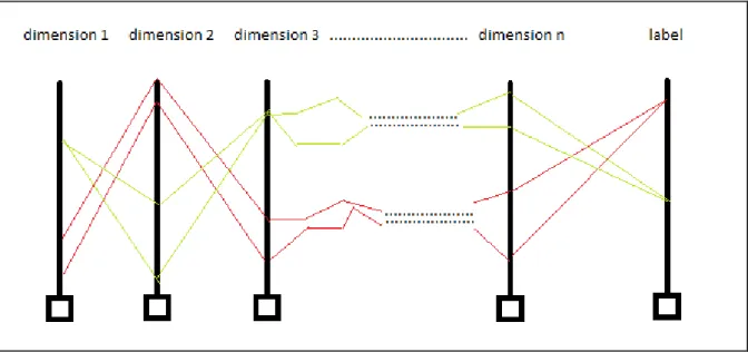
Visualization and data compression are treated as the two important motivation subjects that incited interest in us about research in dimension reduction. Visualization can be performed in two ways, keeping all the dimensions or by reducing the dimensions. Heatmap, parallel co-ordinates, line graphs, Radviz, Polyviz etc.. are some of the visualization techniques. For example, parallel co-ordinates technique use ‘n’ parallel vertical lines if there are ‘n’ dimensions where the co-ordinates vary from minimum and maximum values for nth dimension. Now a poly line (represented as red and green lines in Figure 1) is drawn connecting all the ‘n’ parallel vertical lines or axes to represent a data point [5, 6].

Figure 1: Parallel co-ordinate display for n-dimensional dataset

Figure 1 has parallel axes denoted by dimension 1, dimension 2, ……, dimension n. Green poly lines represent one type of class and red poly lines represent another type of class.

Similarly heat map uses a data grid or array of cells and color it based on the data points, line graphs use a continuous function in the form of a separate graph for each dimension. Representation and details about Radviz can be obtained from [7] and polyviz is just an extension for radviz with dimensions represented in the form of lines and not points to give more

(13)

12

insight about data distribution [8]. But all these techniques where all the dimensions are kept do not help a lot in data exploration and analysis. It is impractical to visualize the data with high dimensions, hence dimension reduction has to be performed for an intuitive visualization. There are many ways to perform dimension reduction using PCA, MDS, Isomap, LLE, neural networks, SVD etc…We choose to compare PCA, SVD and deep learning techniques in this study.

Research work in [9] clearly states about the challenges faced by big data visualization like real-time scalability, perceptual scalability and interactive scalability. Summary of all these challenges include data being large, even with visualization it is difficult for a human to extract meaningful data, limited screen availability because of which everything cannot be seen, limitation of data size or storage to visualize, complex querying may freeze or crash the visualization systems.

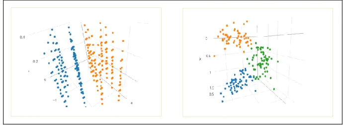
Dimension reduction is the most common step used for data reduction and extracting information from big data. Few dimension reduction techniques have the ability to remove the correlation among the data variables and few others have data divided among the clusters which simplifies the process of data analysis. Reducing the dimensions to 2 or 3 helps in improved visualization. For example, scatter plots shown in Figure 2.

Figure 2: Two scatter plots of random datasets in 3-D space

A scatterplot is a point projection of the data into 2D or 3D space and one of the most used visualization methods [8]. Visualization in 3D space shown in Figure 2 is so clear and it is

(14)

13

further easy to predict about any new data in these type of plots. This can be easily explained using an example scenario using breast cancer dataset.

Breast cancer dataset

Table 1: Attribute information for breast cancer dataset

Number of Attributes : 9 Number of classes : 2 Number of Samples : 699

Attribute Information:

1. Clump Thickness 2. Uniformity of Cell Size 3. Uniformity of Cell Shape 4. Marginal Adhesion

5. Single Epithelial Cell Size 6. Bare Nuclei

7. Bland Chromatin 8. Normal Nucleoli 9. Mitoses

Benign or Malignant – Classes

Table 1 gives the details about breast cancer dataset such as number of dimensions and number of classes it has.

(15)

14

Figure 3: Snapshot for breast cancer dataset

Figure 3 shows initial few samples from breast cancer dataset, it gives us an idea on how data looks like. Classes are labeled as 0 or 1 instead of malignant and benign to serve as input for dimension reduction technique. The breast cancer data with 9 dimensions is chosen to be reduced to 3 dimensions for better visualization with the help of Principal Component Analysis, one of the dimension reduction techniques.

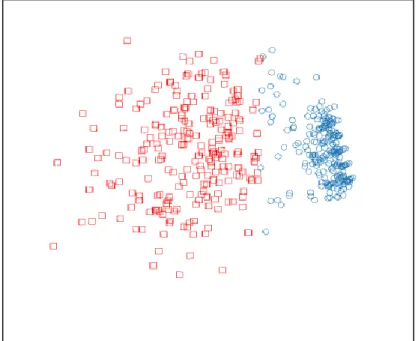
Two classes malignant and benign for breast cancer dataset are shown as blue circles and red squares in Figure 4. It is clear from Figure 4 that the two classes are easily differentiable and separable. That is the perfect advantage of visualization. Now Figure 5 talks about new data points whose class is unknown and those are shown in a different color (black).

(16)

15

Figure 4: 3D scatter plot for breast cancer dataset with PCA

Figure 5: New data with unknown classes (in black circles) in breast cancer dataset

Class labels for four samples from the original reduced dataset are made unknown for the purpose of making visual decision. The resultant dataset plot is shown in Figure 5 where the four black circles represent unknown class samples. But from the visualization in Figure 5, class can

(17)

16

be easily predicted based on examining the cluster to which this unknown class sample belongs to. This simple illustration with the help of Figure 6 makes us understand the value and benefits of visualization.

At the end, in order for an effective and intuitive visualization, data dimension reduction is considered to be an important step. At the same time, quality of dimension reduction and quality of visualization has to be ensured for efficient data analysis. So, visualization of high dimensional data preserving the original data’s intrinsic structure is the motive behind this research.

1.3 Problem Statement

Preserving the structure of data after dimension reduction plays an important role when dealing with big data. Though there are many techniques for reducing dimensions, it is necessary to check that data is reduced with minimum loss of information. If there is much loss in structure or meaning of data, the original motive of analyzing the data with lower dimensions may not be achieved properly. This work is an effort to research and propose a new approach to address this kind of problem.

During literature search, we identified a list of common limitations among past research efforts. These limitations are summarized as follows:

 Lack of thorough research that compare traditional approaches with deep learning approaches in terms of dimension reduction. In particular, most efforts are effective to compare linear techniques with non-linear techniques for dimension reduction. However, they are complete different type of research and may not be related to deep learning.

 No evidence is provided in the research about maintaining the structure and originality of data after reducing it from higher dimensions to lower dimensions. Also very few strategies are provided in order to achieve the same. In particular, there is no effort of formally specifying the methods to show that the data structure is preserved after dimension reduction.

(18)

17

Given the obtained literature search results, we define the problem statement for this thesis as follows:

This research work addresses common limitations found in past research efforts by executing an in-depth study of dimension reduction, provides visualization for high dimensional datasets while keeping the original data structure, in order to evaluate, an approach to check the information loss for original data after reducing dimensions is designed, and the proposed approach makes the comparison easier.

1.4 Research Methodology

The research methodology comprised of an intensive literature review of different articles consisting of information on big data, machine learning, deep learning, linear and non-linear dimension reduction, deep learning techniques. The research methodology involves the following activities:

1)Conduct literature search on existing comparison reviews for dimension reduction and their performance.

2)Study and analyze collected information to understand how different techniques perform on data after application and reducing dimensions.

3)Develop deep belief networks, a technique which is proposed for comparison but non-existing in HPCC deep learning module.

4)Propose an approach to check whether the loss of information is minimum for the data after dimension reduction.

5)Evaluate the proposed approach against different dimension reduction techniques for comparison.

1.5 Contribution

The objective of this thesis is to conduct an in-depth comparison of various types of dimension reduction techniques like PCA, SVD, Stacked Auto Encoders, Deep Belief Networks; study of existing methodologies for dimension reduction; develop an approach to check the information loss after reducing the dimensions; evaluate the proposed approach.

(19)

18

1) Conduct Literature Search and Develop Deep Belief Networks

i. Conduct literature search on existing deep belief network implementations in other platforms and check for their accuracy. It has to be replicated in HPCC.

ii. Conduct literature search on different linear and non-linear data dimension reduction techniques. An approach has to be determined for checking whether the structure of data is preserved.

iii. The author will compose a survey of compiled papers related to this topic and document the findings.

2) Develop an Algorithm and Approach

i. The algorithm for Deep Belief Networks is implemented and tested for accuracy.

ii. The developed algorithm is tested with the given input datasets to reduce their dimensions and visualized in a 3D space to analyze further.

iii. An approach is determined for checking the structure of data after reducing the dimensions.

3) Get Datasets

i. Suitable datasets are gathered to perform experiments.

ii. 5 datasets with more than 30 dimensions to datasets having 6 dimensions are considered for the research. Each dataset is different from its perspective. Basically they all have different characteristics, hence considered for testing.

4) Comparison Study

i. Perform simulations for all the techniques and use the unsupervised clustering, entropy determination and visualization approach for better comparison.

5) Dissemination of Results

i. Disseminate the results for ease of access and understanding. The source code will be available upon request, but this is at the discretion of the author.

(20)

19

In the next Chapter, we present literature review for all the dimension reduction techniques that are used for comparative study.

(21)

20

CHAPTER 2 Literature Review

2.1 Overview

Many research works have been done in the past to compare dimension reduction techniques [10, 11, 12, 13, 14] and other works are presented in related work section 3.2. This Chapter presents a literature review of different dimension reduction techniques and their recent applications.

2.2 Dimension reduction techniques

Upon literature review, we consider two traditional approaches and two deep learning approaches for comparison. We list below all the four approaches used for comparison in this paper.

SVD (Singular Value Decomposition):

Singular Value Decomposition is a matrix factorization method. Formally, if there is a dataset with m*n dimensions, there exists a factorization called singular value decomposition of M, of the form

M = UΣV*

where U is a unitary matrix, Σ is a diagonal matrix with non-negative real numbers on the diagonal and V is a unitary matrix. The diagonal entries of Σ are known as singular values of M.

“Singular value decomposition components of a matrix U, Σ and V can be multiplied together to recreate the original matrix exactly. However, if only a subset of rows and columns of matrices U, Σ, and V are used, then those lower-order matrices U, Σ, and V provide the best approximation of the original matrix in the least square error sense. Because of that, SVD can be seen as a method for transforming correlated variables represented by columns of the original matrix into a set of uncorrelated variables that better expose relationships that exist among the original data items. SVD can also be used as a method for identifying and ordering the dimensions along which data points exhibit the most variation.“[15]

(22)

21 PCA (Principal Component Analysis):

“Principal Component Analysis is a mathematical procedure that uses an orthogonal transformation to convert a set of observations of possibly correlated variables into a set of values of linearly uncorrelated variables called ‘principal components’. The number of principal components is less than or equal to the number of original variables. This transformation is defined in such a way that the first principal component has the largest possible variance (that is, it accounts for as much of the variability in the data as possible), and each succeeding component in turn has the highest variance possible, under the constraint that it is orthogonal (meaning uncorrelated with) to the preceding components.” [15]

DBN (Deep Belief Networks):

Deep Belief Networks is a probabilistic generative model composed of multiple layers of stochastic, hidden variables [16]. Before knowing about deep belief networks, it is important to know about Restricted Boltzmann Machines (RBMs) because RBMs are stacked to form so called Deep Belief Network. In 2006, Hinton showed that RBMs can be stacked and trained in a greedy manner to form DBNs. DBNs are graphical models which learn to extract a deep hierarchical representation of the training data.

RBMs use an algorithm called “Contrastive Divergence” instead of traditional back propagation to learn and prepare a model. The Contrastive Divergence algorithm works in two phases namely positive and negative phases. In positive phase, the input vector ‘v’ is clamped to the input layer and is propagated to hidden layer in a similar manner to feed forward neural networks and obtain a result ‘h’. In negative phase, the result ‘h’ from positive phase is propagated back to the visible layer, obtains a result v’ and the new result is again propagated to hidden layer with activation result h’.

After the positive and negative phases, weight is updated as: w(t+1) = w(t) + α(vhT – v’h’T) where α is the learning rate and w, v, v’, h, h’ are vectors.

(23)

22

Figure 6: Restricted Boltzmann Machine –Image is copied from [16]

The intuition behind the algorithm is that the positive phase reflects the network’s internal representation of the real world data. Meanwhile, the negative phase represents an attempt to recreate the data based on this internal representation. The main goal is for the generated data to be as close as possible to the real world and this is reflected in the weight update formula. In other words, the net has some perception of how the input data can be represented, so it tries to reproduce the data based on this perception. If its reproduction isn’t close enough to reality, it makes an adjustment and tries again [17].

There are different representative works using Restricted Boltzmann Machines like Deep Belief Networks, Deep Boltzmann Machines, Deep Energy Models [18]. One of the works “Deep Belief Networks” is further discussed.

Figure 7 is a representation for deep belief network. These deep belief networks are often quite powerful producing impressive results.

(24)

23

Figure 7: Deep Belief Network – Image is copied from [16]

DBNs model the joint distribution between observed vector ‘x’ and the ‘l’ hidden layers hk_as

follows:

where x = h0_{, P(h}k-1_|hk_{) is a conditional distribution for the visible units conditioned on the}

hidden units of the RBM at level k, and P(hl-1_|hl_{) is the visible-hidden joint distribution in the}

top-level RBM.

Despite these impressive characteristics of deep belief networks that suits for reducing dimensions, we also mentioned few papers in the related work – section 3.2 that explicitly discussed deep belief networks for dimension reduction.

Stacked Auto-encoders:

Stacked auto-encoders are best used for unsupervised learning as it is good in capturing hierarchical groups, that is primary layers of the network learns higher level features and as we go deeper in network, it tries to learn lower level features in deep learning that replaced the learning techniques used in conventional neural networks.

(25)

24

Stacked Auto-encoders as the name suggests is a stack of auto-encoders. They are also referred to as Stacked Auto-Associators as they try to associate the output with the input and try to find intermediate representations [19]. Traditionally, in stacked encoders output from one auto-encoder is treated as input for the next auto-auto-encoder and this process repeats till all the individual auto-encoders in the network are pre-trained [20]. The result at the output layer is with reduced dimensions. There are different variations in auto-encoder like Sparse Autoencoder, Denoising Autoencoder, Contractive Autoencoder [18]. For dimension reduction, we do not consider the attribute sparsity because the original dimensional space is reduced but not expanded.

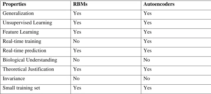
Table 2: Comparison between RBMs and autoencoders

Properties RBMs Autoencoders

Generalization Yes Yes

Unsupervised Learning Yes Yes

Feature Learning Yes Yes

Real-time training No Yes

Real-time prediction Yes Yes

Biological Understanding No No

Theoretical Justification Yes Yes

Invariance No No

Small training set Yes Yes

Table 2 is the comparison study between only two deep learning techniques restricted boltzmann machines and autoencoders. It is extracted from [18] where the comparison is performed among different other deep learning techniques also. From the comparison it is clear that deep learning techniques do not depend on invariance at all whereas the traditional techniques depend on variance and orthogonal transformations.

According to [21], research on dimension reduction has taken many sides like it can be done with projections or making use of neural networks or similar data or fractality. Our paper discusses dimension reduction from the sides of projections and neural networks. It is also stated in [21] that linear techniques like PCA have more time complexity and space complexity of o(m2), so they have designed an optimized RBM approach with dynamic hidden layers to show

(26)

25

the better results on MNIST [18] database. Our RBM approach uses fixed number of hidden layers but achieves good results after trying multiple combinations but work accomplished in [21] is optimized by using dynamic hidden layers.

Apart from dimension reduction, deep learning techniques can be used for classification purposes also which is illustrated in [19, 22]. In [22], abstraction feature of DBN is combined with back propagation strategy for classification. A slight variation of auto-encoders is used to solve the classification problem with minimal errors in [19] and performance gap is reduced when compared to DBN.

The advantages of deep learning techniques over traditional techniques are:

 It uses unsupervised training which eliminates the need of labels for training.

 Local optima can be prevented.

 Data can be separated more easily.

 Meaningful representations can be made.

Due to the growing research on non-linear dimension techniques, which necessarily need not be deep learning techniques but may be variations of PCA like Kernel PCA and others like LLE, HLLE etc…one may have the intuition that non-linear techniques are more preferred to linear techniques. But through research conducted in [23], it may be clear that it is not always non-linear techniques that prevail. For datasets with a lot of noise and lot many outliers, non-non-linear techniques are not best suitable. Table 3 gives categorization of all the dimension reduction techniques that makes linear, non-linear, traditional and deep learning terminologies clear.

Table 3: Categorization of dimension reduction techniques

Reduction Technique Type of suitable data Type of technique

PCA Linear Traditional

SVD Linear Traditional

Deep Belief Networks Linear and Non-linear Deep Learning Stacked Autoencoders Linear and Non-linear Deep Learning

(27)

26

For deep learning techniques, if there is one hidden layer and linear with certain nodes, then the projection is similar to PCA. If the hidden layers are non-linear, then there can be different kinds of abstraction which lead to better results [4].

Linearity and non-linearity mostly differ in the cost function used in respective approaches. In traditional PCA and SVD approaches, it’s just the matrix factorization involved which is linear. But in other non-linear techniques and deep learning techniques complex functions are used to deal with non-linear data.

Though it is learnt that there are many techniques for performing the task of dimension reduction, it is important to realize how to reduce the dimensions. Dimension reduction involves two important steps namely variable selection and feature extraction [24]. All the approaches discussed in this paper PCA, SVD, deep belief networks and stacked auto-encoders are feature extracting methods. They concentrate on finding the best features from given set of high dimensional space which represent the original data. It can be found based on variance if it is traditional approach or based on abstraction property if it is deep learning technique.

In the next Chapter, we introduce approach on how to check whether the structure of original data after dimension reduction is preserved.

(28)

27

CHAPTER 3 K-means Clustering based Approach, Dimension Reduction,

Visualization and Entropy Determination

3.1 Overview

This Chapter introduces the works done by different authors and strategies used for comparison in Section 3.2. Next we introduce the approach on entropy determination after finding the good ‘k’ value, reducing the dimensions and then performing the clustering of reduced data to check the entropy of which technique is low. However, the goal is to visualize high dimensional data in a 3D space intuitively while keeping the original data structure as much as possible. Thus proposed approach helps in realizing our goal. Benefits of dimension reduction and visualization are given with an example in chapter 1 under motivation. The design details and strategy used for comparison in this paper is clearly given in Section 3.3. Section 3.4 is to list out the benefits of proposed approach when compared to existing approaches and section 3.5 explains how the reduction is performed with each of the dimension reduction techniques.

3.2 Related Work

In [3], a comprehensive comparative study of 12 linear and non-linear techniques are used for dimension reduction. Testing is performed on artificial and natural datasets. Evaluation criteria used is based on generalization errors in classification tasks. K-nearest neighbor classifier is employed because of its high variance. It is believed by the authors that high variance helps in judging the structure of the data. They also chose generalization errors rather than reconstruction errors because no conclusion can be drawn when the reconstruction error is high, it may not mean that dimension reduction did not perform well. Finally based on the experiments it is concluded in the paper that in spite of high variance exhibited by non-linear techniques, they are not much better when compared to traditional PCA for many datasets that do not rely on local properties.

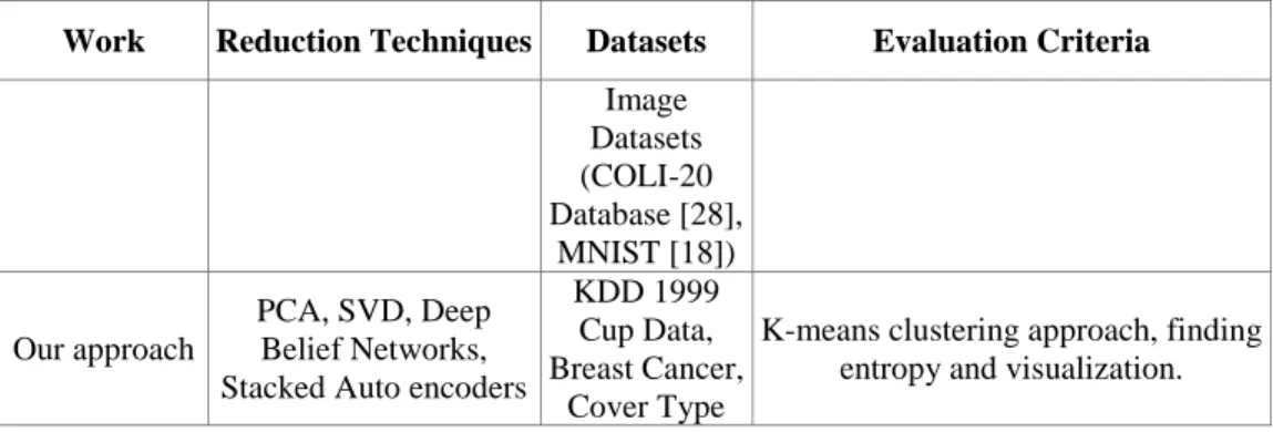
Some relevant works on dimension reduction [4, 10, 11 and 25], some related works on visualization [13, 26, 27 and 28] and many others are shown in Table 4. These works use

(29)

28

dimension reduction with different techniques. Deep Belief Networks and PCA comparison for dimension reduction with evaluation criteria being sum of squared errors difference between original one and reconstructed one is provided in [4]. A new non-linear algorithm is proposed based on eigen-value face decomposition in [10] and is compared with PCA. A non-linear generalization for PCA which uses a encoder and decoder network is used in [11], it is a neural network based dimension reduction and root mean squared error is the evaluator. Stacked auto encoders are used for dimension reduction in [25] where it is concluded that, they are not only good at reducing but also in finding repeated structures. Again a new non-linear algorithm named “Distinguishing Variance Embedding (DVE)” is designed combining the concepts of maximum variance unfolding and Laplacian Eigenmaps in [29]. In this paper, the criteria used for preserving data structure in Laplacian Eigenmaps like sum constraint is improved with strict local preserving constraints which is achieved by maximizing global variance for constraints obtained in Laplacian Eigenmaps. In the illustration, 2-dimensional and 3-dimensional embeddings show that the original local neighborhood is preserved and also in images instance, some features are clearly distinguished.

In few of the works where visualization itself is used for evaluation, it is difficult to verify the quality of visualization. A new metric based on pairwise correlation of the geodesic distance is proposed in [23]. In order to prove that the proposed metric performs better on many dimension reduction techniques, they compared it with several other metrics like Euclidean distance, spearman distance etc…

Our work is mainly focused on comparing the traditional approaches with deep learning approaches for dimension reduction. We focus on visualization of every dataset after reduction and try to validate our analysis based on visualization with the help of entropy.

In contrast to earlier work, our proposed approach gives a better way to visualize and check the loss of information using entropy determination. Entropy is used in machine learning algorithms such as decision trees to find the information gain, it is one of the powerful criteria to check on loss of information [30].

(30)

29

Work Reduction Techniques Datasets Evaluation Criteria

Noulas et al.

[4] Deep Belief Network

AR Face Database [17]

Difference between sum of squared errors of original and reconstructed

one Gering [10] Eigen Value Face

Decomposition Random Faces Reconstruction Accuracy

Teli [11] Neural Network (Encoder – Decoder)

MNIST [18], USPS, Olivetti

Face Dataset [19]

Root Mean Square Error

Maaten et al. [12]

PCA, Isomap, MVU, Kernel PCA, Diffusion

Maps, Autoencoders, LLE, Laplacian Eigen

maps, Hessian LLE, LTSA, LLC, Manifold

Charting

Artificial and Natural Datasets

K-nearest neighbor generalization error

Tsai [13]

PCA, MDS, LSA, Isomap, LLE, HLLE, LTSA

Blog Entries Visualization and finding outliers

Claveria et.al .[14] CATPCA (categorical PCA), MDS Tourist Destinations (categorical data)

Trending tourism is analysed in top 10 world destinations which is shown

graphically Wang et al. [25] Stacked Auto-encoders Synthesized Data, MNIST [18], Olivetti Face Dataset [19] Visualization Venna et.al. [26] PCA, MDS, LLE, Laplacian Eigenmap, HLLE, Isomap, CCA, CDA, maximum variance unfolding, LMVU, local MDS Plain s-curve dataset, noisy s-curve dataset, mouse gene expression, gene expression compendium, sea-water temperature time series

Neighborhood Retrieval Visualizer

Najim et.al. [27]

PCA, CCA, CDA, Trustworthy Stochastic Proximity Embedding and 17 other linear and non-linear methods Synthetic data (curved cylinder), Tensor colored image dataset

Quality of visualization using residual variance, correlation function and local continuity

Dzwinel et.al. [28]

nr-MDS (variant of MDS)

MNIST [18],

Reuters Interactive Visualization

Wang et al. [29] Distinguishing Variance Embedding Synthetic Data (helix, Swiss roll, Punctured Sphere, Twin Peaks, Gaussian) and

Strict local distance-preserving constraints

(31)

30

Work Reduction Techniques Datasets Evaluation Criteria

Image Datasets (COLI-20 Database [28], MNIST [18]) Our approach PCA, SVD, Deep Belief Networks, Stacked Auto encoders

KDD 1999 Cup Data, Breast Cancer,

Cover Type

K-means clustering approach, finding entropy and visualization.

3.3 Unsupervised Approach for Evaluating Performance of Dimension Reduction With Respect To Visualization

Ideally, we can take the original dataset with any number of dimensions, use any of the dimension reduction techniques to make it low dimensional data and then visualize it. But in order to visualize high-dimensional data in an intuitive way, we need to reduce the dimensions to three but at the same time ensure that whether reduced data is having same structure as the original data, for which we use entropy to evaluate. This approach involves unsupervised k-means approach to group the data and evaluation using entropy determination, then comparison is performed. A step wise approach is shown in the Table 5.

Table 5: Step-by-Step procedure for reduction and evaluation

Step 1.Examine the data, preprocess the data if required Step 2. Run k-means on it with wide range of k-values. Step 3.Determine the suitable k-value for the dataset.

Step 4.Discard the original labels and assign cluster numbers as labels for all the samples. Step 5. Perform dimension reduction for original data.

Step 6.Visualize the data in 3D space.

Step 7.Using the new cluster labels, find the entropy for the reduced data to evaluate and to compare.

The value of entropy in Step 7 of Table 5 talks about the amount of loss of information, if the entropy is low then the loss is less. Thus entropy can be used as a measure to evaluate the quality of clustering [31] and also dimension reduction.

(32)

31

Our idea is to find the entropy values of reduced dataset by repeating the procedure explained in Table 5 for different dimension reduction techniques and then compare the entropy score. The lowest entropy score recorded for the dataset with the reduction technique used is chosen as the best approach for dimension reduction. It may again vary on type of data, sparsity, relations among data etc…This evaluation and result discussion is clearly stated with the help of experimental study in chapter 4 and detailed step-by-step explanation is provided in this section.

Step 1.Examine the data, preprocess the data if required.

It is not possible to have real time data within a specific range. Real time data usually falls under a large range and also there may be possibility of categorical values. In order not to give weightage for any specific attribute while using classification or clustering algorithms or in neural networks, preprocessing the data acts as an important step. Preprocessing may involve steps like normalization or standardization. Table 6 explains major differences between normalization and standardization.

Table 6: Difference between normalization and standardization

Normalization Standardization

Used when maximum and minimum values of the dataset are known.

Used when maximum and minimum values of the dataset are unknown.

Standard deviation and variance are not involved.

Standard deviation and variance are involved.

Data after normalization is bounded within a range [32].

Data after standardization may not be completely bounded.

We use normalization for preprocessing the data for all the studied experiments since keeping data in a specific range is very important for all the algorithms used in comparative study. Normalization is specifically important before clustering because if there is a large variation among the values of attributes, one attribute may dominate over the other, hence the motive is to

(33)

32

balance all the attributes without giving weightage to any attribute in specific [40]. It is completely user’s choice to decide on which kind of normalization technique or rule has to be applied for specific dataset [33].

The kind of normalization chosen for this study is called min-max normalization. Using min-max normalization ensures data is in the range of 0 to 1. There are two min-max normalization forms again which are stated as in Table 7.

Table 7: Two forms of min-max normalization

Min-max normalization form 1 [32] (X-Xmin)/(Xmax-Xmin)

Min-max normalization form 2 [34] [(X-Xmin)/(Xmax-Xmin)]*(newXmax

-newXmin)+newXmin

In Table 7,

‘X’ refers to the data point

Xmax refers to the maximum value of X Xmin refers to the minimum value of X

newXmax refers to maximum value of the interval range in which X has to be newXmin refers to minimum value of the interval range in which X has to be

Techniques used for normalization will transform the original data but it should be confirmed that no noise is introduced in the original data [34]. Data transformation is usually linear in normalization approaches. More about normalization forms used for different datasets is presented in chapter 4.

Step 2.Run k-means on it with wide range of k-values.

The concept of k-means can be simply stated as “Use the data to move the centers” and “Use the centers to move the data” [35]. K-means is used for data that do not have labels and is a kind of unsupervised approach. It clusters the data based on the algorithm. ‘k’ in k-means refers to the number of clusters. Algorithm taken from [36] shown in Figure 8 clearly explains the basic concept of k-means clustering approach.

(34)

33

Figure 8: Algorithm for k-means [36]

The process of k-means is performed through a set of scala statements for the purpose of this study as scala has better options for machine learning library. Scala statements used for running k-means is shown in Table 8.

Table 8: Scala Statements for running k-means

def distance(a: Vector, b: Vector) = math.sqrt(a.toArray.zip(b.toArray). map(p=>p._1-p._2).map(d=>d*d).sum)

def distToCentroid(datum: Vector, model: KMeansModel) = { val cluster = model.predict(datum)

val centroid = model.clusterCenters(cluster) distance(centroid, datum)

}

import org.apache.spark.rdd._

import org.apache.spark.mllib.clustering._

def clusteringScore(data: RDD[Vector], k:Int) = { val kmeans = new KMeans()

kmeans.setK(k) kmeans.setRuns(10) kmeans.setEpsilon(1.0e-6) val model = kmeans.run(data)

data.map(datum=>distToCentroid(datum, model)).mean() }

(35)

34

In Table 8,

distance – function to calculate distance between two points

distToCentroid – function to calculate distance between data point and centroid

clusteringScore – function that helps in choosing the best ‘k’ value based on the clustering score. It sets ‘k’ value, sets the epsilon value that controls the movement of centroid in a cluster and also runs kmeans for 10 times to get a model.

data – input dataset in form of Vector.

Last statement in Table 8 prints the clustering score for a wide range of values specified based on step size (in this example, series goes like 1, 2, 3, 4,….., 11, 12 as step size is 1 and range specified is 1 to 12).

Figure 9 gives an idea of output for last scala statement (clustering score for wide range of ‘k’ values) in Table 8.

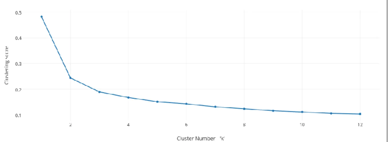
Figure 9: Clustering Score for random dataset

Now since we have clustering score for wide range of ‘k’, next step is to choose best ‘k’. It is very important to choose the best ‘k’ as it decides the best clustering.

Step 3.Determine the suitable k-value for the dataset.

One basic idea to choose the best ‘k’ is by observing the sharp change in clustering score. An easy way to determine the elbow or the sharp decrease is by plotting a graph. The elbow technique of choosing ‘k’ is taken from [31]. Figure 10 is the graph plotted for the data in Figure 9.

(36)

35

Figure 10: Graph for clustering score and wide range of k

From the Figure 10, a sharp decrease is observed at k-value ‘2’. So the best k-value is chosen to be ‘2’ for some random dataset that has clustering scores for wide range of ‘k’ as shown in Figure 9.

Step 4.Discard the original labels and assign cluster numbers as labels for all the samples.

After choosing the best ‘k’ value, k-means algorithm has to be run again on the original dataset with best ‘k’ chosen and same parameters that are used for choosing ‘k’.

Again a set of scala statements are used to run the k-means algorithm on the original dataset and predict the new clusters for the given data. Table 9 gives a piece of scala code to run k-means algorithm individually.

Table 9: Scala statements to run k-means with best chosen ‘k’

import org.apache.spark.mllib.clustering._ val kmeans = new KMeans()

kmeans.setK(2) kmeans.setRuns(10) kmeans.setEpsilon(1.0e-6) val model = kmeans.run(data) val sample = data.map(datum =>

model.predict(datum) + "," + datum.toArray.mkString(",") )

(37)

36

sample.saveAsTextFile("/user/pchenna/clustered_data”)

Code in Table 9 is not much different from code represented by using clusteringScore function in Table 8. Earlier, function is called multiple times for different values of ‘k’ but here k-means run for the best chosen ‘k’ (in this case k=2 as per step 3).

Once k-means is run with all the parameters set, model obtained is used to predict the cluster number for each sample in the original dataset. At this point, we believe that good clustering is performed with best determined ‘k’. In other words, all the homogenous samples are grouped together. So, we choose to deal with cluster numbers as labels rather than the original labels in further process. Hence as a last thing in Step 4, original labels are discarded and cluster numbers (cluster to which sample belongs to) are assigned as labels to all the samples in the original data.

“model.predict(datum)” in Table 9 predicts the cluster to which the sample belongs to, based on k-means model. After prediction, data with new cluster labels is saved in a folder called “clustered_data” from where it can be retrieved.

Step 5.Perform dimension reduction for original data.

In this step, original data dimensions are reduced to 3 using different reduction techniques. More about the dimension reduction techniques used and obtaining the data with reduced dimensions using each of the techniques is discussed in section 3.5.

Step 6.Visualize the data in 3D space.

In order to compare the different dimension reduction techniques, we choose visualization as a tool. Reduced dimensional data with each of the techniques is visualized in 3D space. Even after data reduction by dimension, there should not be much loss of information and structure. Thus visualization gives a better idea to the user about the intrinsic structure of data after reducing it to 3 dimensions. Benefits of visualization are already discussed in chapter 1.

(38)

37

Though visualization gives us better idea about the structure of the data when realized in 3D space, yet it is sometimes difficult to compare different visualizations. There has to be a way using which closer visualization for data can be differentiated. We have found that entropy as a measure which does its best job in this aspect. Further details in this Step speak about the calculation of entropy and how entropy is used to compare the quality of dimension reduction.

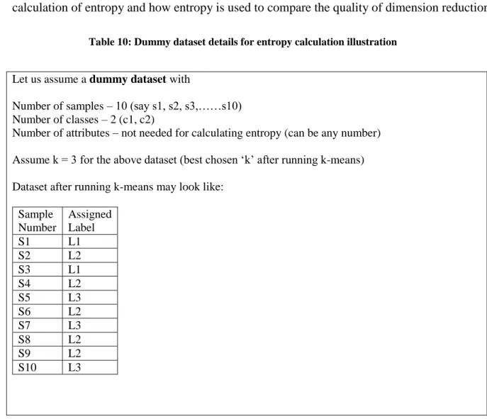
Table 10: Dummy dataset details for entropy calculation illustration

Let us assume a dummy dataset with

Number of samples – 10 (say s1, s2, s3,……s10) Number of classes – 2 (c1, c2)

Number of attributes – not needed for calculating entropy (can be any number) Assume k = 3 for the above dataset (best chosen ‘k’ after running k-means) Dataset after running k-means may look like:

Sample Number Assigned Label S1 L1 S2 L2 S3 L1 S4 L2 S5 L3 S6 L2 S7 L3 S8 L2 S9 L2 S10 L3

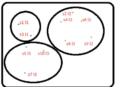
As shown in the Table 10, dataset is assumed to have 10 samples or records. Each sample may have ‘n’ attributes where ‘n’ is unknown (not required for this illustration). Originally dataset had 2 labels (or classes) but after running k-means for wide range of ‘k’, it is determined that k=3 is good for the given dataset (this is assumed as it is dummy dataset). Dataset table in Table 10 is how the samples are assigned to three clusters after running k-means algorithm. Figure 11 shows the clustered samples.

(39)

38

Figure 11: Clustering for dummy dataset

It is clearly seen from Figure 11 that there are 3 clusters with each cluster containing homogenous samples. Now Figure 12 shows the clustering result after performing the reduction (using any reduction technique).

Figure 12: Clustering for dummy dataset after reduction

It is again clear from Figure 12 that there are 3 clusters but this time clusters do not contain homogenous samples. It is bit different from the original result. Hence we use weighted cluster entropy to check how the data structure is preserved.

(40)

39

Equation 1: Individual Cluster Entropy Formula

In Equation 1,

P(S, j) refers to proportion of instances in cluster ‘S’ that belong to class label ‘j’ C refers to number of class labels

Entropy in Equation 1 is the individual entropy for each cluster. Aggregate entropy or final entropy for the data after reduction is calculated using the formula given in Equation 2.

Equation 2: Aggregate or Final Entropy Formula

In Equation 2,

|C| refers to number of samples in all the clusters |Cj| refers to number of samples in cluster Cj L refers to number of clusters

(41)

40

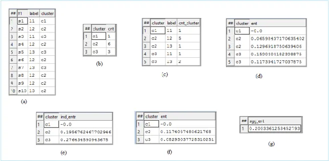
Figure 13: Entropy Calculation Results in ECL

Figure 13 shows the results obtained for calculating entropy using ECL.

Figure 13(a) is the input dataset with 10 samples. There are 3 labels (l1, l2, l3) and 3 clusters (c1, c2, c3).

Figure 13(b) is the count of number of samples in each of the 3 clusters.

Figure 13(c) is the count of samples with some label ‘l’ that belong to some cluster ‘c’. There is one sample labeled ‘l1’ in cluster ‘c1’, five samples labeled ‘l2’ in cluster ‘c2’, one sample labeled ‘l3’ in cluster ‘c2’ etc…

Figure 13(d) is the intermediate result in calculating individual entropy for each cluster. Figure 13(e) shows individual entropy for each cluster.

Figure 13(f) is the intermediate result in calculating aggregate entropy. Figure 13(g) is the final entropy or aggregate entropy.

Value of entropy always measure between 0 to 1. If entropy is low, it means that the amount of information loss is less and structure of the data is preserved. But if the entropy is high, it means that the data structure is not preserved after dimension reduction. When all the clusters contain homogenous data, entropy is ‘0’.

(42)

41 3.4 Proposed Approach Vs Existing Approach

From related work in Table 4, it is clear that many of the research works use reconstruction as a step to evaluate the structure of data after dimension reduction. After reconstructing or approximating the reduced data to original dimensions, error is computed which can be reconstruction error or root mean squared error or reconstruction accuracy. But as stated in [12], reconstruction error may not always suitable for checking the local structure of the data. Higher reconstruction error may not result in poor dimension reduction always.

Every technique has its own algorithm to reconstruct the reduced data to original data. For instance, if PCA is considered, say ‘Z’ is the reduced data, then approximated original data say ‘X’ is given by the matrix product of Ureduce and Z. The time complexity for calculating the

approximate matrix or reconstructed matrix is same as the original algorithm. If stacked auto-encoder is taken as another instance, during reduction process, the network learns its representation in an encoded form by compressing the data and extracting only the important features required. But during expansion process or reconstruction, decoding is performed which is again repeating the whole algorithm. In real-time, network architecture is usually deep which means encoding and decoding process takes a lot of time and practically infeasible. Hence this process of encoder-decoder is performed for auto-encoders because they may not have deep architectures but for stacked auto-encoders, it is really a complex process to repeat the same and even if we refer to the evaluation in [25], it is just visual comparison. Similarly reconstruction process is a tedious process in other approaches also like SVD and Deep Belief Networks. But the evaluation cannot be performed by just reconstruction, squared error difference is calculated between the original data and the reconstructed data which is treated as a measure for comparison. So, this kind of evaluation involves many steps and may take longer time in case of real-world big datasets.

In the proposed approach, we use k-means algorithm to check the clustering before and after reduction and use the cluster labels for calculating the entropy. Running k-means is scalable and easy even for big data. In real-world datasets, we do not have original labels which means unsupervised methods are essential for analysing such data sets. K-means is one of the best unsupervised approaches which helps in finding the similar data and it is reasonably fast except

(43)

42

in its worst case. Key part in k-means algorithm is choosing ‘k’ which plays a significant role. A method to choose ‘k’ is also given in the proposed approach.

Thus, we choose unsupervised clustering based approach to evaluate structure of the data after reduction rather than complex process of reconstruction.

3.5 Dimension Reduction Approaches for Comparative Study With Respect To Visualization

SVD (Singular Value Decomposition):

As mentioned in chapter 2, in order to reduce the dimensions for the original data, we need to take the subset of rows and columns of U, Σ and V to get the lower order matrices.

If we need to reduce the data from ‘n’ dimensions to 3 dimensions, then Uprime = Use only initial 3 columns for U and

Σprime = Use only 3 values for Σ

Now the lower order matrix or 3-dimensional data for the original data is given by Uprime* Σprime

Figure 14 takes an example of some random data with two dimensions and it is reduced to one dimension using SVD.

Figure 14: ECL Results for SVD for random dataset

Figure 14 (a) - matrix representation for input data with 2 dimensions Figure 14 (b) - input dataset with two dimensions in ECL output form

(44)

43

Figure 14 (d) - diagonal matrix Σ in singular value decomposition factorization Figure 14 (e) - unitary matrix V in singular value decomposition factorization Figure 14 (f) - unitary matrix Uprime, lowered from U considering only first column

Figure 14 (g) - diagonal matrix Σprime, lowered from Σ considering only one value

Figure 14 (h) - Product of Uprime and Σprime that gives the reduced data with one dimension

Figure 14 (i) - Matrix representation for Figure 14 (h)

PCA (Principal Component Analysis):

Again little introduction to PCA is already given in chapter 2. But here, description is given on how to reduce the data to 3 dimensions.

We need to consider initial 3 principal components from the ‘n’ principal components that are obtained after running PCA for the original dataset. The reduced principal components or subset of principal components is represented as “Ureduce”. Now the reduced dataset is given by the

product of original matrix with Ureduce which is X * Ureduce.

Here X has dimensions as number_of_samples * number_of_dimensions and product of X and Ureduce is 3-dimensional in our scenario.

Figure 15 takes an example of some random data with two dimensions and it is reduced to one dimension using PCA.

Figure 15: ECL results for PCA for random dataset

Figure 15 (a) - input dataset with two dimensions in ECL output form Figure 15 (b) - two principal components for the two dimensional dataset

Figure 15 (c) - one principal component which is Ureduce (reduced form of Figure 15 (b))

(45)

44 DBN (Deep Belief Networks):

DBN is spoken technically in terms of its algorithm in chapter 5. Using the same algorithmic approach, this section explains how dimension reduction is performed.

Figure 16: ECL results for DBN for random dataset

Figure 16 (a) input dataset with four dimensions in ECL output form Figure 16 (b) parameters used and their values for executing DBN

Figure 16 (c) Learnt Model for the given input with weights and bias (complete model is not shown in the figure, only part of it is presented)

Figure 16 (d) Final output with reduced dimensions to three from original four

(46)

45

Now using Figure 16 and Figure 17, dimension reduction using DBN can be explained. The dataset used is just for illustration purposes. Hence it has less number of samples and dimensions. Thus, the architecture is shallow like 4 nodes in the input layer, 3 nodes in hidden layer and 3 nodes in output layer. For the real-time datasets it may be deeper than the architecture specified in Figure 17. The number of dimensions to which the original dataset should be reduced depends on the architecture specified. Here the architecture is 4-3-3. Thus the output from DBN is 3-dimensional whereas the input fed to it is 4-dimensional. The learning technique called contrastive divergence used in DBN, getting the final output and every other detail about how algorithm works is mentioned in chapter 5. Since the batch_size is mentioned as 2 (from Figure 16), input data is processed as 3 batches with each batch having 2 samples.

Stacked Auto-encoders:

Stacked Auto-encoders work very similar to DBN in terms of stacking but the algorithm or learning technique is different. Auto-encoders are stacked together to form stacked auto-encoders. Again dimension reduction is same, the number of dimensions to which the original dataset should be reduced depends on the architecture specified.

Figure 18: ECL results for stacked auto-encoders for random dataset

Figure 18 (a) input dataset with five dimensions in ECL output form

Figure 18 (b) parameters used and their values for executing stacked auto-encoders

Figure 18 (c) Learnt Model for the given input with weights and bias (complete model not shown in the figure, only a part of it is presented)

(47)

46

Figure 19: Network architecture for Stacked Auto-encoders

Network architecture chosen for running stacked auto-encoders is 5-4-3 for given random dataset. There is no particular rule to choose the network architecture or the number of nodes in each of the layers. For the real-time datasets, number of experiments are performed and the best parameters and network architecture is presented and same is used for comparison. Since the number of nodes in output layer is 3, the reduced data or output has 3-dimensions.

In the next chapter, real-time datasets are used for dimension reduction with all the four approaches (two traditional and two deep learning). Comparison results along with visualization are also presented in the following chapter.

(48)

47

CHAPTER 4 Experimental Study

4.1Overview

In this Chapter, we demonstrate example datasets for dimension reduction with the proposed approach discussed in Chapter 3 and using HPCC deep learning module. We evaluate the results and produce a conclusion about which dimension reduction technique is suitable and gives best results for the datasets used. Moreover, we demonstrate our approach clearly with outputs obtained at each step.

Datasets used for illustration are Ionosphere [37], Breast Cancer Wisconsin (Original) [38, 39], Wine [40, 41], Shuttle Landing Control [42] and Ecoli [43]. For each dataset, results of all four dimension reduction techniques are produced and finally comparison is performed.

Table 11 shows the number of attributes, number of classes, number of instances, normalization details for all the datasets but in further sections details are provided more clearly.

Table 11: Datasets and relevant information

Datasets Number of Dimensions Number of classes Number of instances Normalized or Original Ionosphere [37] 34 2 351 Original Breast Cancer Wisconsin (Original) [38, 39] 9 2 699 Normalized using min-max normalization form 2

Wine [40, 41] 13 3 178 Normalized using

min-max normalization form 1 Shuttle Landing Control [42] 6 2 278 Normalized using min-max normalization form 1 Ecoli [43] 7 8 336 Original

Table 11 gives an idea that datasets with different characteristics are considered and chosen for experimental study.

(49)

48 4.2Dataset 1: Ionosphere

This contains radar data collected by a system in Goose Bay, Labrador [44]. Snapshot of data is presented in Figure 20. Since the data is within a specific range [-1, 1], original data is used for reduction. Normalization is not required for such data since there are no extreme values that may have more weight over the other while running the algorithm.

Figure 20: Snapshot of Ionosphere Dataset

Since normalization is not required, our next step is to find the good value for ‘k’ by running k-means over a wide range of ‘k’ say 1 to 20, as original classes are just 2, this range would be sufficient.

(50)

49

Figure 21 (a) refers to clustering score for k-values from 1 to 20

Figure 21 (b) graph plotted for k-values and their clustering scores in Figure 21 (a)

From graph in Figure 21(b), it is observed that there is a sharp change in clustering score at k-value 2 and later the change is not clearly noticeable. Hence best ‘k’ is chosen to be ‘2’ for ionosphere dataset and clustering is performed.

Figure 22: Visualization for ionosphere reduced 3-dimensional dataset

Figure 22 (a) - visualization for PCA reduced dataset Figure 22 (b) - visualization for SVD reduced dataset Figure 22 (c) - visualization for DBN reduced dataset

Figure 22 (d) - visualization for stacked auto-encoders reduced dataset

From the visualization observations using Figure 22, there is overlapping in clustering using every technique except PCA and SVD. The visualization for PCA and SVD show two separable classes, hence the loss of information should be less in such a case when compared to others. This can be verified by entropy results in Table 12.

(51)

50

Table 12: Entropy values for Ionosphere dataset

Reduction Technique Entropy Value

PCA 0.01524692879907179

SVD 0.02091038972074466

Deep Belief Networks 0.2916949005086614 Stacked Auto Encoders 0.2906937855343454

From the results in Table 12, entropy for PCA is low and then comes SVD with little difference, hence its visualization is clear and we can see that two classes are separable. Our statement that PCA and SVD may perform better just by seeing visualization is confirmed through entropy determination.

4.3Dataset 2: Breast Cancer Wisconsin (Original)

Details about breast cancer dataset is already provided in chapter 1 (Table 1 and Figure 3). Visualization and entropy results are provided in this section, but before that best k-value has to be chosen. Figure 23 helps in choosing k-value for this dataset.

Figure 23: Clustering Score and its graph for Breast Cancer dataset

Figure 23 (a) - shows clustering scores for k-values starting from 1 to 10. Figure 23 (b) - shows graph for Figure 23 (a)