The effect of general imperfections on the buckling of cylindrical shells

THE EFFECT

OF

GENERAL IMPERFECTIONS

ON THE

BUCKLING OF

CY

LINDMCAL SHELLS

Thesis by Johann Arbocz

In

Partial

Fulfillment of the Requirement@ For

the

Degree of

Doctor

of Philosophy

California Institute of Technology Pasadena, California

1968

ii

ACKNOWLEDGMENT

The author wishes to e x p r e s s his s i n c e r e appreciation to Dr. E. E. Sechler for his guidance of the work c a r r i e d out in this investi- gation; D r .

C. D. Babcock for h i s advice and comments; M e s s r s .

Marvin J e s s e y , Clarence Hemphill and Richard Luntz for t h e i r help in setting up the experiments; M r s . Betty Wood for h e r excellent drawings and M i s s Helen Burrus for bearing with my handwriting and typing the manuscript so skillfully.

This study was supported in p a r t by the National A.eronautics and Space Administration under Research Grant NsC- 18-59 and this aid i s gratefully acknowledged.

iii

ABSTRACT

An experimental and theoretical investigation of the effect of general imperfections on the buckling load of a c i r c u l a r cylindrical shell under axial compression was c a r r i e d out.

A non-contact probe has been used to make complete i m p e r - fection surveys on electroformed copper shells before and during the loading p r o c e s s up to the buckling load. The data recording p r o c e s s has been fully automatgd and the data reduction was done on a n IBM 7094. Three-dimensional plots were obtained of the m e a s u r e d initial imperfection s u r f a c e s and of the growth of these imperfections under increasing axial load. The modal components of the m e a s u r e d i m p e r - fection s u r f a c e s were also obtained.

iv

TABLE O F CONTENTS PART

I INTRODUCTION

II

EXPERIMENTAL PROGRAM 1. T e s t Equipment

a. T r a v e r s i n g Mechanism

b. Model Control Unit

6. P i c k - u p S y s t e m

d. Data Control Unit e , Digital Voltmeter f. C a r d Punch

2 . Check-out of t h e T e s t Equipment a. Scans of Known Contours

b. Circumferential T i m e Delay Check-out c. H y s t e r e s i s and Repeatability of the

Measured Data

3 . Fabrication of the T e s t Specimen a. Wall Thickness

b. M a t e r i a l P r o p e r t i e s 4. T e s t P r o c e d u r e

a. Load Cell

b. Calibration of the Pick-up c. Installing the T e s t Shell

d. Initial Imperfection Measurements

e . Monitoring of the S t r a i n Gages

PAGE 1 3 3 3 5 6 7 8 8 8 8 10 11

v

TABLE O F CONTENTS (Contld) PART

5 . Data Reduction

-

Main P r o g r a m a. Best F i t Polynomial to Pick-up

Calibration Data

b. Definition of the "Perfect1' Cylinder c. Finding Harmonic Components of the

Measured Imperfection Surface

6 . Data Reduction

-

Auxiliary P r o g r a m s a. T h r e e

-

Dimensional P l o t s

b. Computing the Growth of Harmonic Components

7. T e s t Results 25

I11 COMPARISON WITH THEORY 30

1. Donnell' s Shell Equations 3 1

2. Nonlinear Buckling Equations 32

3. Buckling of a P e r f e c t Shell 38 4. Buckling of a Shell with Axisymrmetric 39

Imperfection

5. Buckling of a Shell with Both Axisymmetric 41 PAGE

18 19

and A s y m m e t r i c Imperfections

6.

Numerical Results

TABLE O F CONTENTS (Contld) PART

REFERENCES

APPENDIX

A TABLES FIGURES

PAGE

52

5 5

64

TABLE I I1 111

IV

v

VI VII VIII vii

LIST O F TABLES

Repeatability Checks

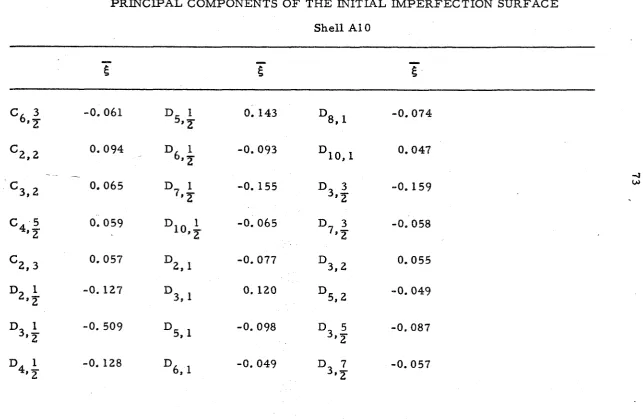
Principal Components of the Initial Imperfection

Surface

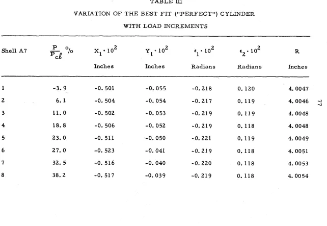
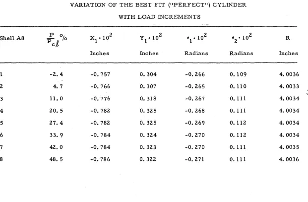
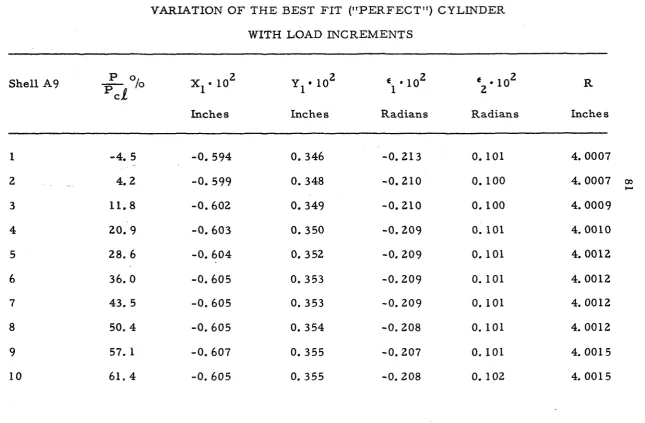
Variation of the Best Fit "Perfect" Cylinder with

Load Increments

Summary of Buckling T e s t s

Summary of llCriticalll Fourier Coefficients Summary of Wavenumbers

Numerical Results

Comparison of Theory and Experiment

PAGE

64

FIGURE 1 2 3

viii

LIST O F FIGURES

PAGE

T rave r sing Mechanism 152

P a r t i a l l y Assembled Scanning Mechanism 153 Schematic Layout of the Shell Buckling Experiment 154 Measuring Imperfections

Model Control Unit 155

Pick-up Circuit 156

M i c r o m e t e r Measurement of Known Contour 157 Compared t o Pick-up M e a s u r e m e n t s

Constant Speed T r a v e r s e of Known Contour 158 Compared to "Staticfg M i c r o m e t e r Measurement

T i m e Delay f o r Punch Control 159

Adjustment of T i m e Delay 159

H y s t e r e s i s Check 160

Testing Machine and Data Acquisition Equipment 161 Details s f Testing Machine Loading S c r e w 162

Load Cell 163

Pick-up Calibration Set Up 164

Typical Pick-up Calibration Curve 165 Cylindrical Shell Testing Configuration 166

Layered Main P r o g r a m 167

Best Fit Cylinder Reference Axis 168

Initial Imperfection, Shell A7 169

ix

LIST OF FIGURES (Contld) FIGURE

21 Initial Imperfection, Shell A9 22 Initial Imperfection, Shell A 10 23 Initial Imperfection, Shell A1 2 24 Prebuckling Deformation Growth a t

P / P c j

=

0.06 1, Shell A7

25 Prebuckling Deformation Growth at P / P c j = 0.325, Shell A7

26 Prebuckling Deformation Growth a t

p/pcL! = 0.539, Shell A7

27 Local Buckling Deformation, Shell A7 2 8 Prebuckling Deformation Growth a t

P/PcL

=

0.637, Shell A8

29 Rrebuckling Deformation Growth a t P / P c j = 0.722, Shell A9

30 Prebuckling Deformation Growth a t

P ' P c ~ = 0.439, Shell A10

3 1 Prebuckling Deformation Growth a t P / P c j = 0.594, Shell A12

32 Local Buckling Deformation, Shell A1 0 33 P o s t Buckling Deformation, Shell A7 34 P o s t Buckling Deformation, Shell A8 35 P o s t Buckling Deformation, Shell A9 36 P o s t Buckling Deformation, Shell A1 0 37 P o s t Buckling Deformation, Shell A12

FIGURE

38 39 4 0 41 42 43 44 45 46 X

LIST O F FIGURES (Cont'd)

Load Distribution Near Buckling Load Distribution Near Buckling

Growth of F o u r i e r Coefficients f o r Shell A7 Growth of F o u r i e r Coefficients f o r Shell A8 Growth of F o u r i e r Coefficients f o r Shell A9 Growth of F o u r i e r Coefficients f o r Shell A10 Growth of F o u r i e r Coefficients f o r Shell A12 Shell Geometry and Coordinate System

P o s t Buckling Equilibrium P a t h s for P e r f e c t Shells

P o s t Buckling Equilibrium P a t h s f o r Shells with Axisymmetric Imperfections

Po s t Buckling Equilibrium P a t h s f o r Shells with Axis ymrnetric and Asvmmetric Imperfections

PAGE

18 8

x i

LIST O F

SYMBOLS

A . .

U

B..

1J

D..

13

Nondimensional loading parameter

(

X

=

f'-%)

3 ( 1 - P )

-

-

Poisson' s Ratio

Shell radius Shell thickne s s Axial s t r e s s Young

'

s Modulus

Displacement of pick-up from conducting surface Pick-up output voltage

Coordinates locating origin of the best fit cylinder reference axis

Small angles in radians denoting the inclination of the bast fit reference axis (el = a / Z -4 e Z = rr/2

-p

when using notation of

Fig.

18)

Radial imperfection from perfect circular cylinder Axial and circumferential coordinates on middle

surface of shell, respectively

2lTx

-

Nondimensional coordinates (ii =

_,

y

=

%)

Length of the shell

Coefficient of cos

i7

a cos

jz

Coefficient of sin ij? * cos jZ

Coefficient of cos ij7 0 sin jE

LIST O F SYMBOLS (Conttd)

Nondimensional growth of initial imperfection a f t e r application of the ith load increment

Nondimensional initial imperfection amplitude

Nondimensional number indicating s i z e of imperfection growth

Nondimensional r a d i a l displacement amplitude

Radial displacement Airy s t r e s s function Axial wave numbers

Circumferential wave number Constants defined in Appendix A

Constants defined in Appendix A

q%,a I ,%,a3'

P

Mode shape p a r a m e t e r s defined on page 35

I. INTRODUCTION

The stability of cylindrical shells under axial compression has been studied i n the past both theoretically and experimentally by s e v e r - a l investigators. Previously reported experimental studies (Ref. 1)

showed that, when compared with the r e s u l t s predicted by the linear

-

ized s m a l l deflection theories of buckling, the experimental values w e r e much lower and the data had a l a r g e s c a t t e r band. In the past decade the following five f a c t o r s found acceptance a s a n explanation of the discrepancy between theory and experiments :

1 . Initial geometrical imperfections of the o r d e r of a fraction of the wall thickness.

2. Nonuniformity of load distribution around the shell circumference.

3 . Influence of boundary conditions.

4.

Effect of prebuckling deformation caused by edge constraints.

5. Nuclei of plastic strain.

The influence of the load distribution on the buckling load i s unknown. Little is known about the effect of the nuclei of plastic

2

X = 1.0. Including the effect of prebuckling deformations due to the edge constraints will lower the buckling load to only about A = 0.85.

Thus initial geometrical imperfections have come to be accepted a s the m a i n degrading factor in the load carrying capacity of cylindrical

s h e l l s under axial compression. Since the pioneering paper by Donne11 in 1934 (Ref. 7 ) t h e r e have been many refinements in the theoretical solutions (Refs. 8, 9, 10, 11, 12, and 1 3 ) . Experimental studies, however, s e e m to have suffered under the v e r y difficult t a s k of accurately recording imperfections of the o r d e r of only fractions of t h e wall thicknesses

.

11. EXPERIMENTAL PROGRAM

The following sections contain a description of the instrumen- tation designed to c a r r y out the imperfection m e a s u r e m e n t s , a n

outline of the check-out procedure used to assure' the proper function- ing of the individual components of the experimental set-up and a brief discussion about the fabrication of the t e s t specimens and the procedure used to c a r r y out the buckling t e s t s . An outline of the imperfection m e a s u r e m e n t s and a discussion of the data reduction p r o c e s s is also

included,

P.

T e s t Equipment

a . T r a v e r s i n g Mechanism

The specifications of the experimental p r o g r a m called for a scanning device that would be adequate to pick-up and r e c o r d i m p e r - fections of only fractions of the t e s t specimen's wall thickness of

0.004 in. In addition the scanning device had to t r a v e l both in the axial and in the circumferential directions i n o r d e r to r e c o r d a complete

surface m a p of the shell being tested. The numbers (I)' ") etc. used i? the following section r e f e r to p a r t numbers listed in Fig. 1.

The scanning device was built around an inductance -type, non-contacting pick-up which m e a s u r e d the a i r gap between the end of the pick-up and the conducting copper surface of the shell. The pick- up was installed in a movable support'3' which in t u r n was fixed to a long shaft"' protruding inside the shell being tested. The 22 in. long,

This shaft was supported by two bronze bearings, which w e r e p r e s s e d into a n aluminum alloy supporting ring(') and then lapped to f i t the

5

A schematic layout of the shell buckling experiment measuring imperfections i s shown in Fig. 3 . The following sections contain a detailed description of the individual components of the overall system.

b. Model Control Unit

As mentioned e a r l i e r , during the imperfection m e a s u r e m e n t s , the shaft of the t r a v e r s i n g device supporting the noncontact probe was driven alternatingly in the axial and circumferential directions by s m a l l e l e c t r i c m o t o r s . The control of this automatic sequence was accomplished by a s e r i e s of r e l a y s controlled by microswitches.

F i g u r e 4 shows a schematic layout of the model control unit. To s t a r t the automatic scanning sequence the shaft had to be i n the home posi-

(2) Lion. Only then did p r e s s i n g of the s t a r t button energize relay

.

Energizing the r e l a y made power available to the circumferential m o t o r which s t a r t e d rotating the shaft i n the counterclockwise d i r e c - tion. At the s a m e t i m e , relay(6) was energized, opening the clutch between the axial m o t o r and the l e a d s c r e w to avoid a simultaneous

axial advance. Upon completing i t s circumferential scan, the c i r c u l a r c a m riding on the shaft tripped one of the circumferential P h i t

switches. This stopped the circumferential motor, de-energized

relay'6' which engaged t h e clutch between the axial motor and the lead- screw. At the s a m e t i m e relay(2' was also de-energized creating a

6

relay(4). This resulted in a pulse on relay( l ) , which latched r e l a y (2) starting the circumferential motor in the clockwise direction, and the whole sequence was repeated. The automatic scanning with i n t e r - mittent circumferential scans and axial advances continued until the

shaft completed i t s full axial advance tripping the upper axial limit switch which stopped the sequence. The circumferential and the axial position of the noncontact probe was monitored by the output of two helipcats. Qne belipot was driven by the circumferential motion, the other by the axial motion of the shaft. The output of the circumferen- t i a l position indicator helipot was also used to drive the x-axis of the xy-plotter which recorded the pick-up signal directly on the y-axis of the graph paper.

The control of the t r a v e r s i n g device could also be switched f r o m automatic to manual. Then the circumferential and axial motion w e r e controPled by s e p a r a t e 3 -position switches eliminating the auto

-

m a t i c sequencing. The completion of a full circumferential scan, o r the full t r a v e l in the axial direction was determined by the limit

switches.

c. Pick-up System

7

conducting surfaces. The reference pick-up was p r e s e t during the calibration of the active pick-up and i t s setting remained the s a m e for any given t e s t . By determining the change in impedance of the coil of the active pick-up the position of the external shell surface could be m e a s u r e d quite accurately. This was done by f i r s t amplifying the voltage a c r o s s the active pick-up's coil 100 t i m e s on the differential amplifier, then demodulating this AC signal. The output of the

demodulator, consisting of a DC voltage was then r e a d on the digital voltmeter and recorded on c a r d s by an IBM 526 c a r d punch. Using the reference pick-up and the differential amplifier i n c r e a s e d the sensi- tivity of the s y s t e m to 1.0 volt p e r 0.881 in. a s compared to a

sensitivity of 0.25 volt p e r 0.801 in. i f the active pick-up was used alone,

d, Data Control Unit

As can be s e e n f r o m Fig. 3 , the s a m e digital voltmeter was used to read the s t r a i n gages on the load cell and the demodulated DC

signal of the pick-up used to m e a s u r e the imperfections of the t e s t shell. To control the sequence of the signals fed to the digital volt- m e t e r , a data control unit was built which included a 26 channel

stepping switch circuit. Twenty-four channels were connected to the I

s t r a i n gages on the load cell, the 25th channel indicated the voltage of the power source used to energize the s t r a i n gage circuits, the 26th

Channel 26 of the data control unit a l s o included a n adjustable time delay circuit. T h i s circuit became n e c e s s a r y because of the finite sampling time required by the Cimron digital voltmeter. Thus when using channel 26 the punch signal f r o m the c i r c u l a r c a m trapped the output of the pick-up a t that p a r t i c u l a r instant in the time delay circuit. T h i s would allow t i m e f o r the digital voltmeter to sample this signal and to come to a n essentially constant reading. At the end of the p r e s e t t i m e delay the circuit activated the c a r d punch recording the l a s t reading of the digital voltmeter.

e. Digital Voltmeter

The digital voltmeter used f o r the t e s t s was made by Cimron Division of L e a r Siegler Inc., T r a d e m a r k Cirnron, Model P9400B with a DC preamplifier mode 6812B. Balance time for a full scale change in the 5 digits was 300 milliseconds.

f . Card Punch

Recording of the data was done on an IBM 526 c a r d punch with a capability of 15 c h a r a c t e r s p e r second. The format used to r e c o r d the data was 9F8.4 with the l a s t 8 columns used to r e c o r d the run number and the c a r d number. The run number was dialed in through a p a r a m e t e r board and the number of c a r d s used was monitored on a c a r d counter connected to the c a r d punch.

2 , Check-out of the T e s t Equipment a. Scans of Known Contours

9

the DVM c a r d punch s y s t e m , giving the recorded data in t e r m s of voltages. L a t e r this data was converted into displacements on an IBM 7094 by m e a n s of the pick-up's calibration curve. The shape of the contour obtained by the pick-up m e a s u r e m e n t s was then c r o s s - plotted with the shape of the contour a s m e a s u r e d v e r y accurately by m i c r o m e t e r on an optical comparator. Figure 6 shows a c r o s s - p l o t of pick-up m e a s u r e m e n t s vs. m i c r o m e t e r m e a s u r e m e n t s . The agreement between the two readings was excellent except for the regions adjacent to the s h a r p step where the pick-up m e a s u r e m e n t s deviated f r o m the exact shape due to the integrating feature of the pick-up. The width of this region was approximately equal to the diameter of the pick-up.

10

b. Circumferential Time Delay Check-Out

During the circumferential scans a c i r c u l a r cam rotating with the shaft t r i g g e r e d a microswitch a t every 7.5O (See Fig. 1 for

details). This was the signal to the Model Control Unit to r e c o r d the readings of the Digital Voltmeter on c a r d s by the IBM c a r d punch. The intermittent counterclockwise and clockwise circumferential motion resulted initially in misalignments of identical circumferential

stations m e a s u r e d a t different axial positions. This was caused by the fact that the c i r c u l a r cam t r i g g e r e d the microswitch a t different

positions depending upon whether it was moving clockwise o r counter- clockwise. T h i s problem was solved by placing a n adjustable time delay into the punch control circuit. Figure 8 explains in detail the triggering sequence with and without the t i m e delay.

P r o p e r adjustment of the t i m e delay circuit was achieved with the help of a n xy-plotter. The x-axis was driven by the circumferen- t i a l position indicator hellipot, whereas the y-axis was connected

a c r o s s the punch relay. Thus every punch was r e g i s t e r e d a s a square wave on the graph paper. Using the graphs of the counterclockwise and clockwise scans done side by side the deviations f r o m the planned exact punch locations were read off without any difficulty. Figure 9

c. H y s t e r e s i s and Repeatability of the Measured Data F o r the checkout of the s y s t e m a s a whole a thick-walled aluminum cylinder was used. This cylinder was machined out of

standard thick-walled aluminum tubing and was p r e c i s i o n honed so that i t s deviations f r o m roundness and i t s deviations f r o m the mean d i a m e t e r combined w e r e l e s s than 0.0005 in. total indicator reading.

Basically i t should not have m a t t e r e d whether the c i r c u m f e r - ential scanning a t any one axial station was done clockwise o r

counterclockwise. However due to friction in the bronze bearings and play in the o v e r a l l mechanical s y s t e m it was expected that a

c e r t a i n amount of h y s t e r e s i s would e x i s t between the counterclockwise and clockwise s c a n s a t any one axial station. F i g u r e 10 shows plots of the pick-up output during counterclockwise and clockwise c i r c u m - f e r e n t i a l s c a n s a t t h r e e different axial stations. The maximum

deviation a t any one point between the clockwise and counterclockwise s c a n s was l e s s than 0.0003 in.

,

f o r m o s t p a r t of the plot l e s s than 0.0001 in. I t should be r e m a r k e d h e r e that originally, before making the bronze b e a r i n g s adjustable the h y s t e r e s i s between the clockwise and counterclockwise outputs was of the o r d e r of 0.00 1 in.

good agreement with the previously mentioned tolerances of fabrica- tion of this cylinder.

This complete surface scan-was repeated a t a l a t e r date and the reduced data compared with the r e s u l t s of the f i r s t scan. Repeat- ability was found to be v e r y good. Table

P

gives some data on these m e a s u r e m e n t s .

3 . Fabrication of the T e s t Specimen

The cylindrical shells used for this testing p r o g r a m w e r e fabricated by electroforming on wax mandrels. This p r o c e s s was used previously in other investigations (Ref. 14). About a n inch thick l a y e r of wax was f i r s t c a s t on water cooled m a n d r e l s . After the wax had hardened i t was machined to the d e s i r e d dimensions on a lathe and s p r a y painted with a s i l v e r paint thinned with Toluene. The plating was c a r r i e d out i n a Copper Fluoborate bath. Because of previous experience, copper was retained a s the plating m a t e r i a l .

The plating time was about 20 minutes p e r 0.0011 in. of plate. After the plating was completed, the m a n d r e l was rinsed thoroughly and the shell cut to the d e s i r e d length while it was still on the mandrel.

After the cutting operation the shell was then removed f r o m the

m a n d r e l by melting out the wax. The e x c e s s wax and s i l v e r paint was removed f r o m the finished shells with benzene. F o r a m o r e detailed description of the plating p r o c e s s s e e r e f e r e n c e s 14 and 15.

a. Wall Thickness I

The average thickme s s of &he te s t shells was determined

used in the calculation of the thickness was 8 . 9 . The thickness v a r i a - tion along the generator of the shells was determined by cutting s t r i p s o'ut of the f i r s t t e s t specimens and determining t h e i r thickness by a

comparator. The thickness variation was found to be l e s s than

-

.t 2 p e r cent of the nominal value (See also Ref. 14).

b. Material P r o p e r t i e s

T e s t s to determine the m a t e r i a l p r o p e r t i e s of the plated copper w e r e c a r r i e d out i n uniaxial tension. This was done by utilizing long

s t r i p s of the plated copper which were soldered into 1/8 in. thick plates that were in t u r n clamped into the jaws of a n Instron testing machine. The s t r i p s had length to width r a t i o s of about 80. The head displacement of the testing machine was used a s the m e a s u r e of s t r a i n and the load r e a d f r o m the Instron load cell.

A determination of Poisson's r a t i o for each shell was not attempted since i t s influence in the reduction of the buckling data i s of secondary importance. A value of 0.3 was used f o r t h i s purpose.

4. T e s t P r o c e d u r e q

The buckling t e s t s w e r e c a r r i e d out in the controlled end- displacement type testing machine shown in Fig. 11. By the u s e of matched p a i r s of high precision t h r u s t bearings the axial e l a s t i c

shell, o r turned simultaneously to i n c r e a s e the load up to the critical value. One complete t u r n of the s c r e w s gave a displacement of

0.025 in. Figure 12 shows the details of t h e s e displacement control- ling screws. The springs shown in Fig. 111 were used to preload the testing machine when installing the t e s t specimen in the machine and securing i t to the upper end plate of the testing machine. The testing was c a r r i e d out when the machine was i n the position shown in Fig.

18. The end plate with the g e a r drive r e s t e d on pins and the opposite end r e s t e d on a s e t of r o l l e r s . By this arrangement the frictional torque produced when turning the g e a r s was transmitted through the pins into the b a s e plate on which the testing machine rested, and the t e s t specimen was loaded by axial compression only.

a. Load Cell

m a t e r i a l i n a putty state which hardens in s e v e r a l hours a f t e r the addition of a hardening agent.

b. Calibration of the Pick-up

To c a r r y out the imperfection m e a s u r e m e n t s the t r a v e r s i n g mechanism was installed in the position shown in Fig. 14 with the

shaft protruding through the hole in the end-plate inside the load cell. To c a r r y out the calibration of the pick-up which was installed in a movable support a t the end of the protruding shaft, a s h o r t shell was

c a s t with Cerrolow into the load cell a s shown in Fig. 14. Then the pick-up was mpved vertically away f r o m the surface of the shell 8.001 in. a t a t i m e recording the reading of the digital voltmeter each time. Figure 115 shows a typical calibration curve with the working range and the p r e s e t position of the pick-up so indicated. Upon completion of the calibration the pick-up was p r e s e t to a

position about a t the center of the working range. Next the shaft was r e t r a c t e d into the load cell, the s h o r t calibration shell was removed and the load cell was ready f o r the installment of the t e s t shell.

c. Installing the T e s t Shell

The t e s t shell was fastened into a n end ring with a Bow melting point alloy CerroPow and i t s other end was secured to the load cell in the s a m e manner. After t h i s operation was completed the end ring was secured to the upper end-plate by a thin l a y e r of Devcon. Upon hardening of the Devcon the cylinde,r was ready f o r testing. Figure

16

d. Initial Imperfection Measurements

After the installment of the t e s t specimen was completed a full automatic imperfection scan of the shell was performed. The data was recorded both by the IBM c a r d punch and by the xy-plotter. The imperfection m e a s u r e m e n t s on the shells A7, 8 8 , A9, and A10 w e r e c a r r i e d out with a pick-up 5 / 8 in. i n d i a m e t e r , whereas shell A12 was scanned with a s m a l l e r pick-up only 1 /4 in. i n diameter. Because of the integrating p r o p e r t i e s of the pick-up the axial i n c r e - m e n t s were p r e s e t to be 0.50 in. f o r the l a r g e pick-up. In o r d e r to avoid unwanted edge effects the initial axial station was located 0.50 in. f r o m the end of the shell which was c a s t into the load cell. The automatic scanning sequence was s t a r t e d with a counterclockwise circumferential scan a t the initial axial station followed by a n axial advance of 0.50 in. This was folPowed by a clockwise circumferen- t i a l s c a n and the automatic sequence continued with intermittent axial advances and circumferential scans until the full length of the shell was covered. Shells A7, A8, A9, and A10 were 8 . 0 0 in. long, so 14 axial advances of 0.50 in. each w e r e used. That put the l a s t axial station 0.50 in. f r o m the end ring thus avoiding the picking up of any unwanted edge effects. On shell A12 due to the s m a l l e r pick-up 30 axial advances of 0.24 in. each were used. Upon completion of the initial imperfection m e a s u r e m e n t s the shaft of the scanning device was run back t o its initial position.,

17

e. Monitoring of the S t r a i n Gages

Before carrying out the buckling t e s t s the gages on the load c e l l were connected to a 24 channel bridge box which contained 24 Wheatstone bridge circuits. In o r d e r to minimize the effect of t e m p e r a t u r e changes an additional 24 s t r a i n gages w e r e installed on a dummy cylinder and connected to the s a m e bridge box where they formed one of the branches of the individual Wheatstone bridge circuits. The initial zero reading could be adjusted individually through differential shunt balances. The output of the bridge was monitored by a Cirnron Digital Voltmeter. By using the stepping

switch unit co'nnected between the bridge and the digital voltmeter the readings of the 24 s t r a i n gages w e r e recorded automaticalPy by m e a n s of a n IBM c a r d punch. The total compressive load was computed by averaging the readings of a l l gages and using a previously determined calibration factor. The calibration of the load cell was c a r r i e d out using a v e r y a c c u r a t e Schaevitz dynamometer-type load ring.

f. Buckling P r o c e d u r e

Upon completion of the initial imperfection m e a s u r e m e n t s the cylindrical shells w e r e initially loaded to about one-sixth of the expected buckling load and the circumferential load distribution was made a s uniform a s possible by individually adjusting the four loading

s c r e w s of the testing machine. This was followed by another com- plete automatic scanning of the shell surface. The duration of one automatic s c a n was about 1 /2 hour. ' The s t r a i n gages were r e a d

the average of the two readings. The axial load was then increased in s m a l l increments by turning the four loading s c r e w s simultane- ously. After each loading the load distribution was adjusted again. Also a f t e r each load increment another complete scan of the shell surface was performed. Thus any change in the shell surface due to the i n c r e a s e i n loading was recorded. This was c a r r i e d out up to about two-thirds of the expected buckling load. After this point the load distribution was no longer adjusted so a s to prevent buckling occurring during one of the adjustments. The load was i n c r e a s e d in s m a l l increments, each load increment followed by a complete s c a n of the shell surface and the s t r a i n gages w e r e monitored until buckling occurred. It should be noted h e r e that due to the working range of 0,125 in. s f the pick-up used for the imperfection m e a s u r e m e n t s , it was possible to get a complete scan of the postbuckling shapes of the

shells tested.

5. Data Reduction

-

Main P r o g r a m

As described in the previous sections the h p e r f e c t i o n m e a s u r e m e n t s w e r e c a r r i e d out by scanning the surface of the t e s t

19

end of the pick-up. The shell displacements were given in volts because they consisted of the readings of the digital voltmeter

recorded a t p r e s e t intervals.

The data reduction of the experimental measurements was done on an IBM 7094 digital computer. Figure 17 shows a flow chart of the main data reduction program. By using a n overlay technique it could handle up to 29 x 97 = 28 13 experimental points.

a. Best Fit Polynomial to Pick-up Calibration Data The f i r s t step in the data reduction program consisted of fitting a best f i t polynomial of the f o r m

to the working range of the pick-up's calibration data, Figure 15 shows the calibration data of the pick-up used on shell A7 and the corresponding be s t fit polynomial curve.

The unknown coefficients a n of the polynomial r e p r e senta- tion were determined by the Method of L e a s t Squares and stored in a

common block for l a t e r use. As a m e a s u r e of the accuracy of the best fit approximation, the X i - squared e r r o r was also computed. It was found that the best possible approximation, that i s the approxi- mation for which the

xi-

squared e r r o r was the l e a s t , was obtained for

N

=

16.

using the polynomial representation of the calibration curve obtained in the previous step. These displacements w e r e also stored in a common block for l a t e r use.

Upon completing the conversion of the data of the initial imperfection scan link") was e r a s e d f r o m the c o r e except f o r the r e s u l t s stored in cornmon blocks.

b. Definition of the "Perfect" Cylinder

In the experimental s e t up shown in Fig. 1 a c e r t a i n misalign- ment sf the shell center line with that of the t r a v e r s i n g device was expected. Thus it was n e c e s s a r y to remove f r o m the m e a s u r e d imperfection data the effects of such a misalignment. Also before the harmonic components sf the m e a s u r e d imperfection surface could be computed it was n e c e s s a r y to define what was considered the

p e r f e c t shell. T h i s was accomplished by finding the best f i t cylinder to the data of the initial imperfection scan. This was done by the Method of L e a s t Squares by f i r s t computing the sum of the s q u a r e s of t h e normal distances f r o m the m e a s u r e d points in space to the surface of the assumed b e s t fit cylinder.

(See Fig. 18)

equations were linearized and solved to determine the new reference axis system and to define the perfect cylinder.

In link(2) the data reduction p r o g r a m computed X Y e r

R

1' 1' 1' 2' and s t o r e d them in a common block. Next it took the m e a s u r e d displacements reduced by link") which originally were r e f e r r e d to the end of the scanning pick-up f r o m the common block and r e c o m - puted them with r e s p e c t to the newly found best fit cylinder of radius

R.

Then the m e a s u r e d displacements, which now representeddevia- tions f r o m the perfect cylinder, were stored in the s a m e common block. Upon completion of this step, link(2' was e r a s e d f r o m the c o r e except for the r e s u l t s stored in connmon blocks.

e . Finding the Harmonic Components of the Measured h ~ e r f e c t i o n Surface

T h r e e different F o u r i e r representations w e r e used for the m e a s u r e d imperfection s u r f a c e s . The full wave representation i n the axial direction involved the determination of four s e t s of harmonic

components :

~ k y

=CC

) A c o s m s c o s

-

2 nn-x

m n E t

C C

Bmn sin rnx

_R

cos

-

2 nn-x

_L

+

N N N N

y 2 n . r ~

+x

Dmnsin- sin- cos m

5

sin

-

L

R

L

where

2 nrrx w ( x , y ) c o s

rng

cos

-

L dy dx 0 0

2 nlrx w(x, y ) sin rn

Y

cos

-

R L dy dx

2 nlrx w(x, y) c o s m

5

sin

-

_L

dy

*

D

-

-

-

2

-

w(x, y) sin rn

1

sin

-

2 nwx

r n m n L

R

L

dy

The half wave cosine representation in the axial direction involved

the determination of two s e t s of harmonic components:

w(x, Y

= c c

A~ cos m

5

cos nlrx

nnx

A W(X, y) cos m y cos- nnx

n

TL

R L dy dx

B

-

-

-

nnx

m n n L

J l

-

w(x,y) sin m x cos

R

-

L dy dx

Finally the half wave sine representation i n the axial direction a l s o involved the determination of two s e t s of harmonic components:

N

N

N

N

~ ( x , y)

=C

C

cmncos m x R s i n nnx

-

L

+C,CD~~

s i n m

a

Y sin

-

nnx L

where

1

-

nwx

'mn=

rrL

w ( x , y ) cos m y R sin-

L

dy dx

nnx

w(x, y) s i n m

1

_R

sin- dy dx

L

24

punched them on c a r d s . In addition, upon r e t u r n to the main p r o - g r a m , the m e a s u r e d displacements representing the deviations f r o m the defined perfect cylinder w e r e printed out and punched on c a r d s .

After the data reduction of the initial imperfection m e a s u r e - m e n t s was completed, the p r o g r a m returned to read in the data of the

second full scan. The data reduction of the second and of a l l the subsequent full scans was done using the polynomial representation of the pick-up calibration obtained during the data reduction of the

initial imperfection scan. However the position of the b e s t fit cylinder and with i t the definition of the perfect cylinder w e r e recomputed for each scan.

Thus upon completion s f the data reduction of the buckling t e s t of a shell by the layered main p r o g r a m the following output has been obtained:

1. A l i s t of the location of the best f i t o r perfect shell a t each load Bevel.

2. The m e a s u r e d shell displacements representing deviations f r o m the perfect shell a t each load level both listed and punched on c a r d s .

3 . The coefficients of any one of the t h r e e F o u r i e r representations a t each load level both listed and punched on c a r d s .

6 .

Data Reduction

-

Auxiliary P r o g r a m s

The output f r o m the m a i n data reduction p r o g r a m was examin-

I

a. Three-Dimensional Plots

The c a r d s containing the m e a s u r e d deviations f r o m the p e r - fect shell a t different load levels were used a s the input to a plotting program. When the p r o p e r values w e r e assigned to the built in flags t h i s p r o g r a m p r e p a r e d three-dimensional plots of the imperfection s c a n s a t different load levels by offsetting the origin of the successive circumferential scans by the proper amount along both the x- and y- axis. The s a m e p r o g r a m was also used to p r e p a r e three-dimensional plots of the growth of imperfections a t increasing load levels. This was done by subtracting f r o m the m e a s u r e d shell s u r f a c e a t each load level the m e a s u r e d initial imperfections of the shell before calling the plotting subroutine. The three-dimensional plots were enhanced by using additional points computed by an Aitken interpolation

routine.

b. Computing the Growth of I-farmonic Components

The c a r d s containing the computed coefficients of the chosen F o u r i e r representation of the m e a s u r e d shell surfaces a t each load level were used a s the input to an auxiliary p r o g r a m that computed the growth of each of the coefficients with increasing loading. This was done by subtracting f r o m the coefficients a t each load level the corresponding coefficients f r o m the initial scan.

7. T e s t Results

As stated in the introduction, the purpose of this experimen-

1

26

find the mechanism by which imperfections reduce the load carrying capacity of the shells. The instrumentation was designed and built to detect such initial imperfections and to t r a c e t h e i r growth during the loading p r o c e s s p r i o r to buckling. The r e s u l t s of buckling t e s t s on five cylindrical s h e l l s a r e reported h e r e .

By using electroformed copper shells it was felt that the size of the unintended initial imperfections would be minimized. However a11 five shells had initial imperfections that were g r e a t e r than the wall thicknesses of the respective shells a s can be seen f r o m Fig. 19

through Fig. 23 which show the initial surveys of shells A7, A8, A9,

ABO,

and A12. The principal F o u r i e r coefficients of these initial s u r v e y s , defined a s the components whose amplitudes exceeded 5 p e r cent of the respective wall thicknesses, a r e surnmarized in Table 11. Table 111 shows the variation of the "perfect" cylinder with load increments f o r the five shells tested.

F i g u r e s 24 through 26 show the growth of prebuckling deforma- tion of shell A7 a t different load levels p r i o r to local buckling.

Figure 27 shows the local buckling pattern of shell A7. It confirmed the visual observation made a t the time of the buckling t e s t which

showed that the local buckling pattern consisted of two isolated waves on the central portion of the shell, The location of these initial

specimen a s can be seen f r o m the initial scan of shell A7, shown in Fig. 19.

F i g u r e s 28 through 3 1 show the growth of prebuckling deforma- tions a t the l a s t load level p r i o r to buckling for s h e l l s A8, A 9 , A10, and A12. Figure 32 shows the local buckling pattern of shell Al0. F i g u r e s 3 3 through 37 show the postbuckling patterns of the five s h e l l s tested. It should be mentioned h e r e that f o r b e t t e r t h r e e - dimensional effect these figures should be observed at a r a t h e r shallow angle of incidence.

As stated previously, the load distribution was adjusted to be a s uniform a s possible with the four loading s c r e w s of the testing machine. The ajustment was done by equalizing the s t r a i n in the load

c e l l a t the 45O, 135", 225O, and 3 15" position. Detailed r e s u l t s of the buckling t e s t s for shells 8 7 , A$,

8 9 ,

A10, and A12 a r e summa-

rized in Table

IV.

It includes the maximum variation i n load distribution n e a r buckling which was kept to about 20 p e r cent.

F i g u r e s 38 and 39 show the load distribution on the five shells a t the l a s t load level before buckling.

2 8

and A12 which did not have any initial local buckling, but a t a lower

value of axial loading.

General collapse consisted of a snap-through which i s

c h a r a c t e r i s t i c of this type of t e s t . In a l l c a s e s the postbuckling state

consisted of 2 to 3 rows of buckles that extended completely around

the circumference. The number ~f circumferential waves i s noted in Table IV,

The three-dimensional plots representing the growth of the

prebuckling deformations showed a t a glance the general deformation

pattern of the shells before buckling. As s e e n f r o m Fig. 2 6 and Figs.

28 through 31 t h e r e was a v e r y pronounced growth of an imperfection whose half wave length in the axial direction was approximately equal

to the length of the shell. The number of circumferential waves of

this predominant imperfection mode was approximately equal to the

number of circumferential waves in the postbuckled shape. However,

the wave length in the axial direction in the postbuckled shape was

considerably s h o r t e r than the length of the shell a s can be s e e n f r o m

Figs. 3 3 through 3 7 .

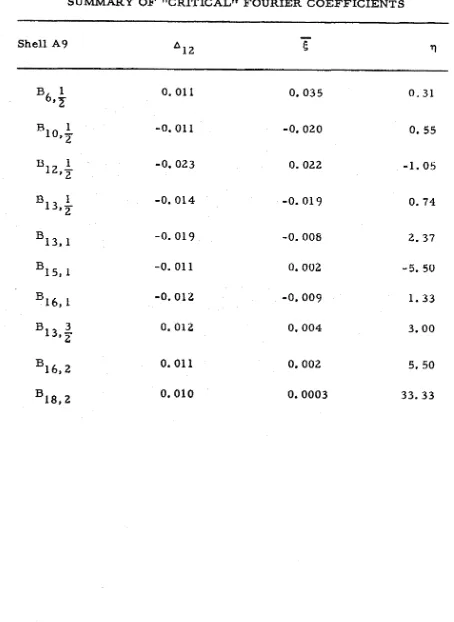
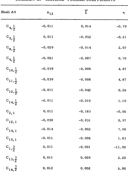
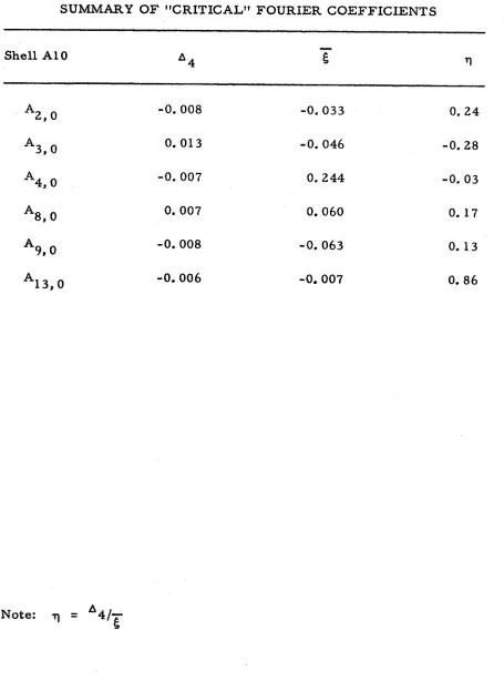
In an attempt to isolate the Iscritical modal c o r n p ~ n e n t s ' ~

-

defined a s those modal components which showed exponential growth

close to the c r i t i c a l load

-

harmonic analyses of the m e a s u r e d

imperfection s u r f a c e s were c a r r i e d out at each load level. In o r d e r

ta obtain the mathamat;ica;tl reprarssntatiwn that would d e s c r i b e "best" the m e a s u r e d imperfection s u r f a c e s different axial expansions w e r e

2 9

sine and the half wave cosine axial representations were calculated. This involved the computation of approximately 1,400 Fourier

coefficients for each complete scan. Detailed investigation of the rate of growth of these coefficients with increasing loading revealed that the consideration should be restricted to coefficients with a growth in excess of one per cent of the respective wall thicknesses a t the load level just before buckling. This would include all the coefficients which approach exponential growth at the experimental buckling load. Only about 40 of the computed Fourier coefficients showed significant growth rate and only about 20 of these showed exponential growth. All the coefficients that were investigated a r e summarized in Table V. Figures 40 through 44 show the rate of growth of three such "critical modal component^'^ for shells A7, A8, A9, A10, and A12 respectively. As can be seen from these figures most of these curves representing the experimentally measured

30

111.

COMPARISON

WITH THEORY

By tracing the growth of individual modal components of the measured imperfection surfaces during the loading process p r i o r to buckling it was discovered that for each shell tested several different modal components seemed to approach a horizontal tangent at about the experimental buckling load. It was, however, imp0 s sible to ascertain the exact value of loading a t the respective points of hori- zontal tangency just from observation of the given experimental data.

In considering the available theoretical methods it was found that none of them were quite general enough to be used directly with the measured experimental values. Koiter (Ref. 9 ) has presented an analytical procedure for obtaining the role of imperfections in imper- fection sensitive structures. Eater, working with an imperfection in the form of the radial displacement component of the axisymmetric buckling mode W = p cos(qox/R), he was able to show (Ref. 10) that

such an imperfection would reduce the buckling load of a cylindrical shell under axial compression to a s low a s one-third of the classical value for values of p. only a fraction of the shell thickness, How- e v e r , he conside red axisymmetric imperfections only.

In general, any radial imperfection pattern of the shell can be represented by a double Fourier s e r i e s in the axial and circumferen- tial coordinates. Thus in an effort to gain insight into the effects of the nonlinear interactions of several buckling modes an approximate

t e r m s of the double F o u r i e r s e r i e s , one axisyrnmetric and two a s y m m e t r i c ones. The approximate solution of the full nonlinear equations was obtained a s follows:

1 . The compatibility equation was solved exactly f o r the s t r e s s function F in t e r m s of the assumed r a d i a l displacement W and the m e a s u r e d imperfection

7.

This guaranteed that a kinematically admissible

displacement field would be associated with the solution of the second equation, the condition of equilibrium. 2 . The equation of equilibrium was solved approxi- mately by substituting t h e r e i n

I?,

W, and and then applying the Galerkin procedure,

It should be mentioned h e r e that a s i m i l a r method of solution has been u s e d by Hutchinson (Ref. 12). However he r e s t r i c t e d h i s i m p e r - fections to the f o r m of a l i n e a r buckling mode of the cylindrical shell. In the following solution this r e s t r i c t i o n was removed.

1. Donnell' s Shell Equations

Assuming that the radial displacement W is positive outward and that the m e m b r a n e s t r e s s resultants can be obtained f r o m an Airy s t r e s s function F a s

Nx

= F. W , N = F,xx and N = -F,

\ Y XY XY'

1 4 1 _{L (W, W}

₊

_{2 5 = 0}

E~

V

F -

x W , - +

2

where the nonlinear o p e r a t o r E is defined by

4

and P is the two-dimensional biharmonic o p e r a t o r , See Fig. 45 for notation.

2. Nonlinear Buckling Equations

The solution a s s u m e s initial imperfection shapes represented

-

_w

_=S;t

_{cos E +.f2t cos ~ ~ c o s &sin +}

_E

_m

_{~cos ~}

_&

_~

(2.1)

The equilibrium s t a t e of the axially loaded cylinder will be e x p r e s s e d a s :

W = 2 r t + w E

where the t e r m s added to w and f constitute the membrane p r e - buckling solution for the perfect shell. F u r t h e r , w will be assumed

a8

In the following approximate solution the effect of boundary conditions will b e neglected. Although in some instances the shell buckling m a y be characterized by certain end conditions, a s h a s been

shown by Hoff (Ref. 5) and Kobayashi (Ref. 6 ) , in t h i s solution only the effect of initial imperfections on the buckling load is of interest.

Substituting the a s s u m e d f o r m of W and into the compatibility equation (1. 1 ) yields

+

K4 s i n 2 E

+

K~ cos k z * cos

17 +

Kg

sin^

cos

17

+

K sin(i+k)Z cos

& +

K I O

9 sin(i-k)E cos

17

where the constants K1, K2,

. . .

.

,

K10 a r e defined in Appendix A. Since the boundary conditions of the finite shell will b e

neglected, therefore only a p a r t i c u l a r solution of equation ( 2 - 5 ) needs to be considered. To obtain such a p a r t i c u l a r solution l e t

t

F

sinkY 0 c o s

&

+

G cos(i+k)P cos

&

+

H

c o s ( i - k ) z cos

&

,

(2.7)

+

I sin(i+k)Z cos

$ +

J s i n ( i - k ) z * cos

&

The unknown coefficients A,

B y

. . . .

,

J a r e determined by substituting the assumed F into equation (2.5) and equating coefficients of like t e r m s . They a r e written out in detail i n Appendix A.

-

Substituting the assumed f o r m f o r

W,

W and the computed p a r t i c u l a r solution f o r F a s given by equations (2. I ) , (2.2) and (2.3) into the equilibrium equation (1. 2) yields the " e r r o r u

E N

=

tN

(f f f

X,ys).

Using Galerkin's idea of minimization of the " e r r o r f 1 1' 2' 3'

with r e s p e c t to a s e t of functions Beads to a s y s t e m of t h r e e nonlinear algebraic equations in the t h r e e unknowns f f f Here these

II

E ~ ( E ~ , E ~ , E ~ , I , ~ )

s i n

IS

cos

&

dF d T = 0 i

Imposing the r e s t r i c t i o n k =

_{2 '}

carrying out the indicated integra- tions and introducing the following nondimensional p a r a m e t e r s

2

a ₂ = (i-k) 2

_z(-E)

Rt 2 n 2

A solution of these "nonlinear equations" would yield the equilibrium

-

configuration of the finite shell a s a function of A . However for f

1

a r i d 5 s m a l l enough the e s s e n t i a l c h a r a c t e r of the shell in the p r e - buckling and the immediate po stbuckling configuration i s retained if the t e r m s of the o r d e r

g2,

5'1

and

c3

a r e omitted f r o m the previous

equations. Thus the following s y s t e m of simplified equations i s obtained:

3 . Buckling of a Perfect Shell:

z1

=

e2

=

c3

= 0 In this case the governing equations become

If C I > Cq9 there i s no deformation of a perfect shell in the

_--

buckling modes ($I =

e

-

e

= 0)until X reaches C4. Then the

2 - 3

coefficients of

5

and

c3

in equations. ( 3 . 2 ) and ( 3 . 3 ) vanish and a 2

bifurcation of the solution in the

c2

o r

g3

mode will occur. Since

-

g1

= 0, can be either positive o r negative. Suppose

e3

= 0, then following bifurcation h will decrease with deformation occurring in the

e2

a s well a s the negative axisymmetric mode

5

However if

eZ

= 0, 1 '

then following bifurcation h will decrease with deformation occurring in the

c3

and in the positive axisyrnmetric mode

cl.

In either case the maximum value of X attained i s at = C _4'

If C I

<

C q 9 there i s no deformation of a perfect shell in the

- -

buckling modes

(el

=

c2

=

e3

= 0) until h reaches CI. With h remain- ing at C1, deformation can occur in the axisymmetric mode; and

-

The bifurcated solution corresponds to decreasing values of X with deformation in both the

El

and

k2

modes. Similarly i f the axisym- m e t r i c deformation i s such that

5

₁ attains the value (C4

-

C 1 ) / 8

( C ₂

+

2C ₃ ) then the coefficient of

E3

in equation (3.3) vanishes and X decreases with deformation in both the

El

and

E3

modes. In either case the maximum value of X attained i s at A = C1. The behavior of the perfect shell i s shown in Fig. 4 6 .

4, Buckling of a Shell with h i s y m m e t r i c : Imperfection:

In this case the governing equations become:

Now if the imperfection i s purely axisymmetric then the prebuckling deformation i s also purely axisymmetric. Hence

E2

=

E3

= 0 which satisfies equations (4.2) and (4.3) identically and from equation ( 4 . 1)

-

F o r

E l

negative the prebuckling axisymmetric deformation

-

1

will be negative and bifurcation into the a s y m m e t r i c mode will occur when the coefficient of

e2

in equation (4.2) vanishes. That i s when

which is the equation of a straight line in the

A S l

-

plane. Following bifurcation the value of A d e c r e a s e s with deformation occurring in both the axisymmetric mode

cl

and the a s y m m e t r i c mode

E2.

F o r

5;

positive the prebuckling axisymmetric deformation

5

-

1

will be positive and bifurcation into the a s y m m e t r i c mode will occur when the coefficient of

gg

in equation (4.3) vanishes. That i s when

which i s the equation of another straight line in the

A t l

-

plane. Following bifurcation the value of X d e c r e a s e s with deformation occurring in both the axisymmetric mode

5

and the a s y m m e t r i c

]I

mode

g3.

This behavior of the shell i s shown in Fig. 47.

whe r e

5. Buckling of a Shell with Both Axisyrnrnetric and

-

Asymmetric Imperfections:

g1

f

0 and

%

f

0,

If

#

0,

5

#

0 and

5;

= 0 then the governing equations become:

In this c a s e deformation o c c u r s in both the

El

and

g2

modes for any nonzero values of X. Nonzero values of

c3

can occur only if the coefficient of

6

in equation ( 5 , 3 ) vanishes. Assuming that such

3

The t r a c e of the general solution curve in the AS2

-

plane can be obtained by 'eliminating between equations ( 5 . 4 ) and ( 5 . 5 ) . This yields

where

But this i s just a standard quadratic equation whose solution can be written down immediately a s :

-

Here the negative sign must be used for

e2

positive and the positive

-

A maximum value of A ( i f it o c c u r s ) i s associated with d X/de2 = 0. This condition along with equation ( 5 . 6 ) can be used to solve for AM. The result i s analogous to equation (4.7) but consider- ably m o r e complicated. Hence it i s m o r e convenient to obtain A M f r o m the X vs.

e2

plot using equation (5.8). This behavior of the

shell i s shown in Fig. 48.

-

If

-5

= 0 and d 3 L 0 then the governing equations

-

become:

Here deformation occurs in both the and

S3

modes for any 1

44

The t r a c e of the g e n e r a l solution curve in the hf

-

plane can be 3

obtained by eliminating

el

between equations (5. 12) and (5. 13). This yields

where

--

B2 =

(C,

*

C4

*

8c2f;)f3

+

C~ZJ

*8('z

*

C315153

The solution of t h i s standard quadratic equation can be written down immediately as:

-

The negative sign m u s t be used for

t3

positive and the positive sign

-

f o r f3 negative.

A maximum value of X(if it o c c u r s ) i s associated with

solve for

AM, However, a s pointed out e a r l i e r , it was found m o r e convenient to obtain XM f r o m the X vs.

E3

plot using equation (5. 16). This behavior of the shell i s shown in Fig. 48.

As expected, t h e introduction of the additional a s y m m e t r i c imperfection d e c r e a s e s the load carrying capacity of the shell even f u r t h e r . Thus the X M obtained f r o m the X vs.

E2

plot using

.

equation (5.8) o r f r o m the h vs.

Eg

plot using equation (5. 16) for a shell with both axisymmetric and a s y m m e t r i c imperfections will always be l e s s than the hM computed f r o m equation ( 4 . 7 ) for a shell with axisymmetric imperfection only.

6. Numerical Results

Equations ( 5 . 8 ) and (5.16) were programmed on the IBM 7094 and used in the s e a r c h for the "pair s f c r i t i c a l modal components", defined a s that combination of one axisymmetric and one asymrnetric imperfection component which gave the lowest value for

A M . In deriving the buckling equations (2. 11)

-

(2. 13) i t was n e c e s s a r y to impose the condition k = i/2 otherwise a11 the quad. r a t i c t e r m s in

El,

e2, and

E3

would vanish identically and the resulting buckling equations would describe a s y s t e m with stable postbuckled s t a t e s which a r e known to be insensitive to initial imperfections. Thus choosing an axisymmetric imperfection with wave number i automatically fixed the axial wave number k of the a s y m m e t r i c imperfection. Then

in

o r d e r to minimize the asyrn- m e t r i c buckling load h

=

C4 the circumferential wave number

1

I

2

a 2 + p - a = o

o r solving f o r

,I?:

with the r e s t r i c t i o n that for a positive, nonzero

whe r e

icJ = wave number s f the c l a s s i c a l axisyrnmetric buckling mode

The computation of the wave numbers is summarized i n Table VI for the shells tested. In actual u s e

$

was rounded to the n e a r e s t integer.

When combining t h e harmonic components of the experirnen- tally m e a s u r e d imperfection s u r f a c e s into p a i r s to be used a s input to the computer p r o g r a m s two s e p a r a t e c a s e s had to be considered.

-

Case a:

#

0 ,

5

/

0,

&

= 0

This resulted in coupling between the and

e2

modes and the input to equation (5.8) consisted of

*o i cos

E

"P

I

CkL sin kZ cos.& Coi s i n

K

-r

1

O1.1

-

s i n

k Z

sin

17

Case b:

f;

#

0,5

= 0,

T3

#

0

T h i s resulted in coupling between the and

t3

modes and the input to equation (5.16) consisted s f

Cke sin

k Z

cosf?? Aoi e cos

iF

--c

~d

sin kj; a sin

17

E O S k?? IJ C O S &

C

e s i n = - - +

o i

a cos kT 6 s i n e ?

It should be mentioned h e r e that the location s f the origin i n the circumferential direction was a r b i t r a r y , Thus either sine o r cosine

-

_{y-dependence was admissible.}

It was found that f o r a positive axisylmmetric imperfection coupling in the

5

mode would yield a lower value f o r A M then

3

_-

_-

coupling i n the

g2

mode if both

E2

and

E3

were of the s a m e size. Similarly f o r a negative axisymmetric imperfection coupling in the

48

49

IV.

CONCLUSION

Due to the s m a l l number of shells tested the r e s u l t s obtained thus f a r m u s t be considered only preliminary. However the follow- ing conclusions seemed to be warranted:

1. The initial imperfections of the shells surveyed so f a r w e r e c h a r a c t e r i z e d by being composed predominantly of lower o r d e r modes (i. e. few circumferential and even fewer axial waves). The

amplitudes of the higher o r d e r modes w e r e in general v e r y s m a l l (i. e. of the o r d e r of one p e r cent of the wall thickness o r l e s s ) .

2 . As can be seen f r o m the three-dimensional plots r e p r e s - enting the growth of the prebuckling deformations just p r i o r to

buckling (Figs. 28 through 3 1 ) t h e r e was a v e r y pronounced growth of imperfection components with long axial wave length and short

circumferential wave length f o r a l l the shells tested. The number of circumferential waves of these dominant components was approxima

-

tely equal to the number of circumferential waves in the postbuckled shape, The half wave length of the dominant components was equal to the length of the shell in the axial direction. However the axial half wave length of the postbuckled shape was much s h o r t e r than the axial half wave length of the dominant components in the prebuckling deformation.