Function-on-Function Regression with Public Health Applications
(Article begins on next page)
The Harvard community has made this article openly available.
Please share
how this access benefits you. Your story matters.
Citation
No citation.
Accessed
February 19, 2015 4:40:36 PM EST
Citable Link
http://nrs.harvard.edu/urn-3:HUL.InstRepos:12274591
Terms of Use
This article was downloaded from Harvard University's DASH
repository, and is made available under the terms and conditions
applicable to Other Posted Material, as set forth at
http://nrs.harvard.edu/urn-3:HUL.InstRepos:dash.current.terms-of-use#LAA
Function-on-Function Regression with Public
Health Applications
A dissertation presented
by
Mark John Meyer
to
The Department of Biostatistics
in partial fulfillment of the requirements
for the degree of
Doctor of Philosophy
in the subject of
Biostatistics
Harvard University
Cambridge, Massachusetts
May 2014
c
2014 - Mark John Meyer
Dissertation Advisor: Professor Brent A. Coull Mark John Meyer
Function-on-Function Regression with Public
Health Applications
Abstract
Medical research currently involves the collection of large and complex data. One such type of data is functional data where the unit of measurement is a curve measured over a grid. Functional data comes in a variety of forms depending on the nature of the research. Novel methodologies are required to accommodate this growing volume of functional data alongside new testing procedures to provide valid inferences. In this dissertation, I propose three novel methods to accommodate a variety of questions involving functional data of multiple forms. I consider three novel methods: (1) a function-on-function regres-sion for Gaussian data; (2) a historical functional linear models for repeated measures; and (3) a generalized functional outcome regression for ordinal data. For each method, I discuss the existing shortcomings of the literature and demonstrate how my method fills those gaps. The abilities of each method are demonstrated via simulation and data application.
Contents
Title page . . . i Abstract . . . iii Table of Contents . . . iv List of Figures . . . vi List of Tables . . . x Acknowledgments . . . xii1 Bayesian Function-on-Function Regression for Multi-Level Functional Data 1 1.1 Introduction . . . 2
1.2 Function-on-Function Regression Model for Multi-Level Functional Data . . 5
1.2.1 General Basis Transform Modeling Approach . . . 6
1.2.2 Model Formulation . . . 8
1.2.3 More Complex Function-on-Function Mixed Models . . . 11
1.3 Posterior Functional Inference . . . 12
1.4 Simulation . . . 14
1.5 Application . . . 19
1.5.1 Description of ERP Data Set . . . 19
1.5.2 Analysis . . . 20
1.6 Discussion . . . 25
2 Bayesian Historical Functional Mixed Models for Repeated Measures 31 2.1 Introduction . . . 32
2.2 Historical Functional Mixed Models . . . 35
2.2.1 Model Formulation with Wavelets . . . 36
2.2.2 Historical Constraint via Wavelet-Packets . . . 38
2.3 Posterior Functional Inference . . . 44
2.4 Simulation . . . 46
2.5 Example: Boilermaker Study . . . 49
2.6 Discussion . . . 52
3 Ordinal Probit Wavelet-based Functional Models for eQTL Analysis 57 3.1 Introduction . . . 58
3.2 Ordinal Probit Functional Model . . . 60
3.2.1 Wavelet-based Modeling of the Latent Outcome . . . 62
3.2.2 MCMC Algorithm . . . 65
3.2.3 Posterior Functional Inference . . . 67
3.3 Extension to Generalized Function-on-Function Regression . . . 69
3.4 Simulation . . . 71
3.5 Application . . . 79
3.6 Discussion . . . 85
Appendices 90 A.1 Bayesian Function-on-Function Regression for Multi-Level Functional Data 91 A.1.1 MCMC Sampler . . . 91
A.1.2 Additional Simulation Details . . . 93
A.1.3 Additional Application Results . . . 95
A.2 Bayesian Historical Functional Mixed Models for Repeated Measures . . . . 97
A.2.1 MCMC Sampler . . . 97
A.2.2 Additional Simulation Details . . . 98
A.3 Ordinal Probit Wavelet-based Functional Models for eQTL Analysis . . . . 100
A.3.1 Additional Simulation Details . . . 100
A.3.2 Additional Results for SNPs within 250kb of IREB2 . . . 101
List of Figures
1.1 Heat maps of the true surfaces for simulation study are in the top row. The
bottom row contains estimated surfaces for each simulated scenario based
on a sample size ofn = 25with two measure per subject,Ci = 2∀i, for a
total ofN = 50 observations. Each surface is the average of the posterior
estimate for the true surface based on 200 simulated datasets. . . 16
1.2 On the left, raw profile curves are plotted in gray with the mean in red from
electrode 129 under the cigarette image condition. On the right, are raw
curves and the mean from electrode 129 under the neutral image condition. 20
1.3 The top row contains surface estimates for the association between
elec-trodes 129 and 55. Posterior surfaces comparing elecelec-trodes 11 to 75 are in the second row. The estimated posterior surface of the difference between cigarette and neutral is found in the first column. Group specific surface estimates are in the second and third columns, Neutral and Cigarette re-spectively. ERP output from electrode 129 is the response and the output from electrode 55 is the predictor for the first model and electrode 75 is the predictor of electrode 11 in the second model. . . 22
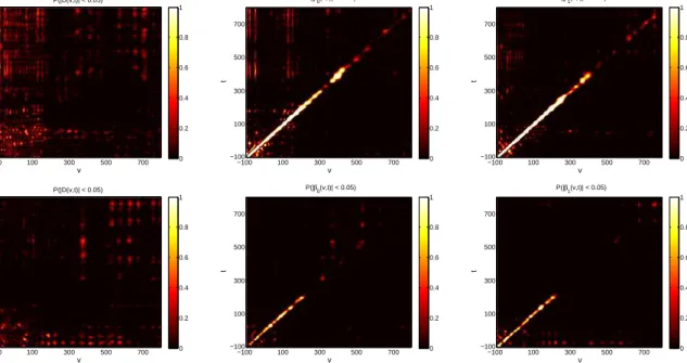
1.4 Heat maps containing the posterior probabilities from the BFDR procedure
usingaδintensity change of 0.05. Coefficients in white have a high
proba-bility of being greater thanδ and thus likely to be included inψ, the set of
coefficients flagged as significant. Black coefficients have a low probability
of being greater thanδand are thus less likely to be flagged as significant.
The top row contains results from the model using electrodes 129 and 55 while the second row contains results from the model using electrodes 75 and 11. . . 23
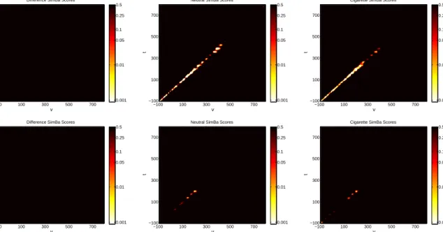
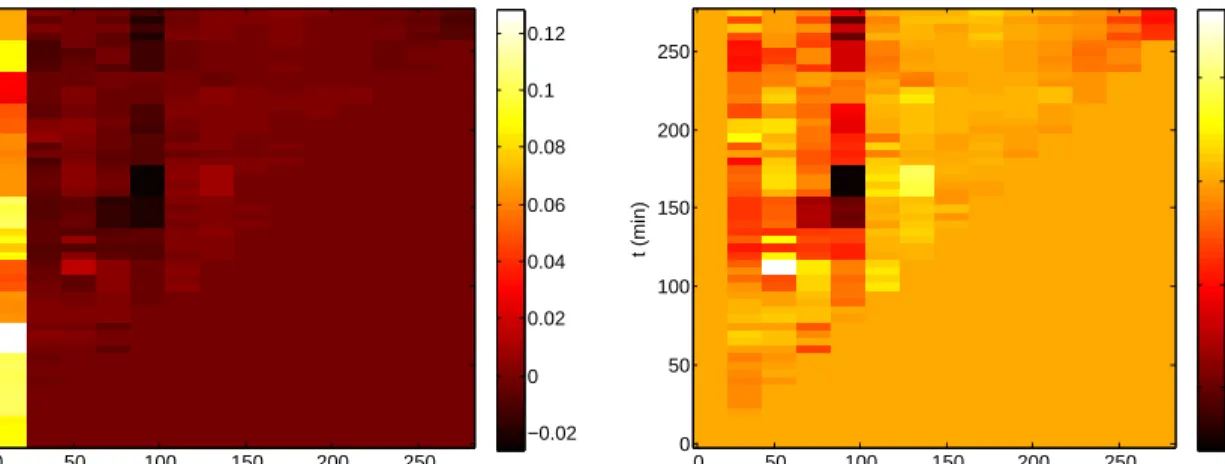
1.5 Heat maps containing the SimBa scores for each surface of both models.
The top row contains results from the model using electrodes 129 and 55 while the second row contains results from the model using electrodes 75
and 11. Scores are plotted on thelog-scale with the color axis on the
expo-nential scale. White regions represent coefficients with low SimBa scores, black regions represent coefficients with high SimBa scores. . . 24
2.1 Boilermaker Study HRV and PM exposure profiles. Individual subject
pro-files are in gray, the mean of across time is in red. Time is measured as minutes from the start of measurement. . . 34
2.2 (a) Decomposition of a function x(t)into three levels using DWT, x(t) =
A3 +D3 +D2+D1. (b) Graphical representation of the decomposition of
a function into three levels using DWPT,x(t) = AAA3 +AAD3 +ADA3 +
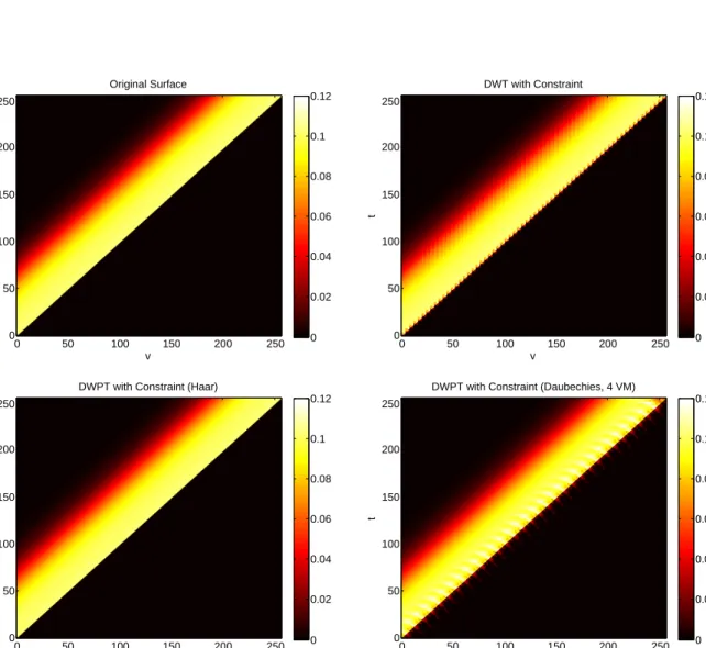
2.3 Proof of concept of the historical constraint. Top left: original image. Top right: decomposed and reconstructed original image with constraint in wavelet space. Bottom left: decomposed and reconstructed original im-age with constraint in wavelet-packet space using Haar wavelets. Bottom right: wavelet-packet space proof of concept using Daubechies wavelets with 4 vanishing moments. . . 41
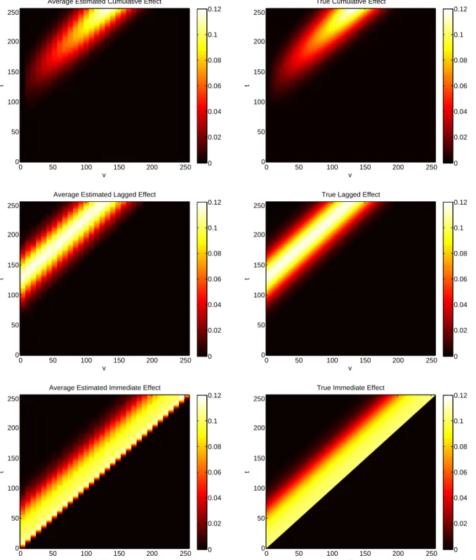
2.4 Left column: heat maps of average estimatedβ(v, t)plotted as functions of
tand v based on a sample size ofn = 45withN = 150total curves. Right
column: heat maps of the trueβ(v, t)functions plotted as functions oftandv. 47
2.5 Left: the full estimated surface from the Boilermaker Study using PM2.5 as
the exposure and SDNN as the outcome. Right: estimated surface remov-ing associations with minimal to no precedremov-ing exposure. Time scale is in minutes since the start of measurement. Both exposure and outcome were
log-transformed prior to modeling. . . 50
2.6 Posterior probabilities of the coefficients of the estimated surface for two
levels of δ. The left contains the heat map of a low δ intensity change of
0.005 while the right heat map contains a high δ intensity change of 0.02,
high and low relative the surface. . . 51
3.1 Posterior estimates ofβ(t)as a function of t averaged over 200 simulated
data sets for a single covariate. Light gray bands depict the 95th percentile across the simulated data sets, true functions are in solid dark gray. The top row contains estimates for the single peak scenarios, bottom row contains double peak. . . 74
3.2 The figure on the left contains the average point-wise bias of the estimated
β(t)as a function of t taken across 200 simulated data sets. The figure on
the right compares box plots across scenarios of rMSE calculated for each simulated data set. . . 75
3.3 Posterior estimates ofβ(t)as a function of t averaged over 200 simulated
data sets for a single covariate. Light gray bands depict the 95th percentile across the simulated data sets, true functions are in solid dark gray. The top row contains estimates for the single peak scenarios, bottom row contains double peak. . . 76
3.4 Left column: heat maps of FDRεas functions ofεfor the BFDR with varying
levels of πδ. Right column: heat maps of SENΥ as functions of Υ for the
BFDR with varying levels ofπδ . . . 78
3.5 Plotted SENΥas functions ofΥfor the SimBaS procedure. Each single
co-variate scenario is depicted as described in the legend. . . 79
3.6 Single probe models SimBa Scores plotted as functions of position on the
chromosome. The location of IREB2 is noted as a horizontal bar below the probabilities. For convenience, a dotted-dashed gray line depicts a global
3.7 Joint model SimBa Scores plotted as functions of position on the chromo-some. The location of IREB2 is noted as a horizontal bar below the
proba-bilities. For convenience, a dotted-dashed gray line depicts a globalα-level
of0.05plotted on the−log10scale. . . 82
A.1 Heat maps of proposed “true” surfaces for simulation study are in the top row, equations found in Models (3.2) - (3.5). The surfaces are estimated
based on a sample size ofn = 100with repeated measures giving a total of
N = 200observations. . . 94
A.2 Boxplots comparing the root-Mean Square Error amongst varying sample sizes by simulation scenario. Not surprisingly, as sample size increases, rMSE decreases. Note that the graphics are listed by total number of
obser-vations withN = 50on the left andN = 200on the right. . . 94
A.3 Each figure contains a heat map displaying the FDR acceptance region av-eraged over 200 simulated data sets. The dark red regions indicate coeffi-cients flagged in every or almost every data set. Dark blue coefficoeffi-cients were not flagged in any or almost any data sets. At the edge of each flagged re-gion, coefficients that were flagged only occasionally can be seen. These
figures were based on the smallest sample sizeN = 50,n= 25. . . 94
A.4 Each figure contains a heat map displaying the SimBa Scores. All plots are
on thelog-scale, however for interpretability, the color scale has been
expo-nentiated. For consistency of interpretation, the color scale was reversed so that the darker the red the more significant the coefficient and the darker the blue, the less significant. The scale is set to exhibit the variation in the SimBa Scores over the region of elevated significance. As such, the max of the scale does not accurately reflect the SimBa Scores where the true sur-face lacks association. Each plot represents the average SimBaS for each coefficient over the 200 simulated data sets. These figures were based on
the smallest sample sizeN = 50,n = 25. . . 95
A.5 Heat maps of the set of flagged locations (v, t), ψ, from the BFDR.
Sig-nificant locations appear in white, non-sigSig-nificant locations are in black.
For the difference surface, α = 0.05while the image-specific surfaces use
α = 0.025. Theδ-intensity change is 0.05 for all surfaces. The top row
con-tains results from the model using sensors 129 and 55. The bottom row contains results from the model using sensors 75 and 11. . . 95
A.6 Heat maps of the set of flagged locations (v, t) using PWCI. Locations in
white were flagged as significant by the procedure while locations in black are not-significant. The top row contains results from the model using sen-sors 129 and 55. The bottom row contains results from the model using sensors 75 and 11. . . 96
A.7 Boxplots of rMSE by total sample size. ForN = 150, there were onlyn= 45
A.8 Left column: heat maps of average estimatedβ(v, t)plotted as functions of
tandv based on a sample size ofN =n = 1000. Right column: heat maps
of the trueβ(v, t)functions plotted as functions oftandv. . . 99
A.9 Left column: heat maps of FDRεas functions ofεfor the BFDR with varying
levels of πδ. Right column: heat maps of SENΥ as functions of Υ for the
BFDR with varying levels ofπδ . . . 100
A.10 Joint 95% credible bands for each single probe set model. Bands are calcu-lated in the manner describe both in the paper and in Ruppert, Wand, and Carroll (2003). . . 101 A.11 Joint 95% credible bands for each probe set from the joint model. Bands are
calculated on each probe set separately in the manner describe both in the paper and in Ruppert, Wand, and Carroll (2003). . . 102 A.12 Single probe models SimBa Scores plotted as functions of position on the
chromosome. The location of IREB2 is noted as a horizontal bar below the probabilities. For convenience, a dotted-dashed gray line depicts a global
α-level of 0.05 plotted on the −log10 scale. Scores are from the models
taking 2Mb to either side of IREB2. . . 103 A.13 Joint model SimBa Scores for the probe sets 1555476 at, 214666 x at, and
242261 at plotted as functions of position on the chromosome. The loca-tion of IREB2 is noted as a horizontal bar below the probabilities. For
con-venience, a dotted-dashed gray line depicts a globalα-level of0.05plotted
on the −log10 scale. Scores are from the models taking 2Mb to either side
of IREB2. . . 104 A.14 Joint 95% credible bands for each probe set from the joint model for 1555476 at,
214666 x at, and 242261 at. Bands are calculated on each probe set sepa-rately in the manner describe both in the paper and in Ruppert, Wand, and Carroll (2003). . . 105
List of Tables
1.1 FDR, sensitivity, experiment-wise error rate (EWER), and type I error
val-ues by inference procedure. The BFDR use aδintensity change of0.05. To
determine assessment values for SimBaS, a cutoff of α = 0.05 was used.
Likewise, the PWCI used 95% point-wise credible intervals to determine
significant locations. . . 18
2.1 FDR, sensitivity and, experiment-wise error rate values by inference
pro-cedure. BFDR was calculated with aδof0.05and a globalαof0.05. . . 49
3.1 Significant SNPs from joint model by expression probe set. Significance
based on joint model SimBa Score exceeding the global alpha of0.05. Joint
model scores are also compared to single probe scores for the same SNP
as well as BFDR probabilities from the joint model for three different πδ
values. 1 denotes SNPs significantly associated with both 1555476 at and
Acknowledgments
I would like to first thank my parents, Kent and Deb, and my sister, Serenity, whose love and support over the years brought me through tough times. I’d like especially thank my advisor, Brent A. Coull, who has served as a wonderful mentor over the last five years and without whom none of this would be possible. Next, I’d like to thank my previous mentors, Monica Jackson, Gang Zheng, and Elizabeth (Betty) J. Malloy, without whom I would not be where I am. In particular, I’d like to give additional thanks to Betty who inspired me to pursue statistical research, encouraged me to apply to graduate school, served on my committee, and continues to be a mentor, collaborator, and friend. To the remaining members of my committee, Christoph Lange and Craig P. Hersh, thank you for your contributions to this dissertation and the knowledge you’ve imparted. I’d like to give special thanks to Matt Cefalu, Natalie Exner, Lauren Kunz, Shira Mitchell, and Elizabeth Smoot who all have provided an abundance of moral support over the past few years. Finally, I’d like to thank my friends and extended family who have supported me over these years.
1. Bayesian Function-on-Function Regression for
Multi-Level Functional Data
Mark J. Meyer
1, Brent A. Coull
1, Francesco Versace
2, Paul Cinciripini
2,
and Jeffrey S. Morris
21
Department of Biostatistics, Harvard School of Public Health
1.1
Introduction
Medical and public health research increasingly involves the collection of complex and high dimensional data. In particular, functional data—where the unit of observation is a curve or set of curves that are finely sampled over a grid—is frequently obtained (Ram-say and Silverman, 2005). Moreover, researchers often sample multiple curves per subject which yields repeated functional measures. A common question is how to analyze the re-lationship between two functional variables. While the field of functional data analysis (FDA) has progressed considerably in recent years, gaps remain in the literature with re-gards to function-on-function regression where both the predictor and outcome are func-tional.
Regression in FDA can be classified into three broad sub-classes: scalar-on-function, function-on-scalar, and function-on-function. Classical functional regression, on which a large literature exists, involves scalar-on-function regression where the outcome is scalar and the predictor is functional, with functional regression coefficients. See for in-stance Ramsay and Dalzell (1991), Cardot, Ferraty, and Sarda (1999), Reiss and Ogden (2007), Malloy et al. (2010), Goldsmith et al. (2011), McLean et al. (2012), Gertheiss, Maity, and Staicu (2013), and references therein. Function-on-scalar regression, also heavily in-vestigated in the literature, involves regressing a functional predictor on to a set of scalar covariates, each of which has a functional regression coefficient. See for instance Brum-back and Rice (1998), Morris and Carroll (2006), Reiss, Huang, and Mennes (2010), Staicu et al. (2011), Chen and M ¨uller (2012), Goldsmith, Greven, and Crainiceanu (2013), and references therein.
In contrast, the literature addressing function-on-function regression, with functional outcome, functional predictor, and a coefficient surface, is rather sparse. Much of it is dedicated to the historical functional linear model (HFLM), as described by Malfait and Ramsay (2003) and further examined by Harezlak et al. (2007) and Kim, S¸ent ¨urk, and Li (2011). The primary assumption in an HFLM is that the association between curves is
uni-directional, which leads to a upper triangular regression surface. That is, for func-tions of time, an association between the predictor at any given time-point can only occur with the outcome at subsequent times. Function-on-function regression allowing for bi-directional associations—that is, with unconstrained regression coefficient surfaces—is explored by Yao, M ¨uller, and Wang (2005) and M ¨uller and Yao (2008).
There are some recent technical reports on the topic from one research group, Ivanescu et al. (2012), Scheipl and Greven (2012), Scheipl, Staicu, and Greven (2014), that discuss a penalized spline approach, identifiability issues, and function-on-function regression in Functional Additive Mixed Models, respectively. One major limitation to both Scheipl and Greven (2012) and Scheipl, Staicu, and Greven (2014) is the assumption of iid errors which might be unrealistic for functional data. Ivanescu et al. (2012) do allow for corre-lated errors, but only present results assuming iid errors. Additionally, neither Scheipl and Greven (2012) nor Ivanescu et al. (2012) account for correlation induced by multiple measurements on the same subjects and while Scheipl, Staicu, and Greven (2014) do incor-porate a random functional effects, they cannot incorincor-porate correlation between different
random effects. Ivanescu et al. (2012) and Scheipl, Staicu, and Greven (2014) address
inferential procedures, relying on 95% point-wise confidence intervals (PWCI) to deter-mine significance. Neither approach, however, makes any adjustment for the multitude comparisons.
To motivate our development of the function-on-function setting, we examine data from a smoking cessation trial, conducted in the Department of Behavior Sciences at the Univer-sity of Texas M. D. Anderson Cancer Center (Cinciripini et al., 2013). For a subset of par-ticipants, researchers obtained Event Related Potentials (ERPs) at baseline during the pre-sentation of a series of images depicting neutral, positive, negative, and cigarette-related contents. ERPs were collected using a 129 channel Geodesic Sensor Net. Finely sampled curves were produced over the course of 900 ms (100 ms prior to picture presentation and 800 ms after). Electrical potentials every 4ms were collected from 129 electrodes dis-tributed on the surface of the scalp resulting in 225 measurements for each electrode.
While many analyses are of interest for these data, in this paper we focus on characteriz-ing the time-varycharacteriz-ing relationship between ERP outputs from pairs of electrodes.
In this paper, we propose a general function-on-function regression modeling frame-work that can accommodate this type of multilevel functional data. The model is flex-ible enough to incorporate a variety of basis expansions including such common ap-proaches as principal components, spline-based and wavelet-based functional represen-tations. Our approach not only allows for correlation between functions through random effect functions, but also allows heteroscedasticity and within-function correlation in the residual error functions. While the approach can be applied generally for any number of functional predictors and arbitrary interactions with other discrete and continuous pre-dictors, we present specific model formulations for both a single functional predictor of interest as well an interaction of a discrete factor with a functional predictor which re-sults in separate function-on-function regressions for each discrete factor. For inference, we propose three approaches. First we extend the Bayesian False Discovery Rate (BFDR) procedure proposed by Morris et al. (2008) to the function-on-function setting. Second, we generate joint credible bands as in Ruppert, Wand, and Carroll (2003). Next we gener-ate two novel Bayesian summaries: (1) Simultaneous Band Scores (SimBaS), a functional measure we introduce that summarizes for each position in the regression surface the
smallest αfor which the 100(1−α)% joint credible bands exclude zero at that position,
and (2) Global Bayesian P-Values (GBPV), which can be interpreted as a type of Bayesian p-value corresponding to a global functional null hypothesis of no relationship between the functions. These summaries are of general interest and can be used in other functional regression settings.
Section 1.2 develops a simple version of our proposed function-on-function mixed model, presents a more general model, and describes our basis function modeling strategy. Sec-tion 1.3 details the BFDR, SimBaS, and GBPV inference procedures. In SecSec-tion 1.4 we present the results of a simulation assessing model fit and the BFDR, SimBaS, and GBPV procedures. Section 1.5 presents the results obtained by applying the proposed methods
to the ERP data, and Section 1.6 contains further discussion.
1.2
Function-on-Function Regression Model for
Multi-Level Functional Data
Here we introduce the function-on-function model we will use to regress one function
y(t), t∈ T on anotherx(v), v ∈ V. First we consider a simple case with a single functional
predictor and repeated measures of{y(t), x(v)}pairs for each subject, and then in Section
1.2.3 we describe more complex models that can be handled by our approach.
Individual subjects are denoted as i = 1, . . . , n. Letc = 1, . . . , Ci index repeated pairs of
curves observed on subjecti. Then for subjecti, curve setc, we observexic(v)andyic(t),
{yic(t), xic(v) :t∈ T, v ∈ V},
yic(t) =α(t) +
Z
v∈V
xic(v)β(v, t)dv+Ui(t) +Eic(t). (1.1)
We assume observation-specific and subject-specific Gaussian process errors Eic(t) ∼
GP(0,ΣE) and Ui(t) ∼ GP(0,ΣU). The integration over the entire support of v allows
the exposure-response relationship to move in either direction, i.e. we do not assume
the timing of an effect ofxonyoccurs in one direction or the other. That relationship is
characterized by the surfaceβ(v, t).
In this paper, our focus is on functional data sampled on a common fine grid. Here,
we consider a discretized version of Model (1.1). Let yic(·)be finely sampled on a grid
t= [t1 · · · tT]of lengthT. Similarly,xic(·)is observed on a gridv= [v1 · · · vV]of lengthV.
We can then define the row vectorsyic = [yic(t1) · · · yic(tT)] andxic= [xic(v1) · · · xic(vV)]
and express Model 1.1 in the discrete form
yic =xicβ+ui+eic (1.2)
whereyic,ui, andeicare1×T,xicis1×V, andβis theV ×T matrix of coefficients. Note
then thateic ∼ N(0,ΣE)and ui ∼ N(0,ΣU). In practice, we center and scale both yic(t)
Now letN be the total number of observed response curves. Stacking the row vectors by
subject,YandXrepresent theN ×T andN ×V matrices of observed curves. Further,Z
is theN ×nrandom effects design matrix. Our discretized model for all subjects is then
Y=Xβ+ZU+E (1.3)
whereβis as defined in Model (1.2),U is then×T matrix of subject specific random effect
functions on the grid, andEis theN ×T matrix of model errors, interpretable as residual
curve-to-curve deviations.
Because of the functional nature of the data, we do not directly fit Model (1.3). Instead, we represent the curves using some basis function expansion and apply basis
transfor-mations to y(t) and x(v)prior to model fitting. This basis function transform approach
has numerous advantages, including dimension reduction, more efficient computation, and borrowing of strength across observations of the curves. Previous work in the func-tional regression context has used a variety of basis functions including kernels, splines, wavelets, and functional Principal Components (fPC). We will begin by presenting a gen-eralized basis expansion for our model to demonstrate how multiple candidate transfor-mations can be used in our model. Then we will present the rest of the modeling details using specific basis functions chosen for our simulation and data analysis, with the un-derstanding that it can be adapted for use with other basis functions.
1.2.1
General Basis Transform Modeling Approach
Here we describe our general basis function transform approach for fitting the function-on-function regression models, which involves projecting both the functional responses and predictors into a chosen basis space, fitting the model in the basis space, and then transforming the results back to the original function space for interpretation and infer-ence. Let yic(t) = PT ∗ j=1y ∗ icjξj(t) and xic(v) = PV ∗ j=1x ∗
expansion for the functional responses and predictors, respectively. Potential choices in-clude wavelets, B-splines, kernels, Fourier bases, principal components, or independent
components. Letξbe a matrix of sizeT∗×T containing the basis functions on the discrete
gridtwith element(i, j)given byξi(tj), and likewise letφbe aV∗×V matrix containing
the basis functions forx(v)evaluated on the gridv. Considering the discretely sampled
functions in matrix form, we can write the basis expansion asY=Y∗ξandX=X∗φ, with
Y∗andX∗beingN×T∗andN×V∗matrices, respectively, containing the basis coefficients
for the observed functions. Here we assume thatφandξare of full row rank, possibly but
not necessarily orthogonal, so rank(φ) =V∗, rank(ξ) =T∗ and φφ0 andξξ0 are invertible
matrices of sizeV∗×V∗ andT∗×T∗, respectively.
Replacing each functional quantity in Model (1.3) with its basis expansion, we have
Y∗ξ =X∗φφ0β∗ξ+ZU∗ξ+E∗ξ, (1.4)
whereβ∗isV∗×T∗,U∗ isn×T∗, andE∗isN×T∗, representing quantities of Model (1.3)
in the transformed basis space. Whenφ is orthogonal so thatφφ0 = IV∗, if we multiply
each side of (1.4) byξ− =ξ0(ξξ0)−1, then we arrive at thebasis space model
Y∗ =X∗β∗+ZU∗+E∗. (1.5)
When φis not orthogonal, we instead replace β∗ in Model (1.5) withβ† = φφ0β∗. Thus,
we can fit this basis space model after first transforming the functional responses and
pre-dictors to their respective basis spaces,Y∗ =Yξ− andX∗ =Xφ−, withφ− =φ0(φφ0)−1, and
then after fitting the model, transform back to the original function space to obtain
esti-mates and inference forβ =φ0β∗ξwhenφis orthogonal,β =φ−β†ξotherwise. Note that
for some choices of basis functions, fast transform algorithms can be used in lieu of ma-trix multiplication to compute the basis functions or transform back to the original space, e.g., discrete wavelet transform (DWT) for wavelets, discrete Fourier transform (DFT) for Fourier bases, and fast algorithms for computing independent components (Hyvarinen et al., 2001).
We take a Bayesian approach to fit Model (1.5), using an Markov Chain Monte Carlo (MCMC) procedure to sample from the posterior distributions using appropriate prior distributions for each model parameter. The specifics of the sampler may vary slightly depending on choice of basis function, and will be described in Web Appendix A. This formulation allows a variety of possible basis functions to be used for the outcome and predictor, including variations of wavelets, principal components, Fourier series, and
splines, each of which corresponds to different choices of ξ and φ. For example, for
wavelets ξ and φ are inverse discrete wavelet transform (IDWT) matrices, for principal
components they are the eigenvectors, possibly rescaled by the eigenvalues, for Fourier series they are the Inverse Discrete Fourier Transform (IDFT) matrices, and for splines they can be constructed based on B-splines or orthogonalized B-spline design matrices.
Note that the same basis transform does not need to be used for bothy(t)andx(v). In this
paper, we use wavelet bases to represent the functional form ofy(t), and forx(v), we use
a composite strategy involving wavelets followed by principal components that we refer to as wPC, which is similar to strategies used by Johnstone and Lu (2009) and Røislien and Winje (2012).
1.2.2
Model Formulation
Here, we present our modeling details using wavelets fory(t)and wPC forx(v). First, we
transform the functions to the wavelet space by applying theO(T)DWT to each row ofY
andX, which can be represented as
yic DWT−→yWic ={yic,jkW }andxic DWT−→xWic ={xWic,s`}.
Wavelets are multi-resolution bases that are double-indexed by scale and location. The
scales arej = 1, . . . , Jy ands= 1, . . . , Sxand locationsk = 1, . . . , Ky
j and`= 1, . . . , Lxs for
Y andX, respectively. The dimension of yW
ic is1×T W where TW = PJy j=1k y j. Similarly, xW
ic has dimensions 1×VW where VW =
PSx
s=1`
x
s. If T and V are powers of two, this
padding is done according to some chosen boundary condition (e.g. periodic, reflection,
and padding with zeros), in which caseTW andVW are not exactly equal to but are of the
same order asT andV. We discuss choice of padding further in our simulation study in
Section 1.4.
Wavelets tend to provide sparse representations for many functions, so one can achieve data compression by eliminating wavelet coefficients that are negligible in magnitude for all curves. Wavelet thresholding has been widely used for compression and denoising
of individual functions, and Morris et al. (2011) introduced ajoint compressionapproach
for the multiple function setting that finds a minimal subset of wavelet coefficients that
jointly preserves 100α% of the total energy for all functions in a set. Let TW∗ and VW∗
represent the total number of coefficients left after such joint compression.
We can write these wavelet basis expansions in matrix form asY=YWWyandX=XWWx,
whereWyandWxareTW
∗
×T andVW∗×V matrices, respectively, containing the retained
wavelet basis functions evaluated on theT andV grids. Given orthogonal wavelets, we
can also represent the DWT in matrix form as YW = YWy0 and XW = XWx0, or if
non-orthogonal they can be representedYW =YWy−andXW =XWx−. Thus, in the notation of
Section 1.2.1, if we use wavelet transforms with joint compression for bothy(t)andx(v),
then we effectively defineξ =Wy andφ =Wx, withξ− =Wy0 andφ−=Wx0,Y
∗
=YW and
X∗ =XW, andT∗ =TW∗ andV∗ =VW∗.
In our model, calculations are linear inT∗ but quadratic inV∗, so dimension reduction in
X∗has especially important computational benefits. While the joint compression provides
some dimension reduction, use of Principal Components Analysis (PCA) can provide additional dimension reduction. In particular, consider performing the singular value
decomposition of XW = XWx0 = QΣP0. Noting that XW isN ×VW∗, we see that Q, the
matrix of left singular vectors, is N ×VW∗ and both Σ, the diagonal matrix of singular
values, andP, the matrix of right singular vectors, areVW∗×VW∗. Supposing we keep
Vsvd VW∗ principal components, we can compute the wavelet-space PC scores X∗
XWPsvd, wherePsvd is a VW
∗
×Vsvd matrix computed from the leadingVsvd rows of P.
Using the notation of Section 1.2.1, this composite basis function strategy is equivalent
to computing X∗ = Xφ− with composite transform φ− = Wx0Psvd and inverse transform
φ = Psvd0 Wx of dimension V∗ = Vsvd. Note that one could simply define φ to be the
eigenvectors of a direct SVD on X, but this composite wPC approach has advantages
in that the joint compression in the wavelet space (1) reduces the dimensionality of X
to speed up calculation of the SVD, (2) performs some denoising of the functions in X
before calculation of the SVD, and (3) borrows strength locally within the function, thus accounting for the functional nature of the data.
Thus, after transforming the data, recall our basis space model (1.5) is given by Y∗ =
X∗β∗+ZU∗+E∗. Consistent with previous work (Morris and Carroll (2006), Morris et al.
(2008), Zhu, Brown, and Morris (2011), among others), we assume independence in the
wavelet space. That is, for the subject specific version of Model (1.5),y∗ic =x∗icβ∗+u∗i+e∗ic,
we assumee∗ic ∼ N(0,Σe∗) where Σ∗e is a diagonal matrix with elements varying by j, k,
Σ∗e = nσe2(j,k)o, and equivalently u∗
i ∼ N(0,Σ∗u)where Σ∗U =diag
n
σU2(j,k)o. The induced
within-function covariances in the data space are given byΣe = ξ0Σ∗eξ and Σu = ξ0Σ∗uξ,
which with wavelets accommodates a broad class of covariances allowing heteroscedas-ticity and differing degrees of autocorrelation, and thus different degrees of borrowing of strength, in different regions of the function (Morris and Carroll, 2006; Morris, et al. 2008; Morris, et al. 2011). When other basis functions are used, one must consider whether the class of induced covariance structures from basis space independence is sufficiently flex-ible to capture the key functional features, with other parsimonious alternatives possflex-ible, for example serial correlation across neighboring basis coefficients.
The basis space independence assumption allows us to split Model (1.5) into a series ofT∗
separate models for each basis coefficient in they-space, double-indexed by(j, k), giving
y∗(j,k) =X∗β(∗j,k)+Zu∗(j,k)+e∗(j,k), wherey∗(j,k) ande∗(j,k)areN ×1,β(∗j,k)isV∗×1, andu∗(j,k)
is n ×1. X∗ and Z are as previously defined. This separability allows computational
frequently yield T∗ T, and when cluster computing resources are available, allows
parallel computing across(j, k). For prior specification, we assume vague proper priors
on the variance components and a spike-and-slab prior similar to that found in Morris and Carroll (2006), Malloy et al. (2010), and others (see Web Appendix A for details).
Posterior samples are then generated forβ∗and projected back into the data-space using
β =φ−β∗ξ, where recall for our example φ− = φ0 =Psvd0 Wxand ξ =Wy. These posterior
samples are used to perform Bayesian inference onβ, as detailed in Section 1.3.
1.2.3
More Complex Function-on-Function Mixed Models
The simple function-on-function regression Model (1.1) is a special case of a general
function-on-function mixed model that incorporates arbitrary scalar covariates{Xa, a =
1, . . . , ps}, functional covariates {Xa(va), a = 1, . . . , pf}, scalar-by-function interactions,
and multiple levels of random effect covariates{Zh
l, h = 1, . . . , H;l = 1, . . . , Lh}. In
prin-ciple, our approach can also accommodate function-by-function interactions, but we omit that here. The general model can be written
yi(t) = ps X a=1 XiaBa(t) + pf X a=1 Z va∈Va Xia(va)βa(va, t)dva + psI X as=1 pfI X af=1 Z vaf∈Vaf XiasXiaf(vaf)βasaf(vaf, t)dvaf + H X h=1 Lh X l=1 ZilhUlh(t) +Ei(t), (1.6)
where Ba(t) are functional coefficients for scalar predictors, βa(va, t) are
function-on-function coefficient surfaces for function-on-functional predictors,βasaf(vaf, t)coefficient surfaces for
the interaction of scalar covariateas and functional predictor af, and the random effects
Uh
l (t) ∼ GP(0,ΣhU). The multiple levels of random effects allow the model to handle
various types of multi-level models needed to accommodate many complex designs com-monly encountered in practice. Our code is capable of fitting this general model, although increasing number of functional predictors adds to the computational intensiveness of the sampler.
a main effect as well as effect modifier for the functional predictor, which allows different functional intercepts and function-on-function regression surfaces for each image type, allowing us to investigate whether the brain responds differently to cigarette-related im-ages and neutral, non-emotional imim-ages. See Model (1.10) in Section 1.5 for specification. Inference can then be performed on any number of desired statistics resulting from the model.
1.3
Posterior Functional Inference
Previous work in the function-on-function setting has focused solely on estimation or in-ference based on the construction of point-wise confidence intervals over the surface con-sidering intervals that don’t contain zero as significant (Scheipl, Staicu, and Greven, 2014). However, such an approach does not account for the inherent multiple testing problem from testing multiple locations within the coefficient surface. When applied to Bayesian credible intervals, we refer to this as the point-wise credible interval (PWCI) procedure. This unadjusted approach may lead to coefficients spuriously designated as significant. Thus we propose two posterior functional inference procedures aimed at flagging
signif-icant regions of a surface while controlling overallα, either using false discovery rate or
experiment wise error rate, plus a Bayesian global test for testing whether the regression surface is identically zero..
First, we extend the Bayesian False Discovery Rate (BFDR) implemented by Morris et al. (2008) and Malloy et al. (2010) to the function-on-function setting. The BFDR is reliant
upon the selection ofδ-fold intensity change. Ideally this value is biologically motivated,
however such a value may not necessarily exist or may be difficult to determine. There-fore, we also consider joint credible bands similar to those considered by Ruppert, Wand, and Carroll (2003) and introduce Simultaneous Band Scores (SimBaS), which are the
Suppose we haveM MCMC samples. Letβ(m)(v, t)be one realization of the posterior of
the estimated surface for sample m, m = 1, . . . , M. Then for a specific v, v = 1, . . . , V,
andt, t= 1, . . . , T, we can consider the probability
PBF DR(v, t) = P r{|β(v, t)|> δ|y} ≈ 1 M M X m=1 1β(m)(v, t)> δ ,
where δ is the pre-determined intensity change in the effect. To correct for the discrete
nature of the MCMC we replace anyPBF DR(v, t) = 1with the quantity1−(2M)−1. The
local FDR estimate for location(v, t)is then given by1−PBF DR(v, t).
For a pre-specified global FDR-boundα, we flag the set of points (locations) satisfyingψ =
{(v, t) :PBF DR(v, t)≥να}. To obtainνα, we sort{PBF DR(v, t), v = 1, . . . , V, t= 1, . . . , T}in
descending order across all sets of locations. This gives us the set P(r), r= 1, . . . , R ,
whereR=V ×T or the ordered set of probabilities calculated above. We then define
λ= max " r∗ : 1 r∗ r∗ X r=1 1−P(r) ≤α # .
The cutoff for flagging significant coefficients is thenνα =P(λ).
Alternatively and in the spirit of Ruppert, Wand, and Carroll (2003), consider constructing
joint credible bands. A100(1−α)% credible band ofβ(v, t)must satisfy
P r{L(v, t)≤β(v, t)≤U(v, t)∀v ∈ V, t ∈ T } ≥1−α (1.7)
where L(v, t)and U(v, t) are the lower and upper bounds respectively. It follows from
Ruppert, Wand, and Carroll (2003) that an interval satisfying (1.7) is
Iα(v, t) = ˆβ(v, t)±q(1−α)
h
\
St.Devnβˆ(v, t)oi,
whereβˆ(v, t)and St.Dev\ nβˆ(v, t)oare the mean and standard deviation for a given(v, t)
taken over allM MCMC samples. The variableq(1−α)is the(1−α)quantile taken overM
of the quantity Z(m) =v ∈ V
max
, t∈ T β(m)(v, t)−βˆ(v, t) \ St.Devnβˆ(v, t)o .These joint bands benefit from controlling for multiple testing in a strong experiment-wise
fashion while also not requiring a pre-specifiedδ-fold intensity change as in the BFDR.
Now consider constructing Iα(v, t) for multiple levels of α and determining for each
(v, t) the minimum α at which each interval excludes zero, denoted PSimBaS(v, t) =
min{α: 0∈/ Iα(v, t)}, which can be directly computed by
PSimBaS(v, t) = 1 M M X m=1 1 ˆ β(v, t) \ St.Devnβˆ(v, t)o ≥Z(m) . (1.8)
We call these probabilities Simultaneous Band Scores or SimBaS. Similar to the BFDR
and PWCI, we can select a specific α and flag (v, t) for which PSimBaS(v, t) < α
as significant, which is equivalent to checking if the joint credible intervals cover
zero at a specific α-level. We can also compute global Bayesian p-values (GBPV),
PGBP V =minv,t{PSimBaS(v, t)}, a measure for testing the global null hypothesis that
β(v, t) = 0∀v ∈ V, t∈ T, when desired.
The BFDR, SimBaS, and GBPV can be computed for individual surfaces β(v, t) or any
transformation or contrast defined across surfaces. For example, in the two surface
set-ting, interest focuses on applying the procedure to both βg(v, t), g = 0,1, as well as the
difference surface,D(v, t) = β1(v, t)−β0(v, t). This allows us to detect differences between
the two surfaces and flag where those differences occur.
1.4
Simulation
We generate data in two phases. First, we draw xic, ui, and eic. Second, we generateyic
usingyic =xicβ+ui+eic, whereβis one of four true surfaces of association. To generate
predictor curves, random effects, and model errors, we use Gaussian Processes with auto-regressive 1 [AR(1)] covariance structures. Estimates for parameters of the covariance of
xiccome from estimating autoregressive parameters from the output of one electrode from
consider three different sample sizes: n = 25, 50, and 100. Repeated measures brings
the total number of observations up to N = 50, 100, and 200 respectively. We select
parameters for the covariances ofui and eicasσ2E = 0.1and ρE = 0.5andσU2 = 0.05and
ρU = 0.75respectively. Prior to constructingyic, we center and scalexicacrossi, cby time
point so that the variance at each time point is 1.
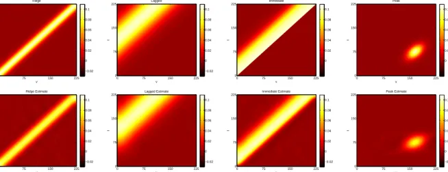
We select true surfaces to mimic biologically plausible time varying associations. The top row of Figure 1.1 contains the heat maps of each surface. Each surface represents a different type of association, equations for which can be found in the Appendix. The
ridge surface represents a relationship where the strongest association betweenx(v)and
y(t) occurs along the line v = t. In other words, changes in y(t) are associated with
concurrent changes in x(v). The lagged surface suggests a relationship where changes
inx(v) at a given time are associated with later changes in y(t), but the strongest effect
is delayed. The relationship between x(v) and y(t) in the immediate surface is similar
to that in the lagged, however the strongest effect occurs immediately before dying off.
Finally, the peak scenario demonstrates a setting where changes iny(t)at a given time are
associated with later changes inx(v)and the association is characterized by a single peak.
For each surface, we generate 200 simulated data sets and draw posterior samples using a burn-in of 1000 followed by a chain of 1000 samples. We use Daubechies wavelets with four vanishing moments and three levels of decomposition. In preliminary simulations, zero-padding reduced edge effects better than symmetric-half point padding. Thus we implement zero-padding for all models. Motivated by the ERP data structure, we set the total number of time points in both time domains to be 225. For the wPC decomposition,
we keep components accounting for 99.0% of the variability inXW. Averaged posterior
estimates for each surface are found in the bottom row of Figure 1.1. Results from all
three sample sizes were similar, thus we only present simulations for n = 25, N = 50
here. Results forn = 100, N = 200 can be found in the Appendix. For each dataset we
v t Ridge 225 150 75 0 225 150 75 0 −0.02 0 0.02 0.04 0.06 0.08 0.1 v t Lagged 225 150 75 0 225 150 75 0 −0.02 0 0.02 0.04 0.06 0.08 0.1 v t Immediate 225 150 75 0 225 150 75 0 0 0.02 0.04 0.06 0.08 0.1 v t Peak 225 150 75 0 225 150 75 0 0 0.02 0.04 0.06 0.08 0.1 v t Ridge Estimate 225 150 75 0 225 150 75 0 −0.02 0 0.02 0.04 0.06 0.08 0.1 v t Lagged Estimate 225 150 75 0 225 150 75 0 −0.02 0 0.02 0.04 0.06 0.08 0.1 v t Immediate Estimate 225 150 75 0 225 150 75 0 −0.02 0 0.02 0.04 0.06 0.08 0.1 v t Peak Estimate 225 150 75 0 225 150 75 0 −0.02 0 0.02 0.04 0.06 0.08 0.1
Figure 1.1: Heat maps of the true surfaces for simulation study are in the top row. The bottom row
contains estimated surfaces for each simulated scenario based on a sample size ofn= 25with two
measure per subject,Ci = 2∀i, for a total ofN = 50observations. Each surface is the average of
the posterior estimate for the true surface based on 200 simulated datasets.
We also examine the performance of the BFDR, SimBaS, and GBPV procedures in
simu-lation using a global αof 0.05. For the BFDR, we use a δ-intensity change of 0.05 which
is roughly half the max signal from each surface. For comparison, we also generate un-adjusted PWCIs. To evaluate the three procedures, we calculate false discovery rate, sen-sitivity, experiment-wise error rate (EWER), and type I error. Define false discovery rate,
FDR, as the number of flagged locations(v, t)with true value ≤ divided by the total
number of flagged locations. Next define the sensitivity, SENΥ, as the number of flagged
locations (v, t) with true magnitude> Υ divided by the total number of locations with
true magnitude > Υ. EWER is calculated as the proportion of simulated datasets with
at least one falsely discovered location, i.e. a flagged location with true value≤ . Type
I error is calculated using a null simulation with true surface β(v, t) = 0 ∀v ∈ V, t ∈ T
and determining the proportion of simulated datasets with at least one location flagged as significant.
Figure 1.1 allows for direct comparison of each estimated surface to the truth. For all surfaces, we see the model performed quite well, effectively reconstructing all the true surfaces. Estimation improves as sample size increases. Not surprisingly, rMSE decreases
as sample size increases though even the smallest sample size produced small rMSEs.
Heat maps containing the averaged set of flagged coefficients, ψ, for the BFDR and the
average SimBa scores across datasets can be found in the Appendix. Both procedures correctly identified regions of elevated association in all four surfaces.
Table 1.1 displays both the average false discovery rate, FDR, and the average sensitivity,
SENΥ, for each scenario using = 0.01,0.05 and Υ = 0.05,0.075. For each procedure,
we use α = 0.05 to select the set of flagged coefficients. We can see that the BFDR and
SimBaS procedures performs similarly well by both measures, though BFDR does better
for a higherandΥ. While the PWCI has very good sensitivity, it comes at the cost of an
inflated false discovery rate. EWER is calculated using = 0.01. Additionally, SimBaS
controls experiment-wise type I error quite well at 0.05. While BFDR has a slightly low
type I error of 0.04, PWCI has a very high value of 0.645. To assessPGBP V we determine
the percent of datasets under each scenario with PGBP V < 0.05. In each scenario, all
datasets havePGBP V <0.05.
These simulation results suggest our method performs well both in estimation and in inference. Even at the smallest sample size we considered, for this signal to noise ratio the model effectively reproduces the true surface. Both the BFDR and SimBaS capture the strongest regions of association without spuriously flagging too many non-significant coefficients. They also control well for type I error. Further, BFDR and SimBaS outper-form the PWCI while maintaining reasonable sensitivity. Increasing sample size improves these facets of the model. Additional results, not included here nor in the Appendix, are available upon request.
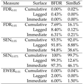
Table 1.1: FDR, sensitivity, experiment-wise error rate (EWER), and type I error values by inference
procedure. The BFDR use aδintensity change of0.05. To determine assessment values for SimBaS,
a cutoff of α = 0.05 was used. Likewise, the PWCI used 95% point-wise credible intervals to
determine significant locations.
Measure Surface BFDR SimBaS PWCI
FDR0.01 Lagged 0.06% 0.08% 5.80% Peak 0.48% 0.75% 22.9% Ridge 0.12% 0.19% 20.5% Immediate 2.25% 2.80% 20.9% FDR0.05 Lagged 5.74% 13.9% 44.7% Peak 4.01% 20.4% 73.5% Ridge 9.75% 15.6% 53.3% Immediate 5.74% 7.58% 38.1% SEN0.05 Lagged 98.1% 96.2% 99.9% Peak 64.9% 73.4% 99.9% Ridge 96.8% 93.4% 99.9% Immediate 97.9% 93.8% 99.9% SEN0.075 Lagged 99.9% 99.3% 100% Peak 94.4% 88.2% 99.9% Ridge 99.8% 97.6% 99.9% Immediate 99.9% 96.2% 99.9% EWER0.01 Lagged 7.00% 16.5% 100% Peak 4.50% 10.5% 100% Ridge 9.50% 49.0% 100% Immediate 100% 100% 100%
1.5
Application
1.5.1
Description of ERP Data Set
To demonstrate the features of the proposed model, we analyze data from the Department of Behavioral Sciences at the University of Texas M. D. Anderson Cancer Center. As part of a smoking cessation trial, researchers obtained Event Related Potentials (ERPs) at baseline for subjects viewing a series of images of different types, including neutral, emotional (positive and negative), and cigarette-related.
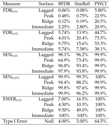
EEG was continuously recorded during image presentation and collected using a 129-channel Geodesic Sensor Net and amplified with AC-coupled high-input impedance (200
MΩ) amplifier (Geodesic EEG System 250; Electrical Geodesics, Inc., Eugene, OR)
refer-enced to the Cz electrode. The time series were preprocessed as described in Versace et al. (2010a), with 0.1Hz high pass and 100Hz low pass filters, blink-corrected using spatial filtering, transformed to average reference, segmented into 900ms segments from 100ms before each image shown to 800ms after, obvious artifacts removed, and ERPs averaged across images for each image type per subject/electrode. After this processing, for each subject, we are left with functions of length 225 for each image type for all 129 electrodes. Example curves recorded from 180 participants at electrode Cz (#129, in the middle of the crown of the head) during presentation of cigarette-related and neutral images can be seen in Figure 1.2 with the average over curves included in red. Curves under the other image-types are similar in appearance. The irregularity and localized spikiness of the raw curves motivates our use of wavelets in our modeling approach (Figure 1.2).
While many analyses are of interest for these data, in this paper we aim to characterize the time-varying relationship between ERP output from pairs of electrodes, focusing on two pairs in particular. The first pair is 55 and 129. Electrode 129, as previously mentioned, is positioned at the top of the head and electrode 55 is located directly behind it. We
−100 100 300 500 700 −10 −5 0 5 10 15 Sensor 129: Cigarette potential ( µ V) time (ms) −100 100 300 500 700 −5 0 5 10 15 20 25 30 Sensor 129: Neutral potential ( µ V) time (ms)
Figure 1.2: On the left, raw profile curves are plotted in gray with the mean in red from electrode 129 under the cigarette image condition. On the right, are raw curves and the mean from electrode 129 under the neutral image condition.
axis. The second pair is 75 and 11. Electrode 75 is an occipital electrode located at the back of the head while electrode 11 is at the front. Output from these two electrodes is expected to exhibit a negative correlation and thus we anticipate a negative association along the diagonal axis. For each pair of electrodes, we jointly model the association between the electrodes under both the neutral and cigarette image conditions resulting in a multilevel data structure. Thus for each model, subjects have four curves resulting from measurements from two electrodes while viewing two different image types.
1.5.2
Analysis
We fit two models to the data. In general, the model is given by
yicg(t) = 1(g = 0) α0(t) + Z v∈V xic0(v)β0(v, t)dv (1.9) + 1(g = 1) α1(t) + Z v∈V xic1(v)β1(v, t)dv +Ui(t) +Eic(t), (1.10)
whereg denotes group membership, 0 for neutral, 1 for cigarette. For the first model we
used Electrode 129 as the outcome function and Electrode 55 as the predictor function and for the second we used Electrode 11 as the outcome and Electrode 75 as the predictor.
In both models, inference was drawn on both image-specific surfaces,β0 and β1, as well
as the difference surfaceD(v, t) = β1(v, t)−β0(v, t). As in the simulation study, we used
Daubechies wavelets with four vanishing moments and three levels of decomposition along with zero-padding. Prior to decomposition, we standardized both outcome and predictor functions by time. After DWT, the dimensions of the transformed functional
outcomes from Electrodes 129 and 11 were both 360×245. After wPC, the dimensions
of the transformed functional predictors were360×72for Electrode 55 and360×62for
Electrode 75. We obtained 1000 posterior samples from the MCMC after a burn in of 1000. Spot checks of the trace plots of key parameters suggested MCMC convergence.
We considered inference for both models using all three procedures. For the BFDR
proce-dure, we selected a globalαof 0.05 when implementing BFDR on the difference surfaces.
We choose a somewhat strict intensity change of δ = 0.05 to focus on large differences
between the surfaces. We also implemented BFDR on the image-specific surfaces in both
models. There theα-level was reduced to 0.025 for each surface, however the intensity
change, δ, remained at 0.05 so to only flag relatively large associations. Using the same
intensity change for both models allows us to compare the two. For the PWCI, we also
usedα = 0.05.
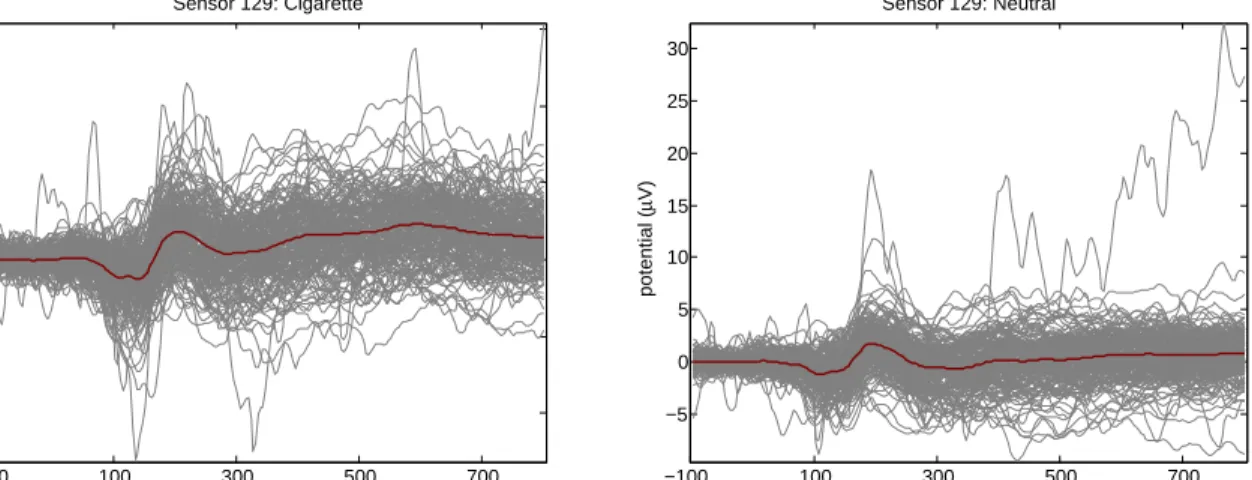
Figure 1.3 contains posterior means of all three surfaces for both models. Examination of the posterior estimates of the difference surfaces found in the first column of Figure 1.3 suggest little to no systematic difference between image type in both models. When we look at the image-specific surfaces in the model using electrodes 129 and 55 (top row,
sec-ond and third column, Figure 1.3), we see an elevated ridge of association along thet=v
diagonal, which is the relationship we anticipated between these two adjacent electrodes. Note that this relationship is strongest in the first 300 ms in the ERP or 200 ms post picture
presentation (image presentation occurred att =v = 0), which corresponds to the initial
response to viewing the image. Transitioning to the image-specific surfaces of the model using electrodes 11 and 75 (bottom row, second and third column, Figure 1.3), we see a
v t Difference Surface −100 100 300 500 700 700 500 300 100 −100 −0.1 −0.05 0 0.05 0.1 0.15 v t Neutral Surface −100 100 300 500 700 700 500 300 100 −100 −0.1 −0.05 0 0.05 0.1 0.15 0.2 v t Cigarette Surface −100 100 300 500 700 700 500 300 100 −100 −0.1 −0.05 0 0.05 0.1 0.15 0.2 v t Difference Surface −100 100 300 500 700 700 500 300 100 −100 −0.1 −0.05 0 0.05 0.1 0.15 v t Neutral Surface −100 100 300 500 700 700 500 300 100 −100 −0.1 −0.05 0 0.05 0.1 0.15 0.2 v t Cigarette Surface −100 100 300 500 700 700 500 300 100 −100 −0.1 −0.05 0 0.05 0.1 0.15 0.2
Figure 1.3: The top row contains surface estimates for the association between electrodes 129 and 55. Posterior surfaces comparing electrodes 11 to 75 are in the second row. The estimated posterior surface of the difference between cigarette and neutral is found in the first column. Group specific surface estimates are in the second and third columns, Neutral and Cigarette respectively. ERP output from electrode 129 is the response and the output from electrode 55 is the predictor for the first model and electrode 75 is the predictor of electrode 11 in the second model.
v t P(|D(v,t)| < 0.05) −100 100 300 500 700 700 500 300 100 −100 0 0.2 0.4 0.6 0.8 1 v t P(|β0(v,t)| < 0.05) −100 100 300 500 700 700 500 300 100 −100 0 0.2 0.4 0.6 0.8 1 v t P(|β1(v,t)| < 0.05) −100 100 300 500 700 700 500 300 100 −100 0 0.2 0.4 0.6 0.8 1 v t P(|D(v,t)| < 0.05) −100 100 300 500 700 700 500 300 100 −100 0 0.2 0.4 0.6 0.8 1 v t P(|β0(v,t)| < 0.05) −100 100 300 500 700 700 500 300 100 −100 0 0.2 0.4 0.6 0.8 1 v t P(|β1(v,t)| < 0.05) −100 100 300 500 700 700 500 300 100 −100 0 0.2 0.4 0.6 0.8 1
Figure 1.4: Heat maps containing the posterior probabilities from the BFDR procedure usingaδ
intensity change of 0.05. Coefficients in white have a high probability of being greater thanδand
thus likely to be included inψ, the set of coefficients flagged as significant. Black coefficients have
a low probability of being greater thanδand are thus less likely to be flagged as significant. The
top row contains results from the model using electrodes 129 and 55 while the second row contains results from the model using electrodes 75 and 11.
200 ms to 300 ms past presentation. Once again, this is consistent with the expected rela-tionship between these two electrodes.
Figure 1.4 contains results from the BFDR procedure on the difference surface for both
models. Each heat map plots the posterior probabilitiesPBF DR. We see that for both
mod-els, most locations have a low probability of being greater thanδ. In fact, plottingψ, we
see no significantly flagged regions (see the Appendix), suggesting there is little evidence that the correlation across the two electrodes differs across image types. The second and third columns of Figure 1.4 show the application of the BFDR to the image-specific
sur-faces in each model, and again the heat maps plot the posterior probabilitiesPBF DR. We
see that the probabilities along the ridge are quite large suggesting that ridge of positive association is significant up until almost 300 ms past image presentation. However the negative association along the ridge we saw in the second model has lower probabilities
v
t
Difference SimBa Scores
−100 100 300 500 700 700 500 300 100 −100 0.001 0.01 0.05 0.1 0.25 0.5 v t
Neutral SimBa Scores
−100 100 300 500 700 700 500 300 100 −100 0.001 0.01 0.05 0.1 0.25 0.5 v t
Cigarette SimBa Scores
−100 100 300 500 700 700 500 300 100 −100 0.001 0.01 0.05 0.1 0.25 0.5 v t
Difference SimBa Scores
−100 100 300 500 700 700 500 300 100 −100 0.001 0.01 0.05 0.1 0.25 0.5 v t
Neutral SimBa Scores
−100 100 300 500 700 700 500 300 100 −100 0.001 0.01 0.05 0.1 0.25 0.5 v t
Cigarette SimBa Scores
−100 100 300 500 700 700 500 300 100 −100 0.001 0.01 0.05 0.1 0.25 0.5
Figure 1.5: Heat maps containing the SimBa scores for each surface of both models. The top row contains results from the model using electrodes 129 and 55 while the second row contains results
from the model using electrodes 75 and 11. Scores are plotted on thelog-scale with the color axis
on the exponential scale. White regions represent coefficients with low SimBa scores, black regions represent coefficients with high SimBa scores.
along the ridge at theδ = 0.05cut-off. Heat maps of the regions flagged as significant by
the procedure are also found in the Appendix.
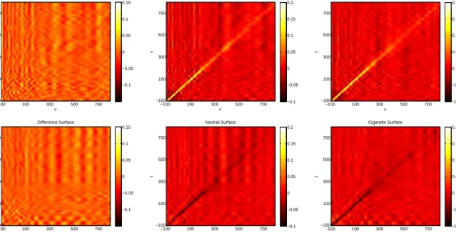
For the SimBaS procedure, we plot heat maps of the logged SimBa Scores in Figure 1.5. We see that for both difference surfaces, the SimBa scores are all relatively large (at least
0.5 or more), and the global Bayesian p-value for both isPD
GBP V = 0.5, suggesting there
is not enough evidence to conclude differences in the coefficient surfaces between image types. The second and third columns of Figure 1.5 show the SimBaS procedure applied to the image-specific surfaces. These heat maps are also plotted on the log-scale so to distinguish variations in small SimBa scores. For both models, we see evidence of a
non-zero coefficient surface for each image type (PGBP V0 =PGBP V1 = 0.001for the model using
Electrodes 129 and 55,PGBP V0 = 0.001andPGBP V1 = 0.005for the model using Electrodes
11 and 75). Additionally, the SimBaS procedure detects the ridge of positive association in first model but only finds some of the negative associations in second.
Heat maps of flagged significant locations using PWCI can be found in the Appendix. Not surprisingly, the PWCI is more sensitive to minor variations in the surface where there ap-pears to be no systematic association. While both BFDR and SimBaS found no significant locations in the difference surfaces, the PWCI flags a number of regions and also finds a
number of significant locations in the image-specific surfaces that are off thet = v axis
while suggesting the association lingers longer. Given the results in the simulation stud-ies, we interpret these results cautiously, as they may likely be spurious, and feel more confident in the multiplicity-adjusted inference from the BFDR and SimBaS procedures.
1.6
Discussion
Functional data analysis is an expanding field requiring more work to fill in gaps in the literature and build upon the general knowledge of the field. Previous work on function regression is limited. Here we present a general approach to function-on-function regression modeling which benefits from several attributes. First, our approach
can use any basis function for y(t) and x(v) allowing us to handle functions of
vari-ous types, including those with spiky and smooth features, and allowing us to parsi-moniously model correlated residuals rather than assuming iid errors. Second, we get fully Bayesian inferences on all model quantities including point-wise credible intervals, posterior probabilities interpretable as Bayesian FDRs, joint credible intervals, and Sim-BaS that provide global and experiment-wise inferential quantities. Further generation of posterior predictive distributions is straightforward, so, for example, functional dis-criminant analysis can be performed (Zhu, Brown, and Morris, 2012). Third, our infer-ence procedures correctly identify regions of elevated association without falsely flag-ging too many non-significant coefficients. Fourth, our method resides within the func-tional mixed model (FMM) framework as put-forth by Morris and Carroll (2006) that handles correlation between functions and random effects through random effect func-tion distribufunc-tion, and thus accounting for the various sources of variability in multi-level
models. Finally, the FMM framework also allows any combination of continuous and discrete scalar predictors, functional predictors, and their interactions, allowing function-on-function regression to be done in a much broader modeling context.
We demonstrated by simulation that our model performs well for realistic sample sizes and forms of functional association with fits improving as sample size increases. Simu-lations also show the BFDR and SimBaS procedures have better false discovery and type I error rates than the PWCI with comparable sensitivity. Our approaches for global in-ference and multiple-testing adjustment for Bayesian inin-ference using BFDR, SimBaS, and GBPV are of general interest and can be used in other functional regression settings. Our application displays the ability of the model to estimate the forms of the relationship of ERP output between different electrodes on the scalp. With the neighboring electrodes,
a positive association was expected and seen along the diagonal axist =v while a
nega-tive association was expected and seen between electrodes on opposite sides of the scalp. Further, both our inference procedures were able to detect these associations as signifi-cant, even the one based on experiment wise error rate.
In summary, the function-on-function mixed model with basis-space modeling com-prises a flexible approach to the function-on-function regression setting. The method performed well in both simulation and application. Further studies are needed to explore the model’s performance in more complex settings, including non-functional components beyond a factor variable, incorporating multiple functional predictors, and various types of random effect correlation structures. Additionally, further examination of data reduc-tion techniques could improve the modeling prowess of the method.
Acknowledgements
This work was supported by grants from the National Institutes of Health (ES007142, ES000002, ES016454, CA134294, CA160736, CA016672, DA032581).
References
Brumback, B. A., and Rice, J. A. (1998). Smoothing spline models for the analysis of nested
and crossed samples of curves.Journal of the American Statistical Association93, 398–408.
Cardot, H., Ferraty, F., and Sarda, P. (1999). Functional linear model.Statistics & Probability
Letters45,11–22.
Chen, K. and M ¨uller, H. G. (2012). Modeling Repeated Functional Observations.Journal
of the American Statistical Soceity107,1599–1609.
Cinciripini, P. M., Robinson, J. D., Karam-Hage, M., Minnix, J. A., Lam, C. Y., Versace, F., Brown, V. L., Engelmann, J. M., and Wetter, D. W. (2013). The effects of varenicline and bupropion-SR plus intensive counseling on prolonged abstinence from smoking,
depression, negative affect, and other symptoms of nicotine withdrawal.JAMA
Psychi-atry,70,522–533.
Gertheiss, J., Maity, A., and Staicu, A.-M. (2013). Variable Selection in Generalized
Func-tional Linear Models.Stat2,86–101.
Goldsmith, J., Bobb, J., Crainiceanu, C. M., Caffo, B., and Reich, D. (2011). Penalized
Functional Regression.Journal of Computational and Graphical Statistics20,830–851.
Goldsmith, J., Greven, S., and Crainiceanu, C. M. (2013). Corrected Confidence Bands for
Functional Data Using Principal Components.Biometrics69,41–51.