Dissertations
2020
Model estimation, identification and inference for next-generation
Model estimation, identification and inference for next-generation
functional data and spatial data
functional data and spatial data
Shan Yu
Iowa State University
Follow this and additional works at: https://lib.dr.iastate.edu/etd
Recommended Citation Recommended Citation
Yu, Shan, "Model estimation, identification and inference for next-generation functional data and spatial data" (2020). Graduate Theses and Dissertations. 18251.
https://lib.dr.iastate.edu/etd/18251
This Dissertation is brought to you for free and open access by the Iowa State University Capstones, Theses and Dissertations at Iowa State University Digital Repository. It has been accepted for inclusion in Graduate Theses and Dissertations by an authorized administrator of Iowa State University Digital Repository. For more information, please contact [email protected].
by
Shan Yu
A dissertation submitted to the graduate faculty in partial fulfillment of the requirements for the degree of
DOCTOR OF PHILOSOPHY
Major: Statistics
Program of Study Committee: Dan Nettlteton, Co-major Professor
Lily Wang, Co-major Professor Peng Liu
Yumou Qiu Zhengyuan Zhu
The student author, whose presentation of the scholarship herein was approved by the program of study committee, is solely responsible for the content of this dissertation. The Graduate College will ensure this
dissertation is globally accessible and will not permit alterations after a degree is conferred.
Iowa State University Ames, Iowa
2020
TABLE OF CONTENTS
Page
LIST OF TABLES . . . v
LIST OF FIGURES . . . vii
ACKNOWLEDGMENTS . . . x
ABSTRACT . . . xi
CHAPTER 1. GENERAL INTRODUCTION . . . 1
CHAPTER 2. ESTIMATION AND INFERENCE FOR GENERALIZED GEOADDITIVE MODELS 5 2.1 Abstract . . . 5
2.2 Introduction . . . 6
2.3 Methodology . . . 9
2.3.1 Model Setup . . . 9
2.3.2 Spline Approximation . . . 10
2.3.3 Penalized Quasi-likelihood Estimators . . . 11
2.4 Two-Stage Estimator and Simultaneous Confidence Band . . . 14
2.5 Implementation . . . 16 2.5.1 First Stage . . . 16 2.5.2 Second Stage . . . 18 2.6 Simulation . . . 19 2.6.1 Example 1 . . . 19 2.6.2 Example 2 . . . 24
2.7 Application to Crash Data . . . 27
2.7.1 Domain of Interest . . . 27
2.7.2 Analysis and Findings . . . 30
2.8 Concluding Remarks . . . 34
2.9 References . . . 35
2.10 Appendix A. Theoretical Results with Details . . . 39
2.10.1 Notations and Assumptions . . . 39
2.10.2 Properties of Penalized Quasi-likelihood Estimators . . . 42
2.10.3 Properties of Local Polynomial Estimators . . . 53
2.11 Appendix B. Implementation for the Bivariate spline . . . 65
2.11.1 An example ofΨ . . . 65
CHAPTER 3. MULTIVARIATE SPLINE ESTIMATION AND INFERENCE FOR
IMAGE-ON-SCALAR REGRESSION . . . 69
3.1 Abstract . . . 69
3.2 Introduction . . . 70
3.3 Models and Estimation Method . . . 73
3.3.1 Image-on-scalar Regression Model . . . 73
3.3.2 Spline Approximation over Triangulations and Penalized Regression . . . 74
3.4 Variance Function Estimation and Simultaneous Confidence Corridors . . . 76
3.4.1 Estimation of the Variance Function . . . 76
3.4.2 Bootstrap Simultaneous Confidence Corridors (SCCs) . . . 78
3.5 Implementation . . . 79
3.5.1 Asymptotic Properties of the BPST Estimators . . . 80
3.5.2 Piecewise Constant Spline over Triangulation Smoothing . . . 82
3.6 Simulation Studies . . . 84
3.6.1 Example 1 . . . 84
3.6.2 Example 2 . . . 86
3.7 ADNI Data Analysis . . . 88
3.8 Conclusion . . . 91
3.9 References . . . 92
3.10 Appendix A. Theoretical Results with Details . . . 95
3.10.1 Properties of Bivariate Splines . . . 96
3.10.2 Uniform Convergence of the Unpenalized Spline Estimators . . . 102
3.10.3 Asymptotic Properties of Penalized Spline Estimators . . . 106
3.10.4 Asymptotic Properties of Piecewise Constant Spline Estimators . . . 114
3.10.5 Convergence of the Covariance Estimator . . . 119
3.11 Appendix B. Additional Simulation and Application Results . . . 128
3.11.1 More Results of Simulation Studies . . . 128
3.11.2 Additional ADNI Data Analysis Results . . . 129
CHAPTER 4. SPARSE MODELING OF FUNCTIONAL LINEAR REGRESSION VIA FUSED LASSO WITH APPLICATION TO GENOTYPE-BY-ENVIRONMENT INTERACTION STUD-IES . . . 140
4.1 Abstract . . . 140
4.2 Introduction . . . 141
4.3 Methodology . . . 143
4.3.1 Functional Linear Models with Heterogeneous Coefficient Functions . . . 143
4.3.2 Spline Approximation . . . 143
4.3.3 Functional Linear Regression with Fused Penalty . . . 144
4.3.4 Graph-constrained Adaptive Fused Lasso . . . 145
4.4 Implementation . . . 146
4.4.1 The ADMM Algorithm . . . 147
4.4.2 Weights for Adaptive Fused Lasso . . . 150
4.4.3 Knots Selection . . . 151
4.5 Asymptotics . . . 152
4.5.1 Notations and Assumptions . . . 152
4.5.3 Adaptive Fused Lasso Estimator . . . 155 4.6 Simulation Study . . . 156 4.6.1 Simulation Study 1 . . . 158 4.6.2 Simulation Study 2 . . . 160 4.7 Application . . . 161 4.7.1 Data . . . 164
4.7.2 Growing Degree Day Time Scale . . . 165
4.7.3 Data Analysis . . . 165
4.8 Discussion . . . 168
4.9 References . . . 168
4.10 Appendix A. Theoretical Results with Details . . . 170
4.10.1 Additional Notations . . . 170
4.10.2 Some Basic Lemmas . . . 171
4.10.3 Proof of Theorem4.1 . . . 175
4.10.4 Proof of Theorem4.2 . . . 177
4.11 Appendix B. Additional Simulation Results . . . 183
CHAPTER 5. GENERAL CONCLUSION . . . 188
LIST OF TABLES
Page
Table 2.1 MISE of the functional component estimators and 10-fold cross-validated MSPE. . 22
Table 2.2 The coverage rate of the 95% SCBs for univariate functions. . . 22
Table 2.3 The MISE of the estimators of the component functions and the coverage rate of the 95% SCB for the univariate functions. . . 27
Table 2.4 Covariates used in the crash dataset and their correspondingp-value. . . 30
Table 2.5 Estimation and prediction results. . . 34
Table 3.1 Estimation errors of the coefficient estimators,σ= 2.0. . . 86
Table 3.2 Estimation errors of the coefficient function estimators,σ= 1.0. . . 88
Table 3.3 The coverage rate of the95%SCCs for the coefficient functions. . . 88
Table 3.4 10-fold CV results for the ADNI dataset. (×10−2) . . . 91
Table 3.5 Estimation errors of the coefficient estimators,σ= 1.0. . . 131
Table 3.6 Estimation errors of the coefficient function estimators,σ= 0.5. . . 132
Table 3.7 Estimation errors of the coefficient function estimators in the 35th slice. . . 132
Table 3.8 The coverage rate of the95%SCCs for the coefficient functions defined over the 35th slice. . . 133
Table 3.9 Distribution of patients by diagnosis status and gender. . . 134
Table 4.1 Description of the methods used in the simulation studies. . . 157
Table 4.2 Clustering results of the intercepts and coefficient functions in simulation study 1. . 159
Table 4.3 RMISEs (RMSEs) of the coefficient functions (intercepts) and the average com-puting time in Simulation Example 1. . . 184
Table 4.5 RMISEs (RMSEs) of the coefficient functions (intercepts) in simulation study 2. . . 186 Table 4.6 Cluster size of the intercept terms. . . 187
LIST OF FIGURES
Page
Figure 1.1 An example of PET imaging data. . . 3
Figure 2.1 Tampa-St. Petersburg urbanized area and its census block groups . . . 7
Figure 2.2 The true univariate component functions in Example 1. . . 20
Figure 2.3 Triangulations on the horseshoe domain. . . 21
Figure 2.4 Plots ofβk(xk)(dotted curve), the SBL estimator (solid curve) and the 95% SCBs (grey bands),k= 1,2,3, based onn= 2,000observations. . . 23
Figure 2.5 Contour maps for the true bivariate function and its estimators. . . 24
Figure 2.6 Boxplots of the MISEs of the estimators of functional components in Case I using different combinations of knots and triangulations. . . 25
Figure 2.7 Boxplots of the MISEs of the estimators of functional components in Case II using different combinations of knots and triangulations. . . 26
Figure 2.8 Plots of the true function (dashed line), its SBL estimator (black curve) and the 95% SCB (grey band). . . 28
Figure 2.9 Plots of the estimatedα(·)(left plot) and the trueα(·)(right plot). . . 29
Figure 2.10 (a) Triangulation of Tampa-St. Petersburg urbanized area; (b) estimatedα(·)with cities labeled. . . 31
Figure 2.11 Plots of the SBL estimate (solid line), the 95% SCB (grey band) and the zero line (dashed line). . . 32
Figure 2.12 Histgram of the deviance residuals . . . 34
Figure 2.13 A simple triangulation with two triangles. . . 65
Figure 3.1 A schematic diagram of proposed modeling approach. . . 71
Figure 3.3 The true coefficient functions in the Simulation Example 1. . . 85 Figure 3.4 The BPST estimate and significance map of the coefficient functions for the5th
slice of the PET images. The yellow and blue color in the significance map in-dicates the regions that zero is below the lower SCC or above the upper SCC, respectively. . . 90 Figure 3.5 Triangulations for the horseshoe domain. . . 129 Figure 3.6 True coefficient functions and their different estimators for Case I in Example 1. . . 129 Figure 3.7 True coefficient functions and their different estimators for Case II in Example 1. . 130 Figure 3.8 Triangulations for the 5th slice (43, 44) and 35th slice (45, 46) of the brain
image in Simulation Example 2. . . 130 Figure 3.9 True coefficient functions and their estimators and 95% SCCs based on the 5th slice.133 Figure 3.10 True coefficient functions and their estimators and 95% SCCs based on the 35th
slice. . . 134 Figure 3.11 Triangulation sets used in the ADNI data analysis. . . 135 Figure 3.12 The BPST estimates of the coefficient functions for the ADNI data based on the
8th, 15th and 35th slices, respectively. . . 136 Figure 3.13 The BPST estimates of the coefficient functions for the ADNI data based on the
55th, 62nd and 65th slices, respectively. . . 137 Figure 3.14 The “significance” map (based on the 95% SCC) for the coefficient functions for
the ADNI data. The yellow color and blue color on the map indicate the regions that zero is below the lower SCC or above the upper SCC, respectively. . . 138 Figure 3.15 The “significance” map (based on the 95% SCC) for the coefficient functions for
the ADNI data. The yellow color and blue color on the map indicate the regions that zero is below the lower SCC or above the upper SCC, respectively. . . 139 Figure 4.1 The graphs for group identification with color representing true group structures. . 161 Figure 4.2 Plots of the true coefficient functions in simulation studies 1 and 2. . . 162 Figure 4.3 Solution path of lasso (the tuning parameter for coefficient function is λ1 = 1)
and adaptive lasso (the tuning parameter for coefficient function is λ1 = 1) in simulation study 2 withnk = 50andσ= 1.0. λ0 = 1andλ0 = 10−4are selected tuning parameters, respectively. . . 163
Figure 4.4 Solution path of lasso in simulation study 2 withnk = 50andσ = 1.0, when the
tuning parameter for intercepts isλ0 = 1.λ1= 1.93is the selected tuning parameter.163
Figure 4.5 Solution path of adaptive lasso in simulation study 2 withnk = 50andσ = 1.0, when the tuning parameter for intercepts isλ0 = 10−4. λ1 = 1.93is the selected
tuning parameter. . . 164 Figure 4.6 Estimated clusters for intercepts and coefficient functions. Each circle point
repre-sents one hybrid, and we use different colors to distinguish different clusters. . . 166 Figure 4.7 Estimated coefficient functions with 95% bootstrap confidence intervals in the
ap-plication study. The dashed blue line is a horizontal line at zero. The solid blue line is the vertical line at time point one, representing the anthesis date. . . 167 Figure 4.8 Estimations results based on differentτ’s in the simulation study 1. . . 183 Figure 4.9 Estimations results based on differentN’s in the simulation study 1. . . 183
ACKNOWLEDGMENTS
I want to take this opportunity to express my thanks to all those who have kindly helped me with various aspects of conducting research and pursuing my doctoral degree.
First and foremost, I wish to express my deepest gratitude to my advisors, Dr. Dan Nettleton and Dr. Li Wang, for being such incredible mentors. Their enthusiasm for research always influences me. I would like to thank Dr. Nettleton for providing me the opportunity to work as a research assistant for the Plant Science Institute and inspiring me in both researching and teaching. Dr. Wang’s passion, intelligence, and diligence to research significantly inspired me and strengthened my faith to continue my career in academics. I learnt a lot from her both in non-parametric statistics and how to be a good researcher.
I would additionally like to thank Dr. Zhengyuan Zhu for his guidance throughout all the stages of my graduate career. I am grateful to my committee members: Dr. Peng Liu and Dr. Yumou Qiu, for their exper-tise, insight and help on my dissertation research. I want to thank the faculty in the Statistics Department at Iowa State University for encouraging a collaborative environment and creating such a lovely department. It is an invaluable experience for me to study in the department.
Last but not least, I would like to acknowledge my family for being great support through my journey, pursuing a Ph.D. degree. My special thank goes to my friends for their loving encouragement during my graduate life.
ABSTRACT
This dissertation is composed of three research projects focused on model estimation, identification, and inference for next-generation functional data and spatial data.
The first project deals with data that are collected on a count or binary response with spatial covariate information. In this project, we introduce a new class of generalized geoadditive models (GGAMs) for spatial data distributed over complex domains. Through a link function, the proposed GGAM assumes that the mean of the discrete response variable depends on additive univariate functions of explanatory variables and a bivariate function to adjust for the spatial effect. We propose a two-stage approach for estimating and making inferences of the components in the GGAM. In the first stage, the univariate components and the geographical component in the model are approximated via univariate polynomial splines and bivariate penalized splines over triangulation, respectively. In the second stage, local polynomial smoothing is applied to the cleaned univariate data to average out the variation of the first-stage estimators. We investigate the consistency of the proposed estimators and the asymptotic normality of the univariate components. We also establish the simultaneous confidence band for each of the univariate components. The performance of the proposed method is evaluated by two simulation studies and the crash counts data in the Tampa-St. Petersburg urbanized area in Florida.
In the second project, motivated by recent work of analyzing data in the biomedical imaging studies, we consider a class of image-on-scalar regression models for imaging responses and scalar predictors. We propose to use flexible multivariate splines over triangulations to handle the irregular domain of the objects of interest on the images and other characteristics of images. The proposed estimators of the coefficient functions are proved to be root-nconsistent and asymptotically normal under some regularity conditions. We also provide a consistent and computationally efficient estimator of the covariance function. Asymptotic pointwise confidence intervals (PCIs) and data-driven simultaneous confidence corridors (SCCs) for the coefficient functions are constructed. A highly efficient and scalable estimation algorithm is developed.
Monte Carlo simulation studies are conducted to examine the finite-sample performance of the proposed method. The proposed method is applied to the spatially normalized Positron Emission Tomography (PET) data of Alzheimer’s Disease Neuroimaging Initiative (ADNI).
In the third project, we propose a heterogeneous functional linear model to simultaneously estimate multiple coefficient functions and identify groups, such that coefficient functions are identical within groups and distinct across groups. By borrowing information from relevant subgroups, our method enhances esti-mation efficiency while preserving heterogeneity. We use an adaptive fused lasso penalty to shrink subgroup coefficients to shared common values within each group. We also establish the theoretical properties of our adaptive fused lasso estimators. To enhance the computation efficiency and incorporate neighborhood in-formation, we propose to use a graph-constrained adaptive lasso. A highly efficient and scalable estimation algorithm is developed. Monte Carlo simulation studies are conducted to examine the finite-sample perfor-mance of the proposed method. The proposed method is applied to a dataset of hybrid maize grain yields from the Genomes to Fields consortium.
CHAPTER 1. GENERAL INTRODUCTION
This dissertation is mainly focused on developing novel, flexible and reliable statistical methodologies, as well as practical and efficient data analysis tools for solving problems arising from data science. These statistical methodologies and computation algorithms have important applications in many areas, such as urbanization studies, precision medicine, remote sensing, economics, computer science, climatology, and environmental studies.
The wide availability of data observed over time and space, in particular through inexpensive geograph-ical information systems, has stimulated many studies in a variety of disciplines, including environmental science, epidemiology, political science, transportation and economics. Spatial or spatiotemporal data are generated at varying scales and levels of complexity. Complex data demand statistical models that are suffi-ciently flexible to adapt to underlying signals, allowing scientists to discover unexpected patterns and predict the time evolution of the variables of interest. To deal with such complex data, some big challenges fac-ing statisticians are (1) many practical data exhibit clearly heterogeneous and non-stationary features, such as spatial heterogeneity due to topographic differences and various land cover types. (2) The observations distribute unevenly over an irregular domain. (3) The size of spatiotemporal data can be very large. Many spatiotemporal data sets (e.g., high resolution remote sensing data) include millions of observations per day. These challenges motivate us to search and study flexible and computational efficient non-/semi-parametric models for spatiotemporal analysis methods.
In Chapter 2, we introduce a new class of generalized geoadditive models (GGAMs) for spatial data distributed over complex domains. To motivate the study, consider the analysis of road traffic crashes, which have been one of the major sources of fatalities and injuries in the United States. Count data models are often used to identify factors significant to crash frequencies, where the influence of demographical and socioeconomic conditions on the crash occurrence and spatial patterns of crashes can assist decision-makers in implementing appropriate road safety management actions. In this project, we use univariate
spline functions to capture the effects of demographical and socioeconomic conditions on the number of car crashes, and we use a bivariate spline function to adjust for spatial effects. Also, to average out the variation of the spline estimators and to access the uncertainty of our proposed estimators, we apply local polynomial smoothing in the second stage. We investigate the consistency of the proposed estimators and the asymptotic normality of the univariate components. We also establish the simultaneous confidence band for each of the univariate components.
With the rapid growth of modern technology, many large-scale gene-environment-wide association stud-ies and biomedical imaging studstud-ies have been, are being, and will be conducted to collect massive datasets with high resolution, such as 1D curves (e.g., medical monitoring data from wearable medical devices) and multi-modality imaging, thus boosting the investigation of next generation functional data. Functional data analysis (FDA) methods allow sophisticated interpretation of shape information and play a critical role in exploiting the output of high-resolution data with complex structure. Although FDA research has gained widespread popularity in recent years, enhancing the capability of next generation FDA remains a long-standing challenge. In Chapters 3and4, we develop a sequence of flexible and reliable models for functional data.
In Chapter 3, we focus on the study of imaging data. In recent years there has been explosive growth in the number of imaging studies in medical and public health research. It is of great interest for people to understand how subject-level characteristics, including clinic variables and genetic factors, would influence imaging phenotypes. For example, Figure1.1shows spatially normalized Positron Emission Tomography (PET) imaging data of people at different cognitive stages: Alzheimer’s Disease (AD), mild cognitive im-pairment (MCI), and cognitive normal (CN). In this example, it is of great interest to figure out the influence of disease status on the PET imaging phenotypes. To analyze such data, we face two main challenges: (1) the effects of explanatory variables on the imaging data vary over the locations; (2) there are spatial correlations among the pixels within each image.
Motivated by the above challenges, in Chapter 3, we propose to use multivariate splines for image on scalar regression, which can capture the varying association between imaging phenotypes with a set of
explanatory variables, and we use functional principal component techniques to explicitly incorporate the spatial correlation structure of imaging data.
Figure 1.1 An example of PET imaging data.
For biomedical imaging data, objects (e.g., organs) on images are usually expected to be irregularly shaped. Many smoothing methods, such as kernel smoothing, tensor product smoothing, and wavelet smoothing, suffer from the problem of “leakage” across complex domains. Next, imaging data often have different visual qualities. There is a great demand for development of flexible estimation methods of vari-ous smoothness to adaptively smooth biomedical imaging data. In the second project, we tackle the above challenges by using bivariate splines defined on triangulations, which is an effective tool to handle data distributed on irregular regions with complex boundaries. By investigating theoretical properties of the es-timated functions, we derive the asymptotic normality of the coefficient functions and use it as a guidance to construct pointwise confidence intervals and simultaneous confidence corridors, which are an important tool to identify the effective regions, and quantify the variability of the functional components.
In Chapter 4, we consider a functional linear model with application to genotype-by-environment in-teraction studies. Understanding genotype-by-environment inin-teraction is essential to the development of breeding strategies, which seek to customize genotypes to the characteristics of particular environments. Some genotypes may respond similarly to one or more environmental factors. Grouping genotypes ac-cording to their responses to environmental characteristics is of scientific interest and is useful for
obtain-ing efficient estimators. Motivated by maize yield data, which contains 1,008 genotypes along with daily recorded weather data throughout the growing period, we consider a heterogeneous functional linear re-gression model. In this model, we assume that the coefficient functions for time-indexed environmental variables are genotype-dependent and can be partitioned into unknown groups, where coefficient functions are identical for genotypes in the same group but different across groups. The motivation of this paper is to estimate heterogeneous functional linear regression and automatically identify the underlying grouping structure.
Fusion learning has drawn a lot of attention as an increasing number of data sources have become easily available in this big data era. It strategically combines information to improve estimation efficiency while preserving parameter heterogeneity. In the third project, we propose a fusion learning method for a heterogeneous functional linear model.
We use univariate spline approximation to estimate the coefficient functions and use the adaptive lasso to perform shrinkage estimation. This approach is appealing for several reasons. First, we can use spline functions to approximate the coefficient functions and incorporate structural constraints on the coefficient functions through their spline coefficients. Second, adaptive lasso is a convex penalty that facilities efficient numerical optimization using convex optimization methods. We use an alternating direction method of multipliers (ADMM) algorithm in our optimization procedure.
In addition to considering a pairwise fused penalty, we implement a graph-constrained adaptive lasso, which not only reduces the computation burden but also incorporates prior information about the underlying clustering structure. The constrained lasso has wide applications in the literature. We apply graph-constrained adaptive lasso in our model fitting, where each genotype is treated as a node, graph edges are determined by genetic similarity, and the edges determine which pairwise differences in estimation are penalized.
CHAPTER 2. ESTIMATION AND INFERENCE FOR GENERALIZED GEOADDITIVE MODELS
Shan Yu1, Guannan Wang2, Li Wang1, Chenhui Liu3and Lijian Yang4
1Department of Statistics, Iowa State University, Ames, IA
2Department of Mathematics, College of William & Mary, Williamsburg, VA 3Turner-Fairbank Highway Research Center, Federal Highway Administration, McLean, VA 4Center for Statistical Science and Department of Industrial Engineering, Tsinghua University, China
Modified from a manuscript published inJournal of the American Statistical Association
2.1 Abstract
In many application areas, data are collected on a count or binary response with spatial covariate in-formation. In this paper, we introduce a new class of generalized geoadditive models (GGAMs) for spatial data distributed over complex domains. Through a link function, the proposed GGAM assumes that the mean of the discrete response variable depends on additive univariate functions of explanatory variables and a bivariate function to adjust for the spatial effect. We propose a two-stage approach for estimating and making inferences of the components in the GGAM. In the first stage, the univariate components and the geographical component in the model are approximated via univariate polynomial splines and bivariate pe-nalized splines over triangulation, respectively. In the second stage, local polynomial smoothing is applied to the cleaned univariate data to average out the variation of the first-stage estimators. We investigate the consistency of the proposed estimators and the asymptotic normality of the univariate components. We also establish the simultaneous confidence band for each of the univariate components. The performance of the proposed method is evaluated by two simulation studies. We apply the proposed method to analyze the crash counts data in the Tampa-St. Petersburg urbanized area in Florida.
2.2 Introduction
Regression methods are commonly used in statistics to examine associations between the response and the set of explanatory variables. When the relationship between the variables is complex and can not be easily modeled by specific linear or non-linear functions, a generalized additive model (GAM) provides a flexible regression relationship. GAMs were first introduced byHastie and Tibshirani(1987,1990), which assume that the mean of the discrete response variable depends on an additive set of predictors through a link function. Since then GAMs have been widely used in many areas. The focus of this work is on GAM for spatial data randomly distributed over a particular geographical region.
To motivate the study, consider the analysis of road traffic crashes, which have been one of the major sources of fatalities and injuries in the United States. Count data models are often used to identify factors significant to crash frequencies, where the influence of demographical and socioeconomic conditions on the crash occurrence and spatial patterns of crashes can assist decision-makers in implementing appropriate road safety management actions (Miaou et al.,2003;Liu and Sharma,2017,2018). Figure2.1(a) shows the Tampa-St. Petersburg urbanized area in Florida, which is consisted of 1,761 census block groups. A census block group is a geographical unit with homogeneous population characteristics, economic status, and living conditions for the population survey. Rural areas were excluded from this study, as their population densities often drop to nearly zero, thus it is not meaningful to analyze their crash data. The frequency of crashes off the state highway system within each census block group in the year of 2014 were collected from the Florida Department of Transportation; see Figure 2.1 (b). In addition, explanatory variables, including vehicle-miles traveled, demographic and commuting variables, were collected from the Florida Department of Transportation and U.S. Census Bureau, and many of them exhibit pronounced non-linear relationships with the response variable.
To analyze such kind of data, researchers face at least three main challenges. First of all, traditional regression methods often assume the data are distributed on a regular sampling grid over a rectangular domain, however, in this study and many other similar cases in spatial studies, observations are dense at some locations while sparse at others, and the shape of the domains is complicated or even shows gaps and holes; seeRamsay(2002) andWood et al.(2008). Conventional smoothing tools suffer from the problem
Off Crashes <5 5 − 10 10 − 15 15 − 30 >30 (a) Tampa-St. Petersburg urbanized area (b) Crashes within individual census block group
Figure 2.1 Tampa-St. Petersburg urbanized area and its census block groups
of “leakage” across the complex domains, which refers to the poor estimation over difficult regions by smoothing inappropriately across boundary features, such as peninsulas. The second challenge is how to adjust for the spatial effect and provide measures of the nonlinear effect of covariates and assess the impact of uncertainty. In general, inference for GAM for spatial data is underdeveloped and often made based on
ad hocmethods with little understanding of the statistical properties. Last but not least, the computational issue usually is a big challenge for spatial data analysis, as the sample size tends to be large due to the development of remote sensing technology and automated sensor networks. Thus, there is a great need of methodology that is practical, computationally efficient and theoretically reliable.
To address the above-mentioned challenges, in this paper we introduce a class of generalized geoadditive models (GGAMs), a synthesis of geostatistics and GAMs, for spatial data randomly distributed over irregular domains. We aim at developing the corresponding estimation and inference procedure for the GGAMs. In the literature, there are two main streams of spatial regression modeling approaches to include spatial information into the model. The first approach adds spatial weights or spatial correlation into a regression modeling, for example, the spatial autoregressive (SAR) model or conditional autoregressive (CAR) model (Lee,2004;Zhu et al.,2010). The second approach is based on some smoothing techniques, for example, kernel, wavelet or spline smoothingRamsay(2002) use a deterministic smooth surface function to describe
the variations and connections among values at different locations.Kammann and Wand(2003) combine the kriging method with the penalized spline regression, and suggest a mixed model representation for model fitting. In our paper, we take the second approach, where the effect of explanatory variables are modeled with additive univariate functions and the spatial effect is modeled via a bivariate function.
In the proposed GGAM, when the spatial component is ignored, the model becomes the traditional GAM since all the components left in the model are univariate functions. There have been a number of proposals for fitting the GAMs, for instance, the spline method of Stone (1986), Xue and Liang(2010) andWang et al.(2011); the kernel method ofYu et al.(2008),Yang et al. (2003) andLiang et al.(2008); and the two-stage methods ofHorowitz et al. (2004),Wang and Yang (2007) and Liu et al.(2013). For estimating bivariate functions defined over rectangular domains, there are several popular smoothing tools: kernel, wavelet, bivariate P-splines (Marx and Eilers, 2005) and thin plate splines (Wood,2003). In the past three decades, there has been a great interest in developing the smoothing techniques which can handle irregular domains with complex boundaries; see, for example, Ramsay(2002);Wang and Ranalli(2007); Wood et al. (2008); Sangalli et al. (2013); Lai and Wang (2013); Miller and Wood (2014); Wang et al. (2018). In this paper, we approximate the bivariate function of the spatial effect using the bivariate splines (smooth piecewise polynomial functions over a triangulation of the domain of interest) over triangulations inLai and Schumaker(2007). We prefer the bivariate penalized splines (BPS) due to their (i) convenient representations with flexible degrees and various smoothness, (ii) computational efficiency, and (iii) great ability of handling the sparse designs.
Although the above-mentioned spline smoothing seems to be incredibly useful, it provides only conver-gence rates of the estimators but no asymptotic distributions unless we assume the errors are iid gaussian, so it is difficult to assign any measure of confidence to the estimators. The simultaneous confidence bands (SCB) is a powerful tool to evaluate and visualize the variability of the estimators and to make global in-ferences; seeWang and Yang(2009),Krivobokova et al.(2010),McKeague and Zhao(2006),Wiesenfarth et al. (2012) and Zheng et al. (2016) for some related theory and applications of SCBs. To develop the SCBs for each individual component function of the explanatory variables in GGAMs, we propose a one-step spline backfitted local polynomial estimator, referred to as the SBL estimator. In the first stage, we use
spline smoothers to approximate the univariate additive components and the geographical component. In the second stage, local polynomial smoothing is then applied to the cleaned univariate data to average out the variation of the first-stage estimators and obtain SCBs.
Under some regularity conditions, we obtain the asymptotically normal distribution of the SBL estima-tors and establish the SCBs for the functions of the covariates. Our approach merges the advantages of three smoothing methods (polynomial spline, bivariate spline and local polynomial) that balance each other out. It enables the spline smoothing to act as an efficient pilot, quickly guiding the fitting towards good solutions. In addition, it allows us to keep the asymptotically normal distribution of the local polynomial estimator, without its computational burden. Furthermore, it properly accounts for all covariate information and spa-tially improves the estimation accuracy. The entire fitting and inference procedure can be implemented easily and efficiently using standard methodology and software.
The rest of the paper is structured as follows. In Section 2.3, we describe our model, then we give a brief review of univariate splines and bivariate splines over triangulations and introduce the penalized quasi-likelihood estimation method. Section 2.4provides the SCBs for the functions of the covariates. Section 2.5introduces how to implement the proposed procedure in practice. In Section2.6, we conduct simulation studies to evaluate the finite sample performance of the proposed method. Section2.7illustrates our method using a real dataset. Some concluding remarks are given in Section2.8. Proofs and other technical details are given in the Appendices A and B.
2.3 Methodology 2.3.1 Model Setup
In the following, let Si = (Si1, Si2)> be the location ofith point,i = 1, . . . , n, which ranges over a
bounded domainΩ⊆R2 of arbitrary shape, for example, a domain with polygon boundary. LetYi be the
response variable andXi= (Xi1, . . . , Xip)>be the explanatory variables at locationSi.
We assume the conditional density of Y given (X,S) = (x,s) belongs to the exponential family
fY|X,S(y|x,s) = exp [yξ(x,s)− B {ξ(x,s)}+C(y)], for known functionsBandC, whereξ is the
B0{ξ(x,s)}.In this paper,µ(x,s)is modeled via a link functiongin the following additive form of un-known univariate smooth functionsβ= (β1, . . . , βp)>and an unknown bivariate smooth functionα(·):
g{µ(x,s)}=
p
X
k=1
βk(xk) +α(s). (2.1)
If Var (Y|X=x,S=s) = σ2V {µ(x,s)} for some known positive functionV, then estimation of the mean can be achieved by replacing the conditional log-likelihood functionlog{fY|X,S(y|x,s)}with a
quasi-likelihood function`(ϑ, y), which satisfies∇ϑ`(ϑ, y) = σ2yV−(ϑ)ϑ .Our estimation method is based on
a nonparametric quasi-likelihood approach as described below.
2.3.2 Spline Approximation
In the first stage, we approximate each of the univariate additive components in the model via uni-variate polynomial splines. The geographical component is approximated using biuni-variate penalized splines over triangulation, which is proved to be efficient to deal with data distributed on irregular domains with complicated boundaries. Below we start with a brief review of univariate splines and bivariate splines.
2.3.2.1 Univariate polynomial spline approximation
Suppose the covariate Xk is distributed on a compact interval [ak, bk], k = 1, . . . , p. We
approxi-mate the univariate components {βk(·)}pk=1 in (2.1) by polynomial splines for their simplicity in
com-putation. For any k = 1, . . . , p, let υk be a partition of [ak, bk] with Jn interior knots, where υk =
{ak=υk,0< υk,1<· · ·< υk,Jn < υk,Jn+1 =bk}. The polynomial splines of order%+ 1are polynomial
functions with%-degree (or less) on intervals[υkj, υk,j+1),j= 0, . . . , Jn−1,and[υk,Jn, υk,Jn+1], and have
%−1continuous derivatives globally. LetUk =Uk%([ak, bk], υk)be the space of such polynomial splines,
andU0
k ={u ∈ Uk : Eu(Xk) = 0}. This ensures that the spline functions are centered; seeXue and Yang
(2006),Wang and Yang(2007) andWang et al.(2014).
2.3.2.2 Bivariate spline over triangulation
In this paper we consider the spatial domainΩis a polygon of arbitrary shape, which can be partitioned into finitely many triangles. According to Lai and Schumaker (2007), a collection 4 = {τ1, ..., τN} of
N triangles is called a triangulation ofΩ = ∪N
i=1τi provided that if any nonempty intersection between a
pair of triangles in4is either a shared vertex or a shared edge. Given a triangleτ ∈ 4, let Rτ be the
radius of the largest disk contained in τ, and let|τ|be length of the the longest edge. Define the shape parameter ofτ as the ratioπτ =|τ|/Rτ. Note that whenπτ is small, the triangles are relatively uniform in
the sense that all angles of triangles in the triangulation4are relatively the same. Denote the size of4by |4|:= max{|τ|, τ ∈ 4}.
For a triangle with non-zero areaτ ∈ 4and any fixed pointv∈R2, letb
1,b2andb3be the barycentric
coordinates of vrelative toτ. The Bernstein basis polynomials of degree d ≥ 1relative to triangle τ is defined asBijkτ,d(v) = i!j!k!d bi
1b j
2bk3, i+j +k = d. For any integerd ≥ 1 and triangle τ, let Pd(τ) be
the space of all polynomials of degree less than or equal todon τ. Then, any polynomialζ ∈ Pd(τ)can be written asζ|τ = Pi+j+k=dγijkτ Bijkτ,d,where the coefficients γτ = {γijkτ , i+j+k = d}are called
B-coefficients ofζ.
For any integer r ≥ 0, let Cr(Ω) be the collection of all rth continuously differentiable functions over Ω. Given a triangulation 4, we define the spline space of degree dand smoothness r over 4as Srd(4) = {ζ ∈ Cr(Ω) : ζ|τ ∈ Pd(τ), τ ∈ 4}. Let{Bm}m∈M be the set of bivariate Bernstein basis polynomials forSrd(4), whereMis an index set of|M| =N(d+ 1)(d+ 2)/2basis functions. Then we
can represent any functionζ ∈Srd(4)using the following basis expansion:
ζ(s) = X
m∈M
Bm(s)γm=B(s)>γ, (2.2) where γ> = (γm, m ∈ M) is the spline coefficient vector. For smooth join between two polynomials
on adjoining triangles, we need to impose some linear constraints on the spline coefficientsγ in (2.2). To be more specific, we assume thatγsatisfiesΨγ = 0, whereΨis the matrix that collects the smoothness conditions across all the shared edges of triangles. An example ofΨis given in2.11.1. The above bivariate spline basis can be easily constructed via the R packageBPST(Wang et al.,2019).
2.3.3 Penalized Quasi-likelihood Estimators
In data-sparse regions, penalized splines provide a more convenient tool for data fitting than the un-penalized splines. As discussed inLai and Wang (2013), the number of triangles for bivariate penalized
smoothing is not essential when the number is above some minimum depending upon the degree of the splines. Another advantage is that when we have regions of sparse data, BPS can be considered as a direct ridge regression or shrinkage type method which can alleviate multicollinearity issue. Thus, to reduce com-plexity in triangulation selection and enhance the performance of bivariate splines in data fitting, we exploit the BPS in the quasi-likelihood of the model below.
To define the penalized spline method, for any direction sj, j = 1,2, let ∇qsjf(s) be the qth order derivative in the directionsj at the points= (s1, s2). Let
E(f) = Z Ω (∇2s 1f) 2+ 2(∇ s1∇s2f) 2+ (∇2 s2f) 2 ds 1ds2. (2.3)
To fit the GGAM, we seek a bivariate function α(·) and univariate functions ofβk(·), k = 1, . . . , p, that
maximize the following penalized quasi-likelihood function:
n X i=1 ` " g−1 ( p X k=1 βk(Xik) +α(Si) ) , Yi # −λ 2E(α). (2.4)
Directly solving this penalized maximization is challenging since it involves unstructured nonparametric functions which are subject to the “curse of dimensionality”. To overcome this difficulty, we consider some smoothing method. Under some suitable smoothness conditions,βk’s andαcan be well approximated by
the univariate spline basis functions and the Bernstein basis polynomials introduced in Sections2.3.2.1and 2.3.2.2, respectively.
Letukj(xk),j∈ J be the original B-spline basis functions for thekth covariate, whereJ is the index
set of the basis functions. Letu0kj(xk) = ukj(xk)−
Eukj(Xk) Euk1(Xk)uk1(xk), Ukj(xk) = u0 kj(xk) SD{u0 kj(Xk)}, j ∈ J, then EUkj(Xk) = 0 andEUkj2 (Xk) = 1. Suppose the nonlinear component can be well approximated by a spline function so that, for all xk ∈ [ak, bk],βk(xk) ≈ Pj=1Jn+%+1θkjUkj(xk) = U>k(xk)θk, where
Uk(xk) = (Uk1(xk), . . . , Uk,Jn+%+1(xk)) >
andθk = (θk1, . . . , θk,Jn+%+1)
>
is a vector of coefficients. Let Sn×2 ={(Si1, Si2)}ni=1 be the location design matrix andXn×p ={(Xi1, . . . , Xip)}ni=1 be the collection
of all covariates. Fori = 1, . . . , n, let B>i = {Bm(Si), m ∈ M}, and denoteB = (B1, . . . ,Bn)> the n× |M|evaluation matrix of Bernstein basis polynomials. Then maximizing the penalized quasi-likelihood function in (2.4) is equivalent to minimizing
− n X i=1 ` " g−1 ( p X k=1 Uk(Xik)>θk+B(Si)>γ ) , Yi # +1 2λγ >Pγ subject to Ψγ=0, (2.5)
wherePis the block diagonal penalty matrix satisfying thatγ>Pγ =E(Bγ). See Section2.11.2for the formula used to constructP. It is worth noting that according to the Assumption (A3), the optimization problem in (2.5) has a unique solution.
To solve the constrained minimization problem (2.5), we first remove the constraint via the following QR decomposition: Ψ> = QR = (Q1Q2) RR12
, whereQis an orthogonal matrix andR1 is an upper
triangle matrix, the submatrixQ1is the firstr(ris the rank of matrixΨ) columns ofQ, andR2is a matrix
of zeros. We reparametrize usingγ =Q2γ∗ for someγ∗, then it is guaranteed thatΨγ=0. The problem
(2.5) is now converted to a conventional penalized minimization problem without any restriction:
LP(θ,γ∗) =− n X i=1 ` " g−1 ( p X k=1 Uk(Xik)>θk+B(Si)>Q2γ∗ ) , Yi # +λ 2γ ∗>Q> 2PQ2γ∗. (2.6)
For practitioners, the construction ofPandQ2 can be carried out via the R packageBPST (Wang et al.,
2019).
Letbθ andγb
∗
be the minimizer of (2.6), i.e. (θb,γb
∗
) = arg minLP(θ,γ∗), then, the univariate spline estimator ofβk(xk)and bivariate spline estimator ofα(s)are
b βk(xk) =Uk(xk)>bθk, b α(s) =B(s)>γb = X m∈M Bm(s)bγm,
where the estimated spline coefficients areγb ={bγm, m∈ M}
>=Q
2bγ
∗ .
We first establish theL2convergence rate of the spline estimatorsβbk(xk)and b
α(s). For any Lebesgue measurable functionψ(u)on a domainD, for example,D= [ak, bk]orΩ⊆R2, letkψk2L2 =RDψ2(u)du andH=Jn−1.
Theorem2.1. Under Assumptions (A1)–(A6) in Appendix A, the spline estimatorsβbk(xk)andαb(s)satisfy that p X k=1 kβbk−βkkL2+kαb−αkL2 =Oa.s. ( (H−1/2+|4|−1) logn n 1/2 +H%+1+|4|d+1+ λ n|4|4 ) .
2.4 Two-Stage Estimator and Simultaneous Confidence Band
It is very difficult to derive the asymptotic distribution for the spline estimators introduced in Section 2.3, so no measures of confidence can be assigned to these estimators. To represent the uncertainty in the estimate of the nonlinear effect of the covariates, we propose the SCB forβk’s via the backfitting method
using spline estimators obtained in Section2.3as pilot followed by local polynomial estimators.
The basic idea is that for everyk= 1, . . . , p, we estimate thekth additive functionβk(·)in model (2.1)
nonparametrically by assuming that other nonparametric components {βk0(·) : k0 6= k} are known. The
problem turns into a univariate function estimation problem. DenoteK a continuous kernel function, and let Kh(u) = K(u/h)/hbe a rescaling ofK, whereh is usually called the bandwidth. This leads to an
“oracle” smootherβbkoofβk, where
{βbko(xk),βbko0(xk)} = arg max a0,a1 n X i=1 ` g −1 a0+a1(Xi,k −xk) +α(Si) + p X k06=k βk0(Xik0) , Yi Khk(Xik−xk).
Asymptotic properties of smoothers ofβbko(xk)can be easily established based on these assumptions. We
sayx∈χk = [ak, bk]is a boundary point if and only ifx=ak+chkorx=bk−chkfor some0≤c <1
and an interior point otherwise. Letχhk be the interior of the supportχk. Letν2 =
R
u2K(u)duandf
k
be the probability density function ofXk. Forj = 1,2, letρj(x) =
dg−1(x)/dx j.
σ2V(g−1(x)) =
{g0(g−1(x))}jσ2V(g−1(x))−1
.For the quasi-likelihood function`{g−1(x), y}, letq1(x, y) = ∂x∂`{g−1(x), y} and q2(x, y) = ∂
2
∂x2`{g−1(x), y}. It is clear that q1(x, y) = {y −g−1(x)}ρ1(x) andq2(x, y) = {y− g−1(x)}ρ01(x) −ρ2(x) hold. Let C(K) = R K0(u)2du/R K(u)2du, ah =
p
−2 log(h), and for any
α∈(0,1), denote the quantile
Qh(α) =ah+a−h1[log{pC(K)/2π} −log{−log√1−α}].
Theorem 2.2 below shows the pointwise and uniform asymptotically normality of the “oracle” estimator
b
βo
Theorem2.2. Suppose Assumptions (A1)–(A4) and (A7) in Appendix A hold. Then, for anyk= 1, . . . , p, xk ∈ χhk, ifnh 5 k=O(1), we have, asn→ ∞, σn,k−1(xk) b βok(xk)−βk(xk)− βk00(xk) 2 ν2h 2 k →N(0,1),
and if Assumptions (A1)–(A4), (A7) and (A8) (ii) are satisfied, then
lim n→∞P ( sup xk∈χhk σn,k−1(xk)|βbko(xk)−βk(xk)| ≤Qhk(α) ) = 1−α, whereσ2n,k(xk) =n−1hk−1Eρ2{Pp k=1βk(Xk) +α(S)}|Xk=xk −1 fk(xk)−1R K2(u)du.
Since the true functionsβk’s andα are unknown, we replace those with the pilot estimatorsβbk andαb
obtained in Section2.3and apply the above backfitting idea to obtain the spline-backfitted local polynomial (SBL) estimator {βbkSBL(xk),βbSBL 0 k (xk)} = arg max a0,a1 n X i=1 ` g −1 a0+a1(Xi,k −xk) +αb(Si) + p X k06=k b βk0(Xik0) , Yi Khk(Xik−xk).
Theorem 2.3. Under Assumptions (A1)–(A5), (A6’), (A7) and (A8) (i) in Appendix A, the SBL estimator satisfies
sup
xk∈χhk
|βbkSBL(xk)−βbko(xk)|=Oa.s.(n−1/2logn), sup
xk∈χhk hk|βbSBL 0 k (xk)−βbo 0 k(xk)|=Oa.s.(n−1/2logn).
The proofs of Theorems 2.2 and 2.3 are given in the Section 2.10. Theorem 2.3 implies that the difference between the SBL estimator and the “oracle” estimator is negligible compared to the difference between the “oracle” estimatorβbko(xk)and the true functionβk(xk), that is, the SBL estimatorβbkSBL(xk)is
oracle-efficient. Consequently, the SBL estimator inherits the same asymptotic normality (both pointwise and uniform asymptotically normality) from the “oracle” estimator, as stated in Corollary2.1below, which follows directly from Theorems2.2and2.3, thus, the proof is omitted.
Corollary2.1. Under Assumptions (A1)–(A5), (A6’), (A7) and (A8) (i) in Appendix A, for anyxk ∈ χhk,
we have, asn→ ∞, σ−n,k1(xk) n b βkSBL(xk)−βk(xk)−β00k(xk)ν2h2k/2 o →N(0,1).
If Assumptions (A1)–(A5), (A6’), (A7) and (A8) (ii) are satisfied, then, for anyα∈(0,1)andk= 1, . . . , p, lim n→∞P ( sup xk∈χhk σn,k−1(xk)|βbkSBL(xk)−βk(xk)| ≤Qhk(α) ) = 1−α.
Corollary2.1yields the following100(1−α)%SCB forβk(xk):
b
βkSBL(xk)±σn,k(xk)Qhk(α), xk∈χhk. (2.7)
2.5 Implementation 2.5.1 First Stage
Let Y = (Y1, . . . , Yn)> be the vector of n observations of the response variable. Denote Ui =
U1(Xi1)>,· · · ,Up(Xip)>
>
andU = (U1,· · · ,Un)>. We use the following iteratively re-weighted
least square (IRLS) to minimize the objective function in (2.6), which leads to enormous reductions in com-putational complexity. LetG(k),V(k) andρ(k)2 be diagonal matrices with elementsg0(µ(k)i ),V(µ(k)i )and
ρ2(µ(k)i ), respectively. At the(k+ 1)th iteration, we consider the following objective function:
R(k+1)= {V (k)}−1/2{Y−µ(θ,γ∗)} 2 +λ 2γ ∗>Q> 2PQ2γ∗,
whereµ(θ,γ∗) = g−1(U>θ+B>Q2γ∗), and it can be approximated by its first order Taylor expansion
around(θ(k),γ∗(k)): µ(θ,γ∗)≈µ(k)−J(k) ( θ γ∗ − θ(k) γ∗(k) ) withµ(k) =µ(θ(k),γ∗(k)) ={µ(k)
i }>1≤i≤nandJ(k) ={G(k)}−1(U BQ2)being the “Jacobian” matrix.
Therefore, R(k+1) ≈ {V(k)}−1/2 " Y−µ(k)−J(k) ( θ γ∗ − θ(k) γ∗(k) )# 2 +λ 2γ ∗>Q> 2PQ2γ∗. Then, we have R(k+1)≈ {V (k)}−1/2{G(k)}−1hG(k)(Y−µ(k)) +η(k)−U>θ−B>Q 2γ∗ i 2 +λ 2γ ∗>Q> 2PQ2γ∗ = (ρ (k) 2 ) 1/2( e Y(k)−U>θ−B>Q2γ∗) 2 +λ 2γ ∗> Q>2PQ2γ∗, (2.8)
where η(k) = (η1(k), . . . , ηn(k))> with ηi(k) = Ui>θ(k) +B>i Q2γ∗(k), Ye(k) = (Ye (k) 1 , . . . ,Ye (k) n )> with e Yi(k)=g0(µi(k))(Yi−µ(k)i )+η (k)
i . By minimizing (2.8) with respect to(θ,γ∗), we obtain(θ(k+1),γ∗(k+1)).
Notice that to start the iteration, we only needµ(0)andη(0), not(θ(0),γ∗(0)), which simplifies the procedure of choosing initial value. In the Poisson case, we setµ(0)i =yi+ 0.01andη(0)i =g(µ
(0) i ).
Knots selection. For univariate spline smoothing, we suggest placing knots on a grid of evenly spaced sample quantiles. Assumption (A6) in Appendix A suggests that the number of knotsJnneeds to satisfy:
n1/(2%+2)(logn)−1/(2%+2) Jn n2/5, where% ≥1 is the degree of the polynomial spline basis
func-tions. The widely used quadratic/cubic splines both satisfy this condition. In practice we suggest taking the following rule-of-thumb number of interior knots: Jn = min{bc1n1/(2%+2)c,bn/(4p)c}+ 1, wherec1 is a tuning parameter (typically,c1 ∈ [1,5]), and the termn/(4p) is to guarantee that there are at least four
observations in each subinterval between two adjacent knots to avoid getting (near) singular design matrices in smoothing.
Triangulation selection. An optimal triangulation is a partition of the domain which is best according to some criterion that measures the shape, size or number of triangles. For example, a “good” triangulation usually refers to those with well-shaped triangles, no small angles or/and no obtuse angles. Other criteria include the density control (adaptivity) and optimal size (number of triangles), etc. For a fixed number of triangles,Lai and Schumaker (2007) andLindgren et al.(2011) recommend selecting the triangulation according to “max-min” criterion which maximizes the minimum angle of all the angles of the triangles in the triangulation. Monte Carlo experiments in our simulation studies show that there must be enough triangles to capture the features of the surface, but once this minimum necessary number of triangles has been reached, further increasing the number of triangles usually has little effect on the fitting process. Therefore, one needs to make certain that the triangulation is sufficiently fine to capture the feature in the dataset and not so large that computational burden is unnecessarily heavy. In practice, if the boundary of the spatial domain is not too complicated, we suggest taking the number of triangles as the following: Nn =
min{bc2n1/(d+1)c, n/4}+ 1,for some tuning parameterc2 (typically,c2 ∈ [1,20]). However, when the spatial domain does look complicated,Nncan be set (much) larger than nso that the domain can be very
OnceNnis chosen, one can build the triangulated meshes using typical triangulation construction methods
such as Delaunay Triangulation.
Roughness penalty selection. The roughness penalty parameter λ can be selected using data-driven approaches, for example, the generalized cross-validation (GCV) (Craven and Wahba,1979;Wahba,1990) is such a criterion and is widely used for choosing the penalty parameter. Letbρ2be the diagonal matrix with
elementsρ2(µib), and
C(λ) = U>bρ2U U>bρ2BQ2 Q>2B>bρ2U Q>2(B>ρb2B+λP)Q2 .
Denote the smoothing or hat matrix asS(λ) = (U BQ2)C(λ)−1(U BQ2)>ρb2. LetYe = (Ye1, . . . ,Yen)
>
withYie =g0(bµi)(Yi−µib) +ηib. We minimize the following
GCV(λ) = nkbρ
1/2
2 {Ye −S(λ)Y}ke 2
{n−tr(S(λ))}2
over a grid of values to selectλ.
2.5.2 Second Stage
The performance of the SBL estimator is also dependent upon the bandwidth selection and other esti-mators of the parameters.
Bandwidth selection. Note that Assumption (A8) in Appendix A requires that the bandwidths in the backfitting are of order aroundn−1/5. Thus, the bandwidth selection can be done using a standard routine in the literature, see discussions inFan et al.(1995) andFan and Gijbels(1996). By minimizing the asymptotic mean integrated squared errors (AMISE), we can obtain the optimal bandwidth
hk,AMISE =n−1/5CK1/5 R ρ2,k(xk)dxk R βk00(xk)2fk(xk)dxk 1/5 , where ρ2,k(xk) = E ρ2{Ppk=1βk(Xk) +α(S)}|Xk =xk
. The optimal bandwidth could be approxi-mated by n−1/5CK1/5 " n−1Pn i=1{ρb2,k(Xik)} −1 b fk−1(Xik) n−1Pn i=1βbk00(Xik)2 #1/5 ,
wherefbkis estimated by kernel density estimation,βbk00is obtained from the spline estimatorβbkandρb2,k(Xik) is an estimator ofρ2,k(Xik). Let b σ2 = 1 n n X i=1 {Yi−g−1(ηbi)} 2/V(g−1( b ηi)), b ρ2,k(xk) =n−1 n X i=1 (g0(g−1(ηib))) 2 b σ2V(g−1(bηi)) −1 Kh(Xik−xk)
with a rule-of-the-thumb bandwidthh. To construct pointwise confidence intervals or SCBs of the univariate functions, we suggest takinghk=hk,AMISE(logn)−1/4to satisfy the requirement of Assumption (A8).
Estimating σn,k(xk). For any k = 1, . . . , p, we obtain the estimator of σn,k(xk) by σbn,k(xk) =
n−1/2h−k1/2ρb −1 2,k(xk)fbk−1(xk) R K2(u)du. 2.6 Simulation
In this section, we conduct two simulation studies to evaluate the finite sample performance of the proposed method.
2.6.1 Example 1
We consider a modified horseshoe domain in Sangalli et al.(2013) and randomly samplen = 1,000 and2,000locations on the domain. The response variable Yi is generated from Poisson distribution and
negative binomial distribution with log link functions as described in the following two cases.
Case I: Poisson distribution:Yi ∼Poisson(µi), wherelog(µi) =P3
k=1βk(Xik)+α(Si), i= 1, . . . , n.
Case II: Negative binomial distribution: Yi ∼ NB(θ, µi/(θ+µi)), whereθ = 5 andlog(µi)is the
same as Case I andE(Yi) =µiand Var(Yi) =µi+µ2i/θ.
We conduct1000Monte Carlo replications. In each replication,Xi1,Xi2 andXi3 are uniformly
gen-erated from [0,1], andSi is uniformly generated from the horseshoe domain, and Xi1, Xi2 andXi3 and
Si are independent of each other. The true univariate functions β1(x),β2(x),β3(x)are illustrated in
Fig-ure2.2(a)–(c), respectively, whereβ1(x) = 1/2 sin(2πx)−cos(πx)−E{1/2 sin(2πX1)−cos(πX1)}, β2(x) = 4(x−0.5)2−E{4(X2−0.5)2}andβ3(x) =x−E(X3). Figure2.5(a) shows the contour map of
the true bivariate functionα(·), which is modified based on a similar function given inWood et al.(2008) andSangalli et al.(2013).
0.0 0.2 0.4 0.6 0.8 1.0 − 1.0 − 0.5 0.0 0.5 1.0 m3 0.0 0.2 0.4 0.6 0.8 1.0 − 0.4 0.0 0.4 m3 0.0 0.2 0.4 0.6 0.8 1.0 − 0.4 0.0 0.2 0.4 m3 (a)β1 (b)β2 (c)β3
Figure 2.2 The true univariate component functions in Example 1.
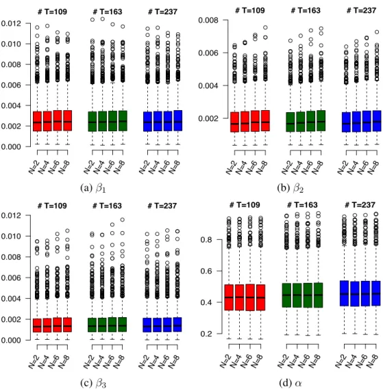
To implement the proposed procedure, one needs to select the knots for a univariate spline, the triangu-lation for a bivariate spline, the bandwidth for the local linear method, as well as the smoothness penalty parameter. We have conducted extensive simulations to examine whether and how sensitive the choice of knots, triangulation and bandwidth on the performance of the proposed method. For all the univariate splines, we use cubic B-splines with the number of interior knots Jn = 2,4,6,8 equally spaced on the
sample quantiles. For the bivariate spline smoothing, we considerd= 2,r = 1with three different trian-gulations shown in Figure2.3(a)-(c). There are109triangles (95vertices),163triangles (124vertices) and 237triangles (165vertices) in41,42and43, respectively.
We compare our method with the thin plate spline method (TPS) and the soap film smoother (SOAP), which are commonly used for fitting GAMs. The TPS and the SOAP estimators are obtained from the
mgcvpackage in R (Wood,2017). For all three methods, GCV is used to choose the values of the penalty parameter. In Case II, the estimator ofθis chosen to ensure that the Pearson estimate of the scale parameter is as close as possible to 1.
To evaluate the accuracy of the estimators, we calculate the mean integrated squared error (MISE) for each of the components based on 1000 Monte Carlo samples. Also, to illustrate the prediction capability, we conduct the 10-fold cross-validation for each Monte Carlo sample and compare the cross-validated mean
-1 -0.5 0 0.5 1 1.5 2 2.5 3 3.5 -1 -0.8 -0.6 -0.4 -0.2 0 0.2 0.4 0.6 0.8 1 -1 -0.5 0 0.5 1 1.5 2 2.5 3 3.5 -1 -0.8 -0.6 -0.4 -0.2 0 0.2 0.4 0.6 0.8 1 -1 -0.5 0 0.5 1 1.5 2 2.5 3 3.5 -1 -0.8 -0.6 -0.4 -0.2 0 0.2 0.4 0.6 0.8 1
(a) Triangulation41 (b) Triangulation42 (c) Triangulation43
Figure 2.3 Triangulations on the horseshoe domain.
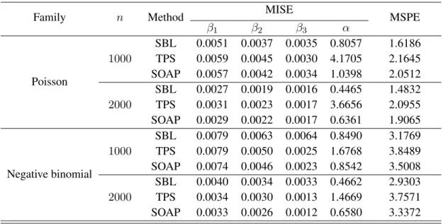
squared prediction error (MSPE). Table 2.1 presents the MISE of β1, β2, β3, α and the 10-fold
cross-validated MSPE, where the SBL results are based on using four interior knots for univariate splines and41
for bivariate splines. Table2.1shows that the performance of our method and the TPS method. All three methods are similar in terms of the estimation ofβk(·)’s, however, our method significantly outperforms
the TPS and SOAP when estimating the bivariate functionα(·), which results in a big improvement of the cross-validated MSPE.
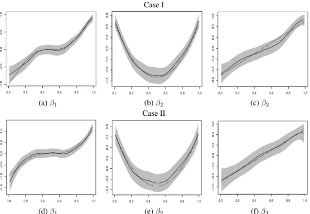
Figure2.4depicts the true univariate functionβk(dotted curve). It also shows the corresponding
esti-matorβbkSBL(solid curve) and the95%SCB forβk(grey bands) from a typical run generated from Case I or
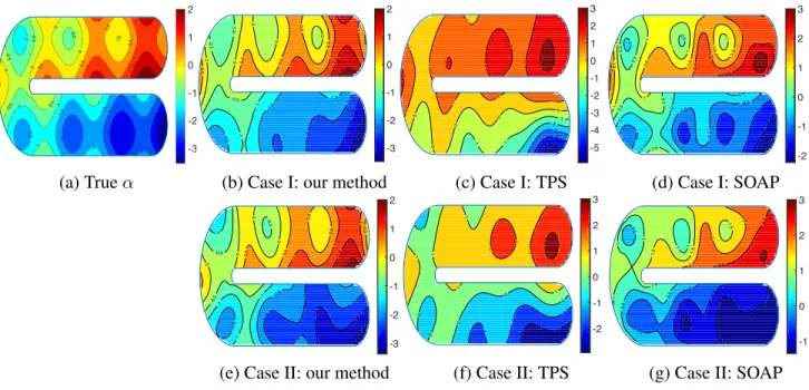
Case II with sample sizen= 2,000, where the estimation and SCB construction are based on four interior quantile knots for the univariate splines and triangulation41 for the bivariate splines. Figure 2.5(b)-(g)
show the contour maps of the estimated bivariate functionsαb over a grid of500×200 points using our
method, TPS and SOAP.
We evaluate the coverage of the proposed SCBs over 20 equally spaced points on[0,1]and test whether the true functions are covered by the SCBs at these points. Table2.2 summarizes the empirical coverage rate of the 95% SCBs from 1000 Monte Carlo experiments. The results clearly show a very good coverage rate of the SCBs.
Figures2.6 and2.7 present the MISEs of the estimators based on different combinations of knots and triangulations for Case I and Case II. For the univariate components, one sees that the MISEs are very similar regardless to the choice of knots and triangulations. For the bivariate functionα, we have found in
Table 2.1 MISE of the functional component estimators and 10-fold cross-validated MSPE.
Family n Method MISE MSPE
β1 β2 β3 α Poisson 1000 SBL 0.0051 0.0037 0.0035 0.8057 1.6186 TPS 0.0059 0.0045 0.0030 4.1705 2.1645 SOAP 0.0057 0.0042 0.0034 1.0398 2.0512 2000 SBL 0.0027 0.0019 0.0016 0.4465 1.4832 TPS 0.0031 0.0023 0.0017 3.6656 2.0955 SOAP 0.0029 0.0022 0.0017 0.6361 1.9065 Negative binomial 1000 SBL 0.0079 0.0063 0.0064 0.8490 3.1769 TPS 0.0079 0.0050 0.0025 1.6768 3.8489 SOAP 0.0074 0.0046 0.0023 0.8542 3.5008 2000 SBL 0.0040 0.0034 0.0033 0.4662 2.9303 TPS 0.0034 0.0030 0.0013 1.4669 3.7571 SOAP 0.0033 0.0026 0.0012 0.6580 3.3372
Table 2.2 The coverage rate of the 95% SCBs for univariate functions.
n Poisson Negative binomial
β1 β2 β3 β1 β2 β3
1000 0.945 0.949 0.967 0.949 0.967 0.960 2000 0.947 0.965 0.979 0.980 0.980 0.970
Case I 0.0 0.2 0.4 0.6 0.8 1.0 − 1.0 − 0.5 0.0 0.5 1.0 x0 0.0 0.2 0.4 0.6 0.8 1.0 − 0.4 − 0.2 0.0 0.2 0.4 0.6 0.8 x0 0.0 0.2 0.4 0.6 0.8 1.0 − 0.6 − 0.4 − 0.2 0.0 0.2 0.4 0.6 x0 (a)β1 (b)β2 (c)β3 Case II 0.0 0.2 0.4 0.6 0.8 1.0 − 1.5 − 1.0 − 0.5 0.0 0.5 1.0 x0 0.0 0.2 0.4 0.6 0.8 1.0 − 0.4 − 0.2 0.0 0.2 0.4 0.6 0.8 x0 0.0 0.2 0.4 0.6 0.8 1.0 − 0.6 − 0.4 − 0.2 0.0 0.2 0.4 0.6 x0 (d)β1 (e)β2 (f)β3
Figure 2.4 Plots ofβk(xk)(dotted curve), the SBL estimator (solid curve) and the 95% SCBs (grey bands),k= 1,2,3, based onn= 2,000observations.
-3 -2.5 -2 -2 -2 -1.5 -1.5 -1.5 -1 -1 -0.5 -0.5 -0.5 0 0 0 0 0 0.5 0.5 0.5 0.5 0.5 1 1 1 1.5 1.5 2 -3 -2 -1 0 1 2 -5 -4 -3 -2 -1 -1 -1 0 0 0 0 0 1 1 1 1 1 1 1 2 2 2 2 2 3 3 -5 -4 -3 -2 -1 0 1 2 3 -2 -1.5 -1 -1 -1 -1 -0.5 -0.5 -0.5 -0.5 0 0 0 0 0 0.5 0.5 0.5 0.5 0.5 0.5 1 1 1 1 1 1 1 1.5 1.5 1.5 1.5 1.5 2 2 2 2 2.5 2.5 3 -2 -1 0 1 2 3
(a) Trueα (b) Case I: our method (c) Case I: TPS (d) Case I: SOAP
-3 -2.5 -2.5 -2 -2 -2 -2 -1.5 -1.5 -1 -1 -1 -1 -0.5 -0.5 -0.5 0 0 0 0 0.5 0.5 0.5 0.5 0.5 1 1 1 1.5 2 -3 -2 -1 0 1 2 -2 -1 -1 -1 0 0 0 0 0 0 1 1 1 1 1 2 2 2 3 -2 -1 0 1 2 3 -1 -1 -1 -0.5 -0.5 0 0 0 0.5 0.5 0.5 1 1 1 1 1 1 1.5 1.5 1.5 2 2 2 2.5 2.5 3 -1 0 1 2 3
(e) Case II: our method (f) Case II: TPS (g) Case II: SOAP
Figure 2.5 Contour maps for the true bivariate function and its estimators.
our simulation studies that there is a minimum adequate value of the number of triangles in the fitting. Fits using fewer than this minimum number of triangles have low statistical accuracy. We have also found that, when this minimum number of triangles is reached, further refining the triangulation will have little effect on the fitting process, but make the computational burden unnecessarily heavy.
Finally, our proposed method is very user-friendly and computationally efficient. Take the case of fitting GGAMs with the Poisson distribution as an example. Remarkably, it takes only 3.1 seconds to estimate all the components in the GGAM with 2,000 observations on a standard PC with processor Core i5 @2.7GHz CPU and 8.00GB RAM. This is extremely fast considering that the entire nonparametric regression is done without WARPing.
2.6.2 Example 2
We conduct another simulation study using the covariates and domain of the crash data analyzed in Section 2.7. We consider the following negative binomial setting: Yi ∼ NB
θ, µi
θ+µi
, whereθ = 2.7,
# T=109 N=2 N=4 N=6 N=8 0.000 0.002 0.004 0.006 0.008 0.010 0.012 # T=163 N=2 N=4 N=6 N=8 # T=237 N=2 N=4 N=6 N=8 # T=109 N=2 N=4 N=6 N=8 0.002 0.004 0.006 0.008 # T=163 N=2 N=4 N=6 N=8 # T=237 N=2 N=4 N=6 N=8 (a)β1 (b)β2 # T=109 N=2 N=4 N=6 N=8 0.000 0.002 0.004 0.006 0.008 0.010 0.012 # T=163 N=2 N=4 N=6 N=8 # T=237 N=2 N=4 N=6 N=8 # T=109 N=2 N=4 N=6 N=8 0.2 0.4 0.6 0.8 # T=163 N=2 N=4 N=6 N=8 # T=237 N=2 N=4 N=6 N=8 (c)β3 (d)α
Figure 2.6 Boxplots of the MISEs of the estimators of functional components in Case I using different combinations of knots and triangulations.
# T=109 N=2 N=4 N=6 N=8 0.000 0.005 0.010 0.015 0.020 # T=163 N=2 N=4 N=6 N=8 # T=237 N=2 N=4 N=6 N=8 # T=109 N=2 N=4 N=6 N=8 0.000 0.005 0.010 0.015 # T=163 N=2 N=4 N=6 N=8 # T=237 N=2 N=4 N=6 N=8 (a)β1 (b)β2 # T=109 N=2 N=4 N=6 N=8 0.000 0.005 0.010 0.015 # T=163 N=2 N=4 N=6 N=8 # T=237 N=2 N=4 N=6 N=8 # T=109 N=2 N=4 N=6 N=8 0.2 0.4 0.6 0.8 1.0 1.2 1.4 # T=163 N=2 N=4 N=6 N=8 # T=237 N=2 N=4 N=6 N=8 (c)β3 (d)α
Figure 2.7 Boxplots of the MISEs of the estimators of functional components in Case II using different combinations of knots and triangulations.
Table 2.3 The MISE of the estimators of the component functions and the coverage rate of the 95% SCB for the univariate functions.
Measurement Component β1 β2 β3 β4 β5 β6 MISE 0.0025 0.0017 0.0015 0.0019 0.0033 0.0017 Coverage 0.786 0.959 0.958 0.954 0.890 0.964 β7 β8 β9 β10 β11 β12 α MISE 0.0021 0.0018 0.0016 0.0028 0.0030 0.0032 0.0318 Coverage 0.962 0.963 0.967 0.973 0.965 0.991 –
the crash dataset described in Section2.7. The significant univariate functions and bivariate function are set to be the same as the estimates obtained in the crash data analysis, and insignificant univariate functions are set as zero.
The average MISE of each functional component from 1000 Monte Carlo experiments is reported in Table2.3. From Table2.3, one sees that the MISE are all very small which indicates our method performs very well. We also examine the behavior of the proposed SCBs for the univariate functions. The “coverage” rows in Table2.3summarize the empirical coverage rate of the 95% SCBs from 1000 Monte Carlo experi-ments, and the results seem to be very reasonable. See Figures2.8and2.9for the estimators and the SCBs from a typical simulation trial.
2.7 Application to Crash Data 2.7.1 Domain of Interest
Traffic crashes have been one of the major sources of fatalities and injuries in the United States. Crash frequency analysis is critical for developing and implementing effective safety improvement programs. In this study, we are interested in identifying the spatial pattern of crashes and investigating how demographic, economic, and commuting factors influence crash frequency after the spatial effect is adjusted.
This study focuses on the Tampa-St. Petersburg urbanized area, including Tampa, Clearwater, and St. Petersburg, is a major populated area surrounding Tampa Bay on the west coast of Florida, United States. The area consists of 1,761 census block groups, as shown in Figure2.1(a) and2.1(b). A census block group
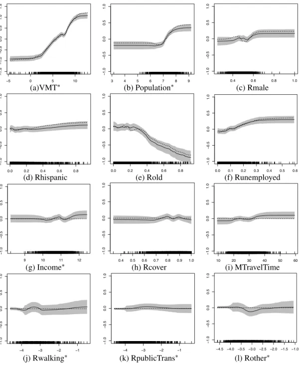
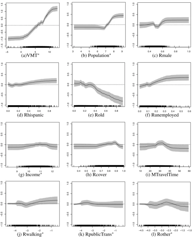
−5 0 5 10 − 1.5 − 1.0 − 0.5 0.0 0.5 1.0 1.5 x0 3 4 5 6 7 8 9 − 1.0 − 0.5 0.0 0.5 1.0 x0 0.4 0.6 0.8 1.0 − 1.0 − 0.5 0.0 0.5 1.0 x0
(a)VMT∗ (b) Population∗ (c) Rmale
0.0 0.2 0.4 0.6 0.8 − 1.0 − 0.5 0.0 0.5 1.0 x0 0.0 0.2 0.4 0.6 0.8 − 1.0 − 0.5 0.0 0.5 1.0 x0 0.0 0.1 0.2 0.3 0.4 0.5 0.6 − 1.0 − 0.5 0.0 0.5 1.0 x0
(d) Rhispanic (e) Rold (f) Runemployed
9 10 11 12 − 1.0 − 0.5 0.0 0.5 1.0 x0 0.4 0.5 0.6 0.7 0.8 0.9 1.0 − 1.0 − 0.5 0.0 0.5 1.0 x0 10 20 30 40 50 60 − 1.0 − 0.5 0.0 0.5 1.0 x0
(g) Income∗ (h) Rcover (i) MTravelTime
−4 −3 −2 −1 − 1.0 − 0.5 0.0 0.5 1.0 x0 −4 −3 −2 −1 − 1.0 − 0.5 0.0 0.5 1.0 x0 −4.5 −4.0 −3.5 −3.0 −2.5 −2.0 −1.5 −1.0 − 1.0 − 0.5 0.0 0.5 1.0 x0
(j) Rwalking∗ (k) RpublicTrans∗ (l) Rother∗
Figure 2.8 Plots of the true function (dashed line), its SBL estimator (black curve) and the 95% SCB (grey band).