A Framework to improve Turbulence Models using Full-field Inversion and Machine Learning

(1)

A Framework to improve Turbulence Models using

Full-field Inversion and Machine Learning

by

Anand Pratap Singh

A dissertation submitted in partial fulfillment of the requirements for the degree of

Doctor of Philosophy (Aerospace Engineering) in The University of Michigan

2018

Doctoral Committee:

Associate Professor Karthik Duraisamy, Chair Associate Professor Krzysztof J. Fidkowski Professor Krishnakumar R. Garikipati

(2)

“The truth is,

most of us

discover where

we are heading

when we arrive.”

Bill Watterson Calvin and Hobbes

(3)

Anand Pratap Singh [email protected] ORCID iD: 0000-0002-1954-6375

c

(4)

To my mother for her courage and sacrifices and to my late father for his dreams.

(5)

ACKNOWLEDGEMENTS

I have to confess, joining the PhD program, I was not sure about what I was going to do or what I was really interested in. The only thing I was sure of was that I loved being a student. However, thanks to my advisor Prof. Karthik Duraisamy and others, my graduate work has been extremely fruitful. In all honesty, the marathon of a PhD is never entirely fun, there were both good days and bad days, but it all was completely worth it. As John Donne said, no man is an island. This work could not be possible without an amalgamation of support from a number of people. I know I cannot possibly list everyone in this section.

I could not have asked for a better advisor than Prof. Duraisamy. He is tolerant towards what I will call productive procrastination, where I could work on a projects and ideas I loved but were not directly related to my PhD thesis. He was, in hindsight, kind enough to push me at times, and brutally honest. He was extremely patient and helpful with my writing. His mentoring style had me be more scientifically independent. Above everything, I am grateful for his patience during the toughest time of my personal life.

I would like to thank the committee members, Prof. Garikipati, Prof. Fidkowski, and Prof. Powell for their guidance and helpful suggestions during the course of this work and the preparation of this document.

(6)

with the TURNS code when I was just starting my PhD and during my internship at Altair towards the end, which really boosted my graduate work. I thank Helen for her generous help with all the coursework during the first year - most of which I was careless enough to miss, and also for her help throughout the projects. I dont know if I should thank Eric, Nick and Ayoub for all our crazy shenanigans. In all seriousness, they have been great friends. I especially thank Yaser, Eric, Nick, and Walt for meticulously proofreading this document. All of the group members have each contributed in their own way to this work and also towards my personal development. Special mention and thanks to all of my FXB friends, Yuki, Chris, Devina for all the happy, fun times and memories. Brad, Wai Lee, and Yuntao were my first office-mates who really helped me settle were always approachable and warm. They played an important role as I progressed through my graduate work.

I would have never been able to do this without the unwavering support of my family. I thank my wife Arushi, who has been a pillar of support during the entire duration. I thank my parents Kanti and Dr. Ramesh Kumar Deshwali - their inspi-ration and sacrifices has brought me to where I am today. I am the luckiest person to be able to look up to them. I thank my sister Dr. Akanksha Deshwali for always believing in me.

This acknowledgement section took the longest to write, I really didn’t want to write it at all. In a symbolic way this section probably marks the end of my student life, however, I will always continue to learn.

Funding for this work was provided by the NASA Aeronautics Research Institute under the Leading Edge Aeronautics Research for NASA program (technical monitors: Koushik Datta and Gary Coleman) and DARPA under the EQUiPS project (technical monitor: Dr. Fariba Fahroo). Computing resources were provided by the NSF via

(7)

grant MRI: Acquisition of Conflux, A Novel Platform for Data-Driven Computational Physics (technical monitor: Ed Walker).

(8)

LIST OF TABLES

Table

4.1 List of ML models along with the data and flow-features used for training. . . 77 6.1 List of airfoil shapes and flow-conditions for which inverse problems

are solved. . . 110 6.2 List of ML models and the inverse solutions used for training. The

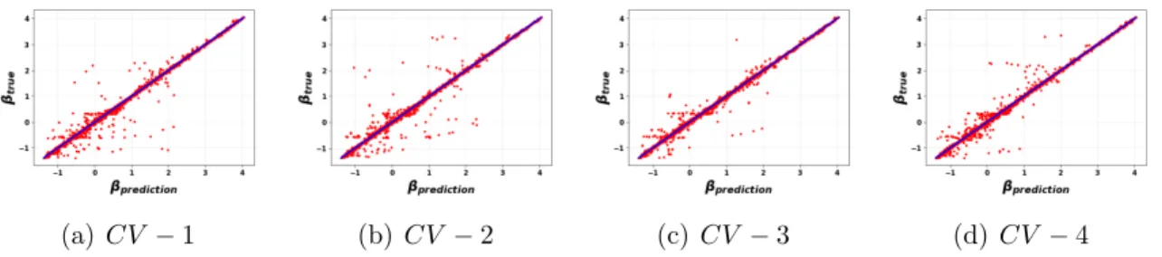
main predictive model is labeled P. . . 117 6.3 Results of 5-fold cross-validation. The error metric is the coefficient

(12)

LIST OF FIGURES

Figure

1.1 A notional time-line of development in turbulence simulations. . . . 4 2.1 Schematic of the field-inversion and machine-learning (FIML)

show-ing the offline components which includes inference and trainshow-ing of the machine learning model and the online prediction. . . 24 2.2 Flowchart depicting the connection between the forward and the

in-verse problem. . . 27 2.3 Bayesian inference involves calculation of posterior probability

distri-bution using prior distridistri-bution and the likelihood. . . 29 2.4 L-curves are used to fix the value of λ, but it requires solution to

many inverse problems for different values of λ’s. . . 33 2.5 Solving an inverse problem is equivalent to solving an optimization

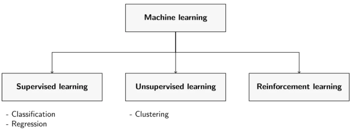
problem with an appropriate objective function, J, and the discrep-ancyδ being the design variable. . . 34 2.6 Machine learning problem can be classified as either supervised

learn-ing, unsupervised learnlearn-ing, or reinforcement learning. . . 38 2.7 Schematic describing the process of cross-validation (CV). The

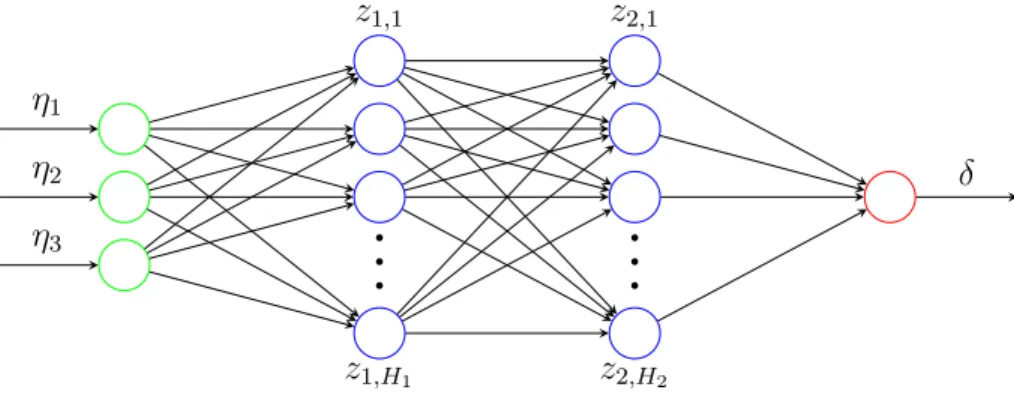
ex-ample uses a 3-fold CV. The figure is adapted from https://tex. stackexchange.com/a/154121. . . 39 2.8 Network diagram for a feed-forward NN with three inputs, two hidden

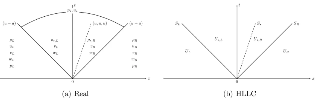
layers, and one output. . . 44 3.1 Characteristics of the actual Euler equations and the HLLC

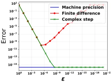
approx-imation. . . 54 3.2 Error in the derivative calculation for a test function functionf(x) =

x4 _at_x_{= 1. . . .} ₆₀

4.1 Flow setup and geometry for the concave curvature case. The inlet boundary layer is generated using a zero pressure gradient flat plate simulation. . . 66 4.2 Comparison of the skin friction and the surface pressure coefficients at

the lower wall using the LES, SA model, and SA–RC model. The skin friction predictions are much improved using SA–RC. S represents the streamwise distance. . . 67

(13)

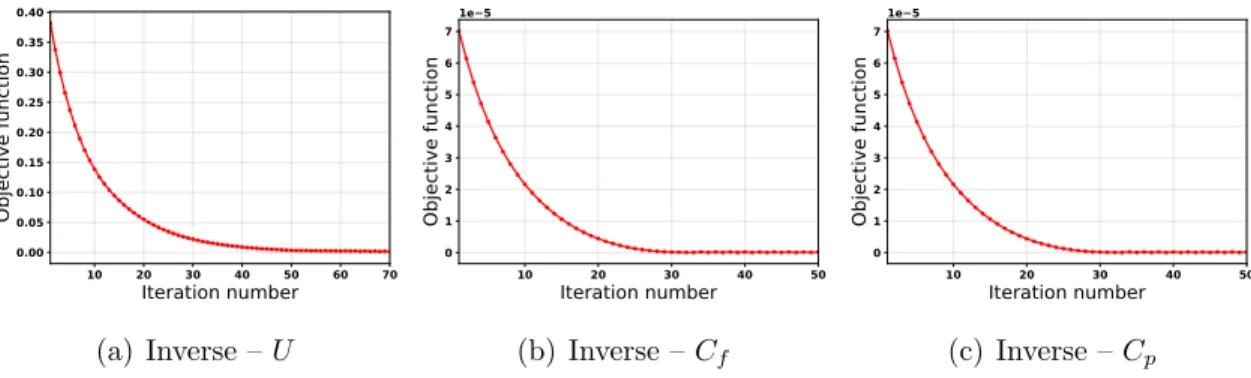
4.3 Convergence of the steepest descent algorithm for the three inverse problems. . . 67 4.4 Inferred non-dimensional discrepancy field (β(x)) using three

differ-ent objective functions and the equivaldiffer-ent term fr1 in the SA–RC

model. . . 68 4.5 Inferred dimensional discrepancy field (δ(x)) using three different

ob-jective functions and the equivalent term in the SA–RC model. . . . 69 4.6 Comparison of the skin friction and surface pressure coefficients at

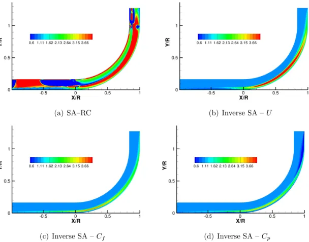
the lower wall using the SA–RC, baseline SA model, and inverse SA model using three different objective functions. S represents the streamwise distance. . . 69 4.7 Tangential velocity profile at different streamwise locations. θ = 0◦

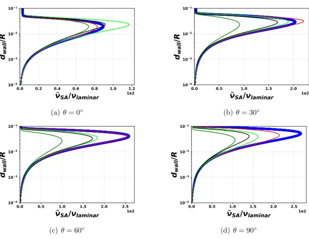
marks the onset of the curvature andθ = 90◦ marks its end. . . 70 4.8 SA eddy-viscosity profile at different streamwise locations. θ = 0◦

marks the onset of the curvature andθ = 90◦ _{marks its end. . . . .} ₇₁

4.9 Reynolds shear-stress−u0

ru0θ profile at different streamwise locations.

θ = 0◦ _{marks the onset of the curvature and}_θ _{= 90}◦ _{marks its end.} ₇₂

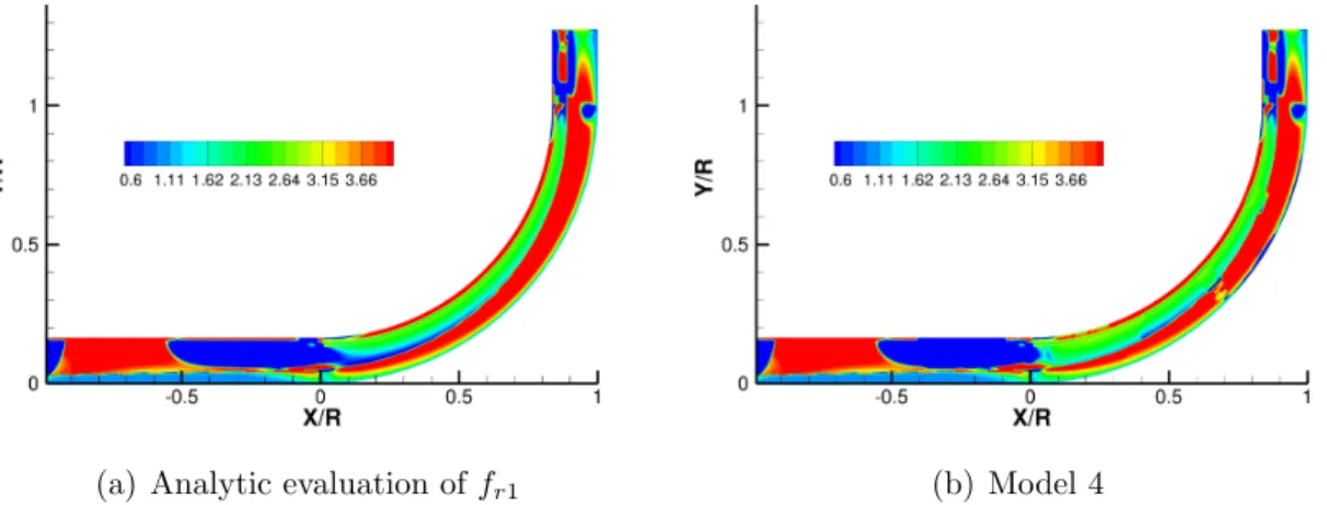
4.10 Scatter plot of the two features used in SA–RC model. The features are evaluated at the inverse solution and are colored by: (a) Produc-tion, (b) analytic fr1, and (c) inferred β. The region of interest is

enclosed in the green rectangle. Outside this region the production term is zero. Therefore, differences between fr1 and β outside this

region will have minimal impact on the flow solution. . . 76 4.11 Test results for Model 2 using 4-fold cross-validation and the

Ad-aBoost algorithm. . . 78 4.12 Comparison of the skin friction and the surface pressure coefficients

at the lower wall using the SA–RC, the baseline SA model, and the ML augmented SA model 2. S represents the streamwise distance. . 79 4.13 Reynolds shear-stress profile at different streamwise locations. θ = 0◦

marks the onset of the curvature and θ = 90◦ _{marks the end of the}

curvature. Legends: —SA–RC,—Base SA,—Inverse SA -Cf and

— ML SA model 2. . . 79 4.14 Inferred discrepancy field β(x) using Cf and the ML SA model 2

predicted β(η) at the converged solution. . . 80 4.15 Test results for Model 22 using 4-fold CV and the AdaBoost algorithm. 80 4.16 Comparison of the skin friction and the surface pressure coefficients

at the lower wall using the SA–RC, baseline SA model, and ML augmented SA model 22. S represents the streamwise distance. . . . 81 4.17 Reynolds shear-stress profile at different streamwise locations. θ = 0◦

curvature. Legends: — SA–RC,— Base SA,— Inverse SA - U and

— ML SA model 22. . . 81 4.18 Inferred discrepancy field β(x) using U and the ML SA model 22

(14)

4.19 Comparison of the skin friction and the surface pressure coefficients at the lower wall using the SA–RC, baseline SA model, and ensembles of various ML augmented SA model. S represents the streamwise distance. . . 83 4.20 Reynolds shear-stress profile at different streamwise locations. θ = 0◦

curvature. Legends: — SA–RC,— Base SA, and —ML SA model 4. 83 4.21 Comparison of the analytic correctionfr1 with the ML reconstruction

of fr1. . . 84

4.22 Absolute difference between the analytic correction fr1 and the ML

reconstruction of fr1. . . 84

5.1 Labels for the various flow cases based on variation in the bump height and inlet momentum thickness. Inverse solutions for the cases marked in the red box are used to train model P. . . 88 5.2 Comparison of the skin friction and pressure for bumps with different

bump heights from LES. . . 89 5.3 Comparison of the skin friction and pressure for 3 different inlet

mo-mentum thicknesses from LES. . . 89 5.4 Comparison of X-velocity at different streamwise locations. . . 90 5.5 Comparison of turbulent shear-stress at different streamwise locations. 90 5.6 Contour plots of mean X-velocity and TKE for H20-1. . . 91 5.7 Contour plots of mean X-velocity and TKE for H42-1. . . 91 5.8 The misfit (J1) and the regularization (J2) terms are used to fix the

regularization constant. For this representative case λelbow≈10−6. . 93 5.9 Skin friction for all the 11 cases. Shaded red region contains inverse

solutions for various 10−10 _{< λ <} ₁₀−6_{. Legend:} _— _LES, _— _base k−ω and — inverse k−ω using Cf. . . 94 5.10 Inferred spatial discrepancy field β(x) using skin friction data. The

thick black line marks the boundary layer edge. . . 95 5.11 Comparison of skin friction obtained after inference using data for

the skin friction and the full-field velocity. . . 95 5.12 Flow solution at X/C = ₋0.16 obtained after inference using data

for the skin friction and the full field velocity. . . 96 5.13 Flow solution atX/C = 0 obtained after inference using data for the

skin friction and the full field velocity. . . 96 5.14 Flow solution at X/C = 0.33 obtained after inference using data for

the skin friction and the full field velocity. . . 97 5.15 Flow solution at X/C = 0.66 obtained after inference using data for

the skin friction and the full field velocity. . . 98 5.18 Test results for modelP using 2-fold CV and the AdaBoost algorithm. 99

(15)

5.19 Skin friction predictions using the baselinek₋ω (solid line) and the AdaBoost-augmented model P (dashed line). . . 99 5.20 Skin friction prediction for all the 11 cases. Thin magenta lines

repre-sent predictions using an ensemble of machine-learned models trained on different combinations of the inverse solutions. Legend: — LES,

— base k−ω and — AdaBoost augmented k−ω using model P. . 100 5.21 Flow solution at X/C = ₋0.16 using AdaBoost augmented model

P. Thin magenta lines represent predictions using an ensemble of machine-learned models trained on different combinations of the in-verse solutions. . . 100 5.22 Flow solution atX/C = 0 using AdaBoost augmented modelP. Thin

magenta lines represent predictions using an ensemble of machine-learned models trained on different combinations of the inverse solu-tions. . . 101 5.23 Flow solution at X/C = 0.33 using AdaBoost augmented model

P. Thin magenta lines represent predictions using an ensemble of machine-learned models trained on different combinations of the in-verse solutions. . . 101 5.24 Flow solution at X/C = 0.66 using AdaBoost augmented model

P. Thin magenta lines represent predictions using an ensemble of machine-learned models trained on different combinations of the in-verse solutions. . . 102 5.27 Pairwise scatter plots of the flow features used for training. Features

for all the cases are shown in red and the features used to train model

P are shown in green. . . 102 6.1 Lift vs. angle of attack plot for the S809 airfoil at a Reynolds number

of 2 Million. . . 105 6.2 Three different airfoil shapes are used for training and testing the

ML-based augmentation. . . 106 6.3 Samples of figures used to extract data for this work. These figures

are reproduced from [96]. . . 106 6.4 A body fitted C-mesh is used with 291 points in the wrap around

direction and 111 points in the perpendicular direction. . . 107 6.5 Surface pressure using the baseline SA model (green) and experiment

(blue) for the S809 airfoil atRe= 2 Million. . . 108 6.6 Velocity fields using the baseline SA model for the S809 airfoil at

(16)

6.7 Surface pressure for the S809 airfoil at Re= 2 Million andα= 14◦_. ₁₁₀

6.8 Inferred discrepancy using different data types for the S809 airfoil at α = 19◦ _{and Re = 2 Million. The discrepancy deviates from the}

baseline value of unity only inside the region marked with the black curve. . . 111 6.9 Inferred discrepancy fields for the S809 airfoil at Re = 2 Million. The

discrepancy deviates from the baseline value of unity only inside the region marked with the black curve. . . 112 6.10 Surface pressure obtained using inferred discrepancy fields for the

S809 airfoil at Re = 2 Million. . . 113 6.11 Streamline and contour plots of the X-velocity for the S809 airfoil at

Re= 2 Million andα= 14◦_{. . . 114}

6.12 Eddy-viscosity for the S809 airfoil at Re= 2 Million andα = 14◦. . 115 6.13 Lift and drag coefficients obtained using inferred discrepancy fields

for the S809 airfoil at Re = 2 Million. . . 116 6.14 Neural network training for modelP. x and y axes correspond to the

true and predicted values, respectively. . . 118 6.15 Comparison of inverse and NN-augmented predictions (using model

P) for S809 airfoil at α= 14◦ and Re= 2×106. . . 118 6.16 Streamlines and X-velocity contours for the S809 airfoil at Re =

2×106 _and _α _{= 14}◦_{. . . 119}

6.17 NN-augmented SA prediction for the S814 airfoil using model P. Legend: —Experiment,—base SA and—neural network SA model

P. . . 120 6.18 NN-augmented SA prediction for the S805 airfoil using model P.

Legend: —Experiment,—base SA and—neural network SA model

P. . . 120 6.19 NN-augmented SA prediction for the S809 airfoil using model P.

Legend: —Experiment,—base SA and—neural network SA model

P. . . 121 6.20 Surface pressure for the S809 airfoil at Re = 2 × 106 _and _α ₌

{16◦_,₁₈◦_,₂₀◦

}. Refer Fig. 6.15(c) for legend. Not to scale. . . 121 6.21 Surface pressure for the S805 airfoil at Re = 1 × 106 _and _α ₌

{12◦_,₁₄◦_}_{. Refer Fig. 6.15(c) for legend. Experimental pressure}

is shown only for the upper surface. Not to scale. . . 122 6.22 Surface pressure for the S814 airfoil at Re = 1.5 ×106 _and _α ₌

{16◦_,₁₈◦_,₂₀◦_}_{. Refer Fig. 6.15(c) for legend. Experimental pressure}

is shown only for the upper surface. Inversion is not performed for this case. Not to scale. . . 122 6.23 Pressure and skin friction (using model P) for the S809 airfoil at

Re = 2_× 106 _and _α _{= 14}◦ _{using grids of different spatial}

resolu-tions. Solutions of both the base SA model and the neural network augmented SA are grid converged. . . 123 6.24 Predicted surface pressure for the S809 airfoil at Re= 2_×106 _using

(17)

6.25 NN-augmented SA prediction using AcuSolve for the S809 airfoil us-ing model P. Legend: — Experiment, — base SA and — neural network SA model P. . . 124 6.26 AcuSolve’s convergence history for S809 airfoil at Re = 2 _× 106_,

(18)

LIST OF ABBREVIATIONS

APG adverse pressure gradient

CV cross-validation

DES detached-eddy simulation

DNS direct numerical simulation

FANN fast artificial neural network

FIML field-inversion and machine-learning

LES large-eddy simulation

MAP maximum a-posteriori

MCMC Markov-chain Monte Carlo

ML machine-learning

NN neural-network

NS Navier-Stokes

RANS Reynolds-averaged Navier-Stokes

SA Spalart-Allmaras

TKE turbulence kinetic energy

(19)

ABSTRACT

Accurate prediction of turbulent flows remains a barrier to the widespread use of computational fluid dynamics in analysis and design. Since practical wall-bounded turbulent flows involve a very wide range of length and time scales, it is intractable to resolve all relevant scales, due to limitations in computational power. The usual tools for predictions, in order of their accuracy, includes direct numerical simulation (DNS), large-eddy simulation (LES), and Reynolds-averaged Navier-Stokes (RANS) based models.

DNS and LES will continue to be prohibitively expensive for analysis of high Reynolds number wall-bounded flows for at least two more decades and for much longer for design applications. At the same time, the high-quality data generated by such simulations provides detailed information about turbulence physics in affordable problems. Experimental measurements have the potential to offer limited data in more practical regimes. However, data from simulations and experiments are mostly used for validation, but not directly in model improvement.

This thesis presents a generalized framework of data-augmented modeling, which we refer to as field-inversion and machine-learning (FIML). FIML is utilized to develop augmentations to RANS-based models using data from DNS, LES or experiments. This framework involves the solution of multiple inverse problems to infer spatial dis-crepancies in a baseline turbulence model by minimizing the misfit between data and predictions. Solving the inverse problem to infer the spatial discrepancy field allows

(20)

the use of a wide variety and fidelity of data. Inferring the field discrepancy using this approach connects the data and the turbulence model in a manner consistent with the underlying assumptions in the baseline model. Several such discrepancy fields are used as inputs to a machine learning procedure, which in turn reconstructs corrective functional forms in terms of local flow quantities. The machine-learned discrepancy is then embedded within existing turbulence closures, resulting in a partial differential equation/machine learning hybrid, and utilized for prediction.

The field-inversion and machine-learning (FIML) framework is applied to augment the Spalart-Allmaras (SA) and the Wilcox’s k ₋ ω model and for flows involving curvature, adverse pressure gradients, and separation. The value of the framework is demonstrated by augmenting the SA model for massively separated flows over airfoil using lift data for just one airfoil. The augmented SA model is able to accurately predict the surface pressure, the point of separation and the maximum lift – even for Reynolds numbers and airfoil shapes not used for training the model. The portability of the augmented model is demonstrated by utilizing in-house finite-volume flow solver with FIML to develop augmentations and embedding them in a commercial finite-element solver. The implication is that the machine-learning (ML)-augmented model can thus be used in a fashion that is similar to present-day turbulence model.

While the results presented in this thesis are limited to turbulence modeling, the FIML framework represents a general physics-constrained data-driven paradigm that can be applied to augment models governed by partial differential equations.

(21)

CHAPTER I

Introduction

Driven by an exponential growth in computational power, reliance on simulations has grown in every scientific field and the trend is expected to continue. Computa-tional models are increasingly being used to drive design and development of engi-neering products. The rise in high fidelity simulations has led to better understanding of physical processes, which is being used to fill gaps in existing knowledge and to improve lower order theories/models.

Simulations of physical systems involve the solution of mathematical equations in their discretized forms. The accuracy of the solution depends on the correctness of the underlying mathematical model and the accuracy of the discretization approach. In other words, to obtain accurate results, the right set of equations should be solved using the right techniques.

Physical modeling involves the development of a mathematical relationship to describe a system. Such relationships may be derived based on first principles. For example, the governing equations of fluid dynamics, the Navier-Stokes (NS) equations, are the embodiments of the conservation of mass, momentum, and energy. In some cases, the models are purely empirical and are estimated by fitting the model to the data. Most practical models lie between the two extremes, with a blend of first principles and a few empirical relationships. All the examples discussed in the present

(22)

work belong to this last category.

The quality of the solution of a discretized model often requires a trade-off between computational power and accuracy – particularly in the simulation of turbulent flows, where the difference between the smallest and the largest flow structures can be many orders of magnitude. Currently available computational power is not sufficient to resolve all the scales in such flows, and a fully-resolved simulation will not be attainable for the next few decades. Even when viable, it will require months of runtime on the world’s most powerful computers, which will restrict its utility in an iterative design process.

Accurate prediction of turbulence is important as an increase in turbulence leads to enhanced mixing, heat transfer, and momentum transfer. These are quantities of interest in many situations and can affect critical design decisions. The inability of accurately simulating turbulent fluid flow in an affordable manner has led to lower-fidelity models, where the unresolved physics (small-scale) is modeled in terms of the resolved quantities (large scale). Examples of such models include large-eddy simulation (LES) and Reynolds-averaged Navier-Stokes (RANS) based models.

This chapter highlights properties of turbulent flows which lead to modeling diffi-culties. Various levels and methods of turbulence modeling are discussed along with some of their strengths and weaknesses. A case is made for data-driven augmentation of turbulence models. We discuss previous and ongoing efforts of using data-driven techniques to improve the prediction of turbulence. Against this backdrop, the mo-tivation and the contribution of this work are presented. This discussion is tailored to provide context to the current work and is by no means exhaustive. Readers are referred to [74] for a more detailed discussion of turbulence modeling.

(23)

1.1 Fluid Flow and Turbulence

Turbulent flows are characterized by seemingly random structures or eddies. A non-dimensionless quantity, Reynolds numberRe, describes the capability of the flow to transition from a laminar to a turbulent state. The Reynolds number, Re, is defined as the ratio of the momentum of the flow to the viscous force and is given by

Re= U L

ν , (1.1)

where U and L are characteristic velocity and length scales and ν is the kinematic viscosity of the fluid.

In a high Reynolds number flow, the size of the smallest and the largest eddies can differ by many orders of magnitude. Most flows of practical interest in the aerospace community are high Reynolds number flows, which are inherently turbulent or transition to turbulence from a laminar state. The typical Reynolds number of the flow over the wing of a commercial jet, based on the wing chord, is O(108_).

The smallest scales in a turbulent flow were first estimated by A.N. Kolmogorov in 1941[50]. According to the Kolmogorov hypothesis, at sufficiently high Reynolds numbers, small-scale turbulent motions are statistically isotropic and the statistics of the small-scale motion is uniquely determined by the laminar kinematic viscosity ν

and specific dissipation. The associated scales, also know as Kolmogorov microscales can then be defined by dimensional analysis

η≡ ν3 1/4 , uη ≡(ν)1/4, τη ≡ ν 1/2 , (1.2)

where,η,uη and τη are the length, velocity and time scale, respectively. Further, the small scales dissipate the energy, and therefore the relationship between the larger scales and smaller scales can be estimated as =U3_/L_{, where U and L are the large}

(24)

1880 1900 1920 1940 1960 1980 2000

Eddy Viscosity concept Prandtl Mixing Length k First DNS, Channel Flow W

ilc ox k Me nt er k , S -A DES 103 107 1011 1015 1019 1023 FLOPS Full airplane DNS

Figure 1.1: A notional time-line of development in turbulence simulations. scale velocity and length scales. This results in the following relationships,

η/L_∼Re−3/4, uη/U ∼Re−1/4, τη/T ∼Re−1/2. (1.3)

The smallest length and time scales therefore depend on the Reynolds number of the flow. These range of scales makes it hard to solve the NS equations numerically with sufficient resolution for high Reynolds number flows.

1.2 Turbulence Modeling

The Navier-Stokes (NS) equations are non-linear partial differential equations and the non-linearity leads to a complex interaction between different scales of the flow. We solve the NS equations computationally, by discretizing them in some form. For this work, we focus on a mesh-based discretization.

The mesh resolution–the distance between two neighboring mesh points–governs the quality of the solution along with the numerical scheme. If all the scales in a flow are resolved, both in space and time, the solution is fully resolved and can be considered on par with the analytical solution1_{. However, most high Reynolds}

number simulations are not fully resolved because of excessive requirements of the 1_{Numerical errors associated with finite precision of the computers are always present.}

(25)

computational resources. Such under-resolved simulations requires modeling of the unresolved scales, as they interact and affect the resolved scales via transfer of en-ergy and momentum. An under-resolved simulation without such modeling would be inaccurate.

Models of turbulence range from fully-resolved to resolving only the ensemble average of the inherently unsteady turbulent flow. All the models of turbulent flows are however based on the NS equations. Various levels of models are discussed in the following sections.

1.2.1 Direct Numerical Simulation

In a direct numerical simulation (DNS), the NS equations are solved numerically, on a computational mesh, which is fine enough to resolve all the turbulent scales. Using the Einstein notation, the unsteady incompressible NS equations are given by,

∂ui ∂xi = 0 (1.4) ∂ui ∂t + ∂uiuj ∂xj =−1 ρ ∂p ∂xi +ν ∂ 2_u i ∂xj∂xj i= 1,2,3 (1.5) where, uis the velocity vector, pand ρare the pressure, and density, respectively.

In three dimensions, in order to resolve the smallest length scale, η, the number of grid points grows as (Re3/4₎3 _≡_Re9/4 _{(using equations 1.3). The number of time}

steps to resolve the time scale,τη, grows asRe1/2. Therefore the effective work units increase as _≈ Re3_{. A doubling in Reynolds number requires eight times increase in}

the work units which translates to a proportional increase in computational time and resources. This simple estimation does not include the complexity of the algorithm used to numerically solve the NS equations, which adds to the overall complexity.

(26)

num-however, provide a very detailed description of the flow and are used to understand turbulence phenomena for simple canonical flows at low Reynolds numbers. Hence, DNS for simpler flows in channels, or pipes have been performed, and the knowledge has been extrapolated to improve lower order models[66, 53, 52, 30].

Fig. 1.2 shows an estimate of various milestones in the field of turbulence compu-tations along with the increase in the processing power of the computers, calculated as floating-point operations per second (FLOPS). Also, marked is the processing power required for a full airplane simulation. It is expected that the milestone will not be reached for at least next few decades. Therefore, models which do not resolve all the scales will maintain their importance in engineering predictions.

Even if fully-resolved simulations are achievable, a design process which requires multiple solutions for perturbed geometry or flow conditions will maintain the need for less expensive models. In such situations, data from fully-resolved simulations could be used to augment the lower order models, and both levels of models can co-exist in symbiosis.

1.2.2 Large Eddy Simulation

In a large-eddy simulation (LES), the larger turbulent scales are resolved while the effects of the small scales are modeled. A filtering operation is defined and applied to the NS equations, which results in the following filtered continuity and momentum equations ∂u¯i ∂xi = 0, (1.6) ∂u¯i ∂t + ¯uj ∂u¯i ∂xj =₋1 ρ ∂p¯ ∂xi +ν ∂ 2_u_¯ i ∂xj∂xj − ∂τij ∂xj , (1.7)

where ¯φ represents the filtered (or resolved) φ, and τij =uiuj−u¯iu¯j. The filtering is typically implicitly performed by the mesh, as the resolution of the mesh governs the lowest length scale that can be resolved.

(27)

The filtered momentum equation contains a tensorial term τij, referred to as the Smagorinsky (SGS) stress tensor, which is a function of the unresolved scales uiuj. This leads to a closure problem. The tensorτij is therefore modeled to close the equa-tions. A simple model, referred to as the Smagorinsky, calculates effective viscosity

νt such that, τij =−2νtS¯ij, (1.8) where ¯Sij = 1₂ ∂u¯i ∂xj + ∂u¯j ∂xi

. The eddy-viscosity is assumed to be the function of mesh resolution and is given by the following relation,

νt = (Cs∆g)2 q

2 ¯SijS¯ij, (1.9)

where Cs is a model constant and ∆g is a measure of mesh spacing. The model is a function of the mesh spacing as the filtering operation depends on the mesh resolution. The filtered equations, along with the closure model are then solved numerically.

In the near-wall region, the number of required mesh points increases as_≈Re1.8_[16],

which renders LES for high Reynolds number flows involving walls computationally intractable. Wall models have been proposed to model the near wall region to relax the resolution requirements. A robust and accurate modeling of wall effects remains a research problem. Performing a well-resolved and accurate LES requires signifi-cant computational resources and expertise, which has prevented it from becoming an industry workhorse.

1.2.3 Reynolds-averaged Navier-Stokes

RANS-based models are the most popular and widely used turbulence models. RANS-based models are relatively inexpensive, numerically robust, and require a low

(28)

development has led to sufficiently accurate models in many flow problems.

In a RANS setting, the flow variables are decomposed as the sum of two compo-nents: ensemble average, and fluctuation. The former part is resolved both in space and time and the effects of the later part is modeled. The decomposition has the following property,

φ = ¯φ+φ0 (1.10)

¯

φ0

= 0 (1.11)

where, ¯φ is the ensemble average of φ and φ0 is the fluctuation. The ensemble av-eraging operation, when applied to the NS equations, results in the following RANS equations ∂u¯i ∂xi = 0, (1.12) ∂u¯i ∂t + ¯uj ∂u¯i ∂xj =₋1 ρ ∂p¯ ∂xi +ν ∂ 2_u_¯ i ∂xj∂xj − ∂u0 iu0j ∂xj . (1.13)

Similar to LES, the averaging leads to a closure problem because of the term u0

iu0j. This term requires knowledge of the fluctuations in velocity–which are not resolved– and therefore needs to be modeled in terms of the averaged quantities.

The unclosed termu0

iu0j referred to as the Reynolds stress tensor, has some charac-teristics analogous to the viscous stress. The addition of this term leads to an effective increase in the diffusivity in the flow. Consequently, the term has been modeled based on analogies to kinetic theory, which leads to a model similar to molecular diffusion. It is also possible to derive transport equations for the Reynolds stresses starting with the NS equations. However, such equations are also unclosed as they require further higher order correlations (sec 1.4).

The various models for the Reynolds stresses are discussed in the following sec-tions.

(29)

1.3 Eddy Viscosity-based Models

The simplest models for the Reynolds stresses are derived based on analogies between the Reynolds stress and the viscous stress. An effective additional viscosity, eddy-viscosity or turbulent viscosity, is defined. The Reynolds stresses are then given by a relation identical to the viscous diffusivity,

−u0

iu0j = 2νtSij, (1.14)

where Sij is the mean strain rate tensor and νt is the eddy-viscosity. Consequently, the problem is transformed into that of estimating the eddy-viscosity instead of six Reynolds stress components.

While the analogy between the molecular viscosity and the eddy-viscosity reduces the complexity in modeling, it is built on assumptions which are not strictly valid in a turbulent flow. The molecular timescale is much smaller than the flow timescale, while the turbulence timescale and the flow timescale can be comparable. Therefore, the implicit assumption of stress being proportional to strain or equilibrium is almost never valid.

The eddy-viscosity assumption also assumes that the turbulent Reynolds stresses are isotropic, which is rarely valid (for instance, in the near-wall region). In wall-bounded flows, the blocking effects of the wall inhibits the wall-normal component of the Reynolds stresses more than the other components.

Despite overarching simplifications and its shortcomings, eddy-viscosity based models provide sufficiently accurate results for simple attached flows. Because of their simplicity, eddy-viscosity-based models form the workhorse of the industrial design and analysis.

In the subsequent sections, we discuss different types of eddy-viscosity models. The models range from simple algebraic relationships to those containing multiple

(30)

transport equations with highly non-linear source terms. Full Reynolds stress closures and other ideas in the field of turbulence modeling are also discussed briefly. In this thesis, unless specified, the term “turbulence model” refers to an eddy-viscosity based model.

1.3.1 Algebraic Models

The simplest of turbulence models relates the eddy-viscosity to the flow properties by means of dimensional analysis. The eddy-viscosity νt has dimensions of velocity times length. Prandtl[77] assumed the velocity scale to be lm

∂u¯ ∂y , where, lm is the

turbulence length scale. Following this assumption, the eddy-viscosity can be written as νt = ∂u¯ ∂y l_m2. (1.15)

The constant of proportionality is absorbed in the length scale. The mixing length

lm depends on the flow setup.

The Prandtl length scale model is incomplete as it requires the determination of the mixing length lm, which can be tractable for parallel shear flows but difficult for more complex flows. Other notable algebraic models include the Cebeci-Smith [94] and the Baldwin-Lomax[5] model. Both these models have different eddy-viscosity expressions for the inner and outer layer of a boundary layer flow along with a damping function to ensure the Reynolds stresses asymptotically vanish at the wall with the correct slope.

Algebraic models lack information about the history of the flow which is known to be important. The problem can be addressed by adding history effects using transport equations as presented in the next section.

(31)

1.3.2 One Equation Models

The calculation of eddy-viscosity (Eq. 1.15) requires two scales: velocity and length. Prandtl [78] proposed the use of the turbulent kinetic energy as a measure of the velocity scale, hence replacing the relation used in the algebraic models. The governing equation of the turbulent kinetic energy can be derived by taking the trace of the Reynolds stress equations and is given by

∂k ∂t +uj ∂k ∂xj =∇ · ν+ νt σk ∇k +P − (1.16)

where P = τt,ij∂u_∂x_ji is the production term and = ν∂u

0

i ∂xk

∂u0

i

∂xk is the dissipation term.

σk is a constant which takes into account the pressure diffusion and the turbulence transport terms present in the equation of the kinetic energy. This equation is still unclosed as it requires the specification ofand the Reynolds stressesτt,ij. The eddy-viscosity assumption is used to define the Reynolds stress and Prandtl[78] derived an estimate =CDk3/2/lm based on assumption of thin shear layer flow, where,CD is a model parameter. The eddy-viscosity is then given by

νt =ck1/2lm. (1.17)

This model is also incomplete as it requires the specification of the length scale lm similar to the algebraic models. Several variations to the original model have been proposed including [33, 38, 9]. More notable among the one-equation models is the Baldwin-Barth [4] model which does not require the specification of the length scale. A popular and notable one-equation model is the Spalart-Allmaras (SA) model which is described below.

(32)

Spalart-Allmaras model

The Spalart-Allmaras (SA) model[99] is acomplete one equation model, which was developed primarily with attached flows in mind. The model solves for an effective eddy-viscosity ˜ν and is not derived from existing turbulence kinetic energy (k) based models. The eddy-viscosity is derived from ˜ν. The equation for the ˜νhas the following form, ∂ν˜ ∂t +uj ∂ν˜ ∂xj =_{∇ ·} νt σν˜∇ ˜ ν +P ₋D. (1.18)

where P and D are the production and the dissipation terms, respectively.

1.3.3 Two Equation Models

Most two equation models are based on transport equations for turbulent kinetic energy k and a second auxiliary quantity. The relationship between the dissipation and length scale is replaced by a differential equation of dissipation, which can again be derived by taking appropriate moments of the NS equations. One such form is given by ∂ ∂t +uj ∂ ∂xj =∇ · νt σ∇ +C1 P k −C2 2 k, (1.19)

with eddy-viscosity given by

νt=Cµk2/. (1.20)

This model iscomplete as it does not require knowledge of a specific problem except for the boundary conditions. Many models have been proposed based on the same idea with some modifications. Some popular examples of other two-equation models include Wilcox’s k₋ω[113] which uses an equation of ω =/k and k₋τ[103] where

τ = 1/ω and Menters k₋ω SST[63]. ∂ω ∂t +uj ∂ω ∂xj =∇ · νt σω∇ ω +Cω1 P ω k −Cω2ω 2_, _(1.21)

(33)

and where νt=Cµk/ω.

1.4 Reynolds Stress Closures

The exact transport equation for the Reynolds-stresses can be derived by taking appropriate moments of the NS equations. These equations are of the form,

∂u0 iu0j ∂t +uj ∂u0 iu0j ∂xj +∂Tkij ∂xk =Pij +Rij −ij. (1.22)

In the Reynolds stress model, the production term is known, but the dissipation tensor, pressure-rate-of strain tensor and Reynolds stress flux require closure. These equations are usually closed with the help of an additional equation of some form of specific dissipation resulting in a total of 7 transport equations.

The Reynolds-stress models have explicit terms to characterize flows with sig-nificant streamline curvature, flows with a swirl or mean rotation. Reynolds-stress models are also anisotropic and can capture secondary flows such as the ones found in a duct. Examples of such models are LRR[31] and Wilcox’s stress-ω[113].

1.5 Other Ideas

Deficiencies in linear eddy-viscosity models and second moment closures have led to more complex ideas for turbulence modeling. To combat the isotropy of the linear eddy-viscosity models Spalart et al. [98, 57] proposed a variant of the SA model with quadratic constitutive relations. The model is built on the SA model, but in place of the linear relationship between the stress and strain a non-linear expression is used, which, in principle can capture secondary flows. Transition models[51] have been proposed to replicate the transition of the flow from a laminar state to fully-turbulent. Such models are also built on existing baseline models.

(34)

flow assumptions. The eddy-viscosity is often calculated using turbulence kinetic en-ergy k. However, wall-bounded flows are not homogeneous and such models predict inaccurate Reynolds stresses in the near wall region. Historically, such discrepan-cies have been corrected using exponential damping functions, which are based on calibration with the experimental data. Durbin [28] proposed an elliptic relaxation model v2₋_f_{. In the model, the non-homogeneous effects are modeled by solving a}

governing equation for a scalar measure of anisotropy (v2_{), which in turn, depends}

on a variable f governed by an elliptic equation.

Detached-eddy simulation (DES) [101, 107] combines RANS and LES by appro-priate switching between the two levels of models. In a DES, the RANS model is used in the regions where the turbulent length scale is lower than the grid resolution and LES is used in the rest of the regions. This leads to a tractable computational cost for the wall-bounded flows while resolving larger eddies away from the wall.

The presented material is not an exhaustive review of turbulence models. Other novel ideas include structure-based turbulence models[12], probability distribution function based models[49] and closures based on third and fourth order correlations of the velocity[123, 76].

1.6 A Case for Data-Driven Turbulence Modeling

Based on the discussion, it is clear that many turbulence models with varying degrees of complexity are in existence. Such a plethora of models exists because no single model is known to predict all kinds of flow accurately. Whether such auniversal

model exists is a questionable idea in itself. For long, it was predicted that LES would eventually replace RANS, but it has not yet happened. In fact, in constrast to fading away, with an increase in computational power, RANS is increasingly being used for more complicated flow cases.

(35)

closures, are viable alternatives. They have not resulted in any distinct improvement despite their theoretical advantages over eddy-viscosity models[102]. As a result, on top of baseline eddy-viscosity models, many corrections have been proposed to make the model respond to effects such as curvature and rotation[88, 93, 23], near-wall anisotropy[28], and transition from laminar to fully turbulent flows[51]. These corrections have not yet become mainstream because they perform well for a limited set of problems, and performance is only mediocre for general flows.

Despite the well-known deficiencies and empirical nature of RANS models, they are expected to remain the industry workhorse in the absence of a viable alternative. Meanwhile, data-science has gained enormous traction in the last decade. The growth in data-science is driven by the need for automated processing, and classifi-cation of the vast amount of data generated and collected by the world wide web. Existing algorithms are improved, and new algorithms have been developed to sat-isfy the need of processing a large amount of data, also terms as big-data. Popular applications of such algorithms include language translation, speech recognition, and image recognition. At the same time, the increase in computing power and memory has made the application of these algorithms to process massive datasets a routine task.

Diffusion of ideas between the data-science community and the physical sciences have led to fascinating techniques of problem-solving. These early exploratory ex-periments have shown optimistic outcomes. Translation of ideas is not direct as the concepts from data-science have to be adapted to respect the known laws of physics. Such constraints do not exist in applications like facial recognition.

While high fidelity direct numerical simulations of turbulence, albeit for simple geometries and low Reynolds numbers, have been performed, they have not been used systematically to improve RANS models. The utility has been confined to calibrating parameters at best or to evaluate the quality of RANS solutions.

(36)

This availability of data and the growth in the field of data-science has led re-searchers to use data in an organized way to improve turbulence models. A brief survey of the literature in data-driven turbulence modeling is presented in the next section.

1.7 Previous Work on Data-Driven Model Improvements

The concept of using data to improve turbulence models is not new. In fact, it can be argued that turbulence modeling has always been data-driven as it involves calibration of parameters, for instance by matching the velocity log-layer or the skin friction prediction for zero pressure gradient flat-plate flows.

More sophisticated strategies have evolved over the last two decades. In 1998, Pareneix et al.[70] proposed the use of DNS datasets to evaluate the accuracy of second moment closure equations apriori by solving for one variable by fixing others to their DNS values. Based on the evaluation, the equations are modified to improve the model prediction. On the same line, Raiesi et al.[79] calculated the turbulence model variable using DNS and LES datasets for one and two-equation models. The authors report that the “...use of exact values of the turbulent kinetic energy and dissipation rate in the modeled eddy-viscosity did not improve its performance...” and “...the use of exact values of the turbulent kinetic energy deteriorates its performance...”.

It can be argued that the dissipation or the turbulent kinetic energy used in the models are operational variables and not the real turbulent dissipation or the real turbulent kinetic energy. Therefore, using data to replace the terms in turbulent models directly is a futile strategy. Any correction to a model has to be suggested in a more comprehensive manner, and, it has to be consistent with all other assumptions involved with the turbulence model.

Milano and Koumoutsakos[65] used NNs to recreate the behavior of near-wall structures in a turbulent channel flow. The authors also augmented a second order

(37)

wall model by using NN to represent the higher order terms as a function of only the wall quantities. Several researchers[122, 45, 29, 82, 15, 68] have used data to infer model parameters, probability distributions or joint probability distribution of the model parameters to quantify and reduce model errors. The probability distributions of the model parameters are used to predict the bounds on the model solution and provides a measure of uncertainty. Cheung et al.[15, 68] employed Bayesian model averaging[14] to calibrate model coefficients. Edeling et al.[29] used statistical infer-ence on skin-friction and velocity data from a number of boundary layer experiments to quantify parametric model error. These methods provide insight into paramet-ric uncertainties and address some of the deficiencies of a priori processing of data. However, they do not account for the model form uncertainties.

Dow and Wang[19, 20] made progress towards addressing non-parametric uncer-tainties by inferring the spatial structure of the eddy-viscosity required to match the DNS velocity. The discrepancy between the inferred and the k −ω eddy-viscosity was represented as a Gaussian random field and propagated to obtain uncertainty bounds on the mean flow quantities. The research group of Iaccarino[34, 39, 35] in-troduced ad-hoc, but realizable perturbations to the non-dimensional Reynolds stress anisotropy tensoraij to quantify structural errors in eddy-viscosity models. Tracey et al.[105] applied neural networks to large eddy simulation data to learn the functional form of the discrepancy in the eigenvalues of aij and injected these functional forms in a predictive simulation in an attempt to obtain improved predictions.

A natural precursor of the present work was performed by Tracey[106] at Stanford University. The work involved evaluating the SA turbulence model for a set of cases including flow over a flat plate, flow in a channel, and flow over an airfoil. A database of the analytical production and destruction terms are used to train their NN coun-terpart. The NN-based terms are then used for prediction replacing the analytical terms. While the predicted solution contains the same discrepancy present in the SA

(38)

model, the exercise is a proof-of-concept of using machine learning based terms in an iterative RANS solver.

The work performed in this dissertation has been reported in a number of journals [89, 91] and conferences [90, 92, 27, 24, 26]. Several ideas have emerged, a year from the start of this dissertation (2014). They are presented below to differentiate from state of the art before 2015.

Post-2015

Xiao and co-workers[120, 110] calculated the spatial distribution of the perturba-tions in the anisotropy tensor aij =u0iu0j− 23kδij using DNS data. The perturbations

to the anisotropic tensor are calculated by transforming the eigenvalues to barycen-tric coordinate to ensure the realizability of the resulting perturbed stresses. The perturbations are then reconstructed using a machine learning algorithm as a func-tion of local flow variables. The reconstructed machine-learned model, along with the RANS equations is used for prediction for a marginally difference flow setup. Xiao et al.[119] used metrics such as kernel density estimation and Mahalanobis distance to for a priori estimation of the quality of a machine-learned model.

Weatheritt[112] used evolutionary algorithms on DNS data to construct algebraic non-linear stress-strain relationships for RANS models to capture the anisotropic effect in an eddy-viscosity based model. The anisotropy tensor is evaluated using DNS data and formulated as a function of four linearly independent basis of aij and two scalar invariants. The final output of this strategy is an algebraic expression in contrast with a black-box model is most cases. The asymptotic behavior of an algebraic relationship is easy to analyze and also add to the confidence compared to a black-box model.

Ling and Templeton[54] used ML-based classifiers to ascertain regions of the flow in which commonly-used assumptions break down. Ling et al.[56] embedded the

(39)

Galilean invariance property of the Reynolds stress tensor in a neural network ar-chitecture and observed better training and prediction compared to generic neural network architecture.

Previous work on Model-form discrepancy

A popular approach to address model-form uncertainty is based on the work by Kennedy & O’Hagan[46]. In their work, the output quantity of interest is represented by

Gd=Gm(Q, λ) +δ(Q) +,

whereδis the model discrepancy,represents measurement errors, andλcontains the model hyper-parameters. Gaussian processes are assumed for Gm, δ, and and Bayesian inference is used to infer the posterior distribution of the hyper-parameters

λ. The approach can be applied to any model without the knowledge of the underlying physical system, which is both an advantage and also a disadvantage. Other concerns with this approach include the inability to discern the effects ofλandδindependently, the physically unconstrained approach of modeling δ, the dependence of the model discrepancy on the observable d, and its inability to accurately model non-Gaussian phenomena. To address these shortcomings, in this work, model discrepancies are

embedded within the governing equations (rather than added to the output. Thus, physics constraints can still be satisfied using the underlying governing equations and causality can be better established.

1.8 Contributions of the Present Work

Most of the previous work for model improvement involves the use of data to calibrate parameters in existing models. However, the error in the models is structural which cannot be eliminated by recalibration. Further, all the previous work involves

(40)

the use of full-field LES or DNS data. Such datasets are limited in availability and are confined to low Reynolds number flows and simple geometries. Moreover, model variables such as turbulent kinetic energy k and dissipation are not real quantities. They are just operational variables, and therefore direct extraction of these quantities from a LES or DNS have not lead to more accurate models. Past work also overlooked the existence of experimental data which can be sparse (measurements of surface pressure, lift, etc.) but are available for high Reynolds number flow and realistic geometries.

The focus of this work is to address the shortcomings of the previous work and propose a method for functional augmentation using data of varying quality and quantity. The specific contributions are as follows:

• A framework of FIML is proposed and developed to augment existing RANS based turbulence models. The framework builds on existing turbulence models, and uses inversion and ML to augment them. The existing approaches of ap-plying machine learning connects the data directly to the model. For example, the turbulent kinetic energy (k) from DNS or LES data can be reconstructed using machine learning and be used to replacek in the k₋ω model. However, the real k and ω in DNS and LES are different from the k and ω used in the RANS model, where they are operational quantities. In the current approach, inverse problems are solved to connect these operational quantities with data. We look for the additional correction/discrepancy term, in the context or the baseline model, which is required for the model prediction to lie closer to the data. The advantages of using inversion are two-fold:

1. The introduced correction is consistent with existing turbulence models. 2. Any data can be used to solve the inverse problem, from full-field velocity

(41)

appear in the model explicitly, is not required.

• Proof of concept: The framework is evaluated on three different flow setups.

In the first configuration, data is synthetically generated using a known ana-lytic curvature correction to the SA model and the FIML framework is used to reconstruct the correction. Since all the information is known for this setup, there are no uncertainties related to flow conditions, discretization and hence in data. It is shown that the complete flow field, including Reynolds-stresses, can be precisely predicted by the FIML based augmentation if the full-field velocity is used as data. The quality of the prediction reduces if skin-friction is used as the data, but skin-friction, near wall Reynolds stresses, and velocities are still predicted accurately.

• Model improvement via ensemble data: Wilcox’sk₋ωmodel is augmented

using data from LES for a set of flows over a bump, which serves as a proxy for adverse pressure gradients. It is shown that the inverse solution for just two different bump heights can be used to reconstruct an augmented model which works on other bump heights and different incoming flow conditions. The prediction using full-field velocity data and skin-friction are found to be similar.

• Limited data, extrapolation, portability: The potential of the FIML

framework is demonstrated by augmenting the SA model using only the data for the lift coefficient for one airfoil. Improvements in pressure, the location of separation, and maximum lift coefficient are achieved for different airfoil shapes and Reynolds number not used for training. It is shown that using pressure and lift as data results in almost identical FIML augmentation and hence prediction. This opens up the opportunity of widely available experimental data to be used

(42)

1.9 Organization

This thesis is organized as follows:

• Chapter 2 describes the proposed framework of FIML and describes the details of the two important steps of full field inversion and ML.

• In Chapter 3, the compressible form of the governing equations and the tech-niques of spatial and temporal discretization are described. Details about the discrete adjoint framework are presented.

• As a proof-of-concept, in Chapter 4, the FIML framework is applied to flow in a curved channel, where the data is generated synthetically by using an analytic correction. The resulting solution and the augmented model result from the FIML are compared with the analytical correction.

• Chapter 5 presents the application of the FIML framework on adverse pressure gradient flows. Data from LES simulations are used to improve the Wilcox’s

k₋ω model for such flows.

• Chapter 6 shows the potential of the FIML framework by using experimental data for flow over an airfoil to improve prediction over a set of airfoils over a range of Reynolds number.

(43)

CHAPTER II

Field Inversion and Machine Learning Framework

This chapter introduces the field-inversion and machine-learning (FIML) frame-work for model augmentation. The frameframe-work consists of three key steps:

1. Solution of inverse problems to infer discrepancies in an existing model by min-imizing the differences between data and predictions

2. Training ML algorithms to construct a model of the inferred discrepancy, as a function of local flow solution

3. Using the ML based model of discrepancy in an iterative RANS solver for pre-dictions.

Inverse problems are required to establish the relationship between available data and discrepancies in existing models. Machine learning algorithms are used to find patterns in the discrepancies, which can then be used for predictions. The first two steps are analogous to the (1) transformation of data into useful information, and (2) transformation of the information into knowledge. In the third step, the knowledge is used to make predictions. Fig. 2.1 shows a schematic of the complete framework, distinguishing the offline (inversion and training of machine learning model) and the online (prediction) component.

(44)

Inverse Problem 1 Inverse Problem 2 Inverse Problem n

Data set 1 Data set 2 Data set n

Machine Learning

δ(η)

δ1(x),η1(U(x)) δ2(x),η2(U(x))δn(x),ηn(U(x))

ML query Flow Solver_R₍_U_,_δ_{) = 0}

δ(x)

η(U(x))

Offline

Online

Figure 2.1: Schematic of the field-inversion and machine-learning (FIML) showing the offline components which includes inference and training of the machine learning model and the online prediction.

We start with discussing the form of discrepancies present in physical models, which is followed by a discussion to infer such discrepancies. We examine the need for inference or inversion and present two different perspectives of framing an inverse problem: Bayesian and deterministic. Details of the methodology used to solve an inverse problem are presented. An introduction to machine learning is presented followed by a discussion of important considerations when using a machine learning based model. Two machine learning algorithms used in this work, neural-network (NN) and AdaBoost, are discussed.

To preserve the generality of the approach, we restrict to a level of abstraction. We leave the implementation-related details for specific RANS models in subsequent chapters. While analogies and examples are borrowed from turbulence modeling, the approach can be applied to any physical situation.

(45)

2.1 Nature of Modeling Discrepancy

Most practical models of physical problems combine theoretical foundations with empirical calibration of a few parameters. For example, ideal gas law relates pressure, density, and temperature using a simple algebraic relationship with the gas constant as a calibrated (or estimated) parameter. A pertinent example is a differential equation based turbulence model. Such models contain source terms based on theoretical understanding of the flow physics, and these terms contain constants calibrated on canonical flows. These models suffer from both: the inadequate understanding of theory, and the errors associated with calibration. Simple recalibration can address the discrepancy with the calibration, but it is not sufficient to mitigate the missing knowledge of the theory. For example, the missing real gases effects in the ideal gas equation cannot be mitigated by using a different constant. In the context of the turbulence model equations, the discrepancies are in the functional form of the source terms. While data-driven parameter calibration [122, 15, 68, 29] is not new, this work focuses on the discovery of this functional discrepancy.

The novelty of this work lies in the introduction of discrepancy and techniques used to recover it from data. Data is used to augment and fill gaps in existing theories– which are based on decades of research–and not to replace them. The discovered form of discrepancy may be used to gain physical insight; however, sometimes it is purely a mathematical construct. An example of the latter case is a two-dimensional separated flow over an airfoil. We can recover a model form, from data, such that the model output agree with the data, but it is well known that the flow separation is an inherently three-dimensional phenomenon. In such cases, it would be overreaching to derive a physical interpretation.

(46)

2.1.1 Mathematical representation

The mathematical description of the functional discrepancy is discussed in the context of a representative model. Consider the following model:

R(Q,G) = 0, (2.1)

DG

Dt =T1(Q,G) +T2(Q,G) +T3(Q,G), (2.2)

where R(Q,G) is the base model equation, Q is the model solution, G is an oper-ational variable, and Ti’s are the source terms. In the turbulence modeling context, equation 2.1 refers to the RANS equations. For the SA turbulence model [99]Gis the operational eddy viscosity, T1 is the production term, T2 is negative of destruction,

and T3 is the turbulent transport term. For the Wilcox’s k−ω model [114], G is a

vector containing k and ω and all the source terms are also vectors.

Applications of the presented framework are not restricted to models of the form mentioned above. However, this form is representative of turbulence models, which are the primary subject considered in this work. Among others, the formulation can be applied to models which are not differential in nature, and can also be used to introduce discrepancies in boundary conditions.

As argued in the previous section, the discrepancy in the model is functional in nature, and hence we introduce a functional correction term or a discrepancy term to correct for it. The discrepancy is required to be a function of the model solution. After the introduction of the functional correction term, δ(Q,G), the new model equation has the form,

DG

Dt =T1(Q,G) +T2(Q,G) +T3(Q,G) +δ(Q,G). (2.3)

(47)

Estimate parameters Mathematical model Prediction of data

Prediction of parameters Mathematical model Measured data

Forward problem

Inverse problem

Figure 2.2: Flowchart depicting the connection between the forward and the inverse problem.

model output agrees with the data, and predictions can be improved.

We infer the spatial distribution of the δ(Q,G) ≡ δ(x) required to minimize some measure of the misfit between the model output and the data. Such spatial distributions are sought for a number of problems. As solution to inverse problems are required to infer field distributions ofδ, we term the process as full field inversion. For the inversion,δ is a spatial function, but the final goal of the process is to get δ

as a function of locally non-dimensional flow features. That is achieved by training a machine learning model on many inverse solutions. The next sections cover these aspects of the FIML framework.

2.2 Full Field Inverse Problem

Inverse problems, as the name suggests, are opposite to forward problems (Fig 2.2). In a typical forward problem, a set of mathematical equations are solved conditional on a few parameters and boundary conditions. In the inverse problem, the output is known, and parameters or boundary conditions includes the unknowns. Consider a forward system of equations