Dissertation
zur Erlangung des akademischen Grades
Doktor rerum naturalium
im Fach Mathematik
eingereicht
an
der
Mathematisch-Naturwissenschaftlichen
Fakult¨
at
der
Humboldt-Universit¨
at
zu
Berlin
von
M.Sc.
Andzhey
Koziuk
Pr¨
asidentin der Humboldt-Universit¨
at zu Berlin
Prof. Dr.-Ing. Dr. Sabine Kunst
Dekan der Mathematisch-Naturwissenschaftlichen Fakult¨
at
Prof. Dr. Elmar Kulke
Gutachter:
1.
2.
3.
Tag der m¨
undlichen Pr¨
ufung:
Moritz Jirak
Alexey Naumov
Vladimir Spokoiny
Instrumental variables regression in the context of a re-sampling is considered. In the work one builds a framework identifying a target of inference. It tries to generalize an idea of a non-parametric regression and motivate instrumental variables regression from a new perspective. The framework as-sumes a target of estimation to be formed by two factors - an environment and internal model specific structure.
Aside from the framework, the work develops a re-sampling method suited to test linear hypothesis on the target. Particular technical environment and procedure are given and explained cohesively in the introduction and in the body of the work that follows. Specifically, following the work of Spokoiny, Zilova 2015 [20], the writing justifies and applies numerically multiplier bootstrap procedure to con-struct non-asymptotic confidence intervals for the testing problem. The procedure and underlying statistical toolbox were chosen to account for an issue appearing in the model and overlooked by asymptotic analysis. That is weakness of instrumental variables. The issue, however, is addressed by design of the finite sample approach by Spokoiny 2014 [18] and in that sense the study contributes to econometric theory.
Moreover, in the work a set of mathematical tools crucial for the discussion were developed or in case was needed build. Among others the work covers the topics: classification of instrumental vari-ables, general justification of finite sample approach, namely Wilks expansion, matrix concentration inequalities and a general way to regularize a probability function.
Zusammenfassung
Diese Arbeit behandelt die Instrumentalvariablenregression im Kontext der Stichprobenwiederholung. Es wird ein Rahmen geschaffen, der das Ziel der Inferenz identifiziert. Diese Abhandlung versucht, die Idee der nichtparametrischen Regression zu verallgemeinern und die Instrumentalvariablenregression von einer neuen Perspektive aus zu motivieren. Dabei wird angenommen, dass das Ziel der Sch¨atzung von zwei Faktoren gebildet wird, einer Umgebung und einer zu einem internen Model spezifischen Struktur.
Neben diesem Rahmen entwickelt die Arbeit eine Methode der Stichprobenwiederholung, die geeignet f¨ur das Testen einer linearen Hypothese bez¨uglich der Sch¨atzung des Ziels ist. Die betreffende technische Umgebung und das Verfahren werden im Zusammenhang in der Einleitung und im Haupt-teil der folgenden Arbeit erkl¨art. Insbesondere, aufbauend auf der Arbeit von Spokoiny, Zilova 2015 [20], rechtfertigt und wendet diese Arbeit ein numerisches multiplier-bootstrap Verfahren an, um nicht asymptotische Konfidenzintervalle f¨ur den Hypothesentest zu konstruieren. Das Verfahren und das zugrunde liegende statistische Werkzeug wurden so gew¨ahlt und angepasst, um ein im Model auftre-tendes und von asymptotischer Analysis ¨ubersehenes Problem zu erkl¨aren, das formal als Schwachheit der Instrumentalvariablen bekannt ist. Das angesprochene Problem wird jedoch durch den endlichen Stichprobenansatz von Spokoiny 2014 [18] adressiert und leistet in diesem Sinne einen Beitrag zur ¨
okonometrischen Theorie.
Weiterhin entwickelt diese Arbeit Werkzeuge, die entscheidend beziehungsweise notwendig f¨ur die Diskussion sind. Unter anderem werden folgende Themen angesprochen: Klassifizierung von Instru-mentalvariablen, eine allgemeine Rechtfertigung f¨ur den endlichen Stichprobenansatz (Wilks Entwick-lung), Konzentrationsungleichungen von Matrizen und ein allgemeiner Ansatz zur Regularisierung einer Wahrscheinlichkeitsfunktion.
I am indebted to the startling stoicism and inspiration coming from Anastasia Tcimbaluk. The work belongs to the rightful owner of my progress. I am grateful to my friend Alexandra Suvorikova, who never failed to support the development. The work owes its shape to the sharp scientific opponent and keen in the art person. The creative input was motivated by the colleagues and friends: Roland Hilde-brandt, Egor Klochkov, Alexey Naumov, Alexandra Carpentier, Benjamin Stemper, Franz Besold, Arshak Minasyan, Oleksandr Zadorozny, Aleksandr Gnedko, Denis Voroshchuk, Sergei Dovgal, Ma-ciej Kaczmarek, Denis Borovikov, Nadezda Neiland, Dmitri Ostrovsky, Maxim Panov, Nikita Zivo-tovsky, Nicolai Baldin, Larisa Adamian, Kirill Efimov, Timur Aslyamov, Igor Traskunov, Alexandr Tarakanov, Aleksey Khlyupin, Konstantin Sinkov, Randolf Altmeyer, Maya Zhilova, Lenka Zbonakova, Petra Burdejova and Nazar Buzun (in no particular order). The work in its entirety would have not been possible without Vladimir Spokoiny. However, the implications of the initiative belong to the future.
Declaration
I declare that I have completed the thesis independently using only the aids and tools specified. I have not applied for a doctor’s degree in the doctoral subject elsewhere and do not hold a corre-sponding doctor’s degree. I have taken due note of the Faculty of Mathematics and Natural Science PhD Regulations, published in the Official Gazette of Humboldt-Universit¨at zu Berlin no. 42/2018 on 11/07/2018.
1 Introduction 1 2 Contextual identification in non-parametric regression 3
2.1 Motivation . . . 3
2.2 Identification for independent identically distributed observations . . . 4
2.3 Identification for independent observations . . . 8
3 Testing a linear hypothesis: bootstrap log-likelihood ratio test 10 4 Finite sample theory 12 4.1 Wilks expansion . . . 12
4.2 Small Modelling Bias . . . 14
5 Gaussian comparison and approximation 15 6 Numerical: conditional and bootstrap log-likelihood ratio tests 17 7 Strength of instrumental variables 19 8 Appendix 20 8.1 Classification of instrumental variables . . . 20
8.2 Non-parametric bias . . . 20
8.3 Re-sampled quasi log-likelihood . . . 21
8.4 Concentration of MLE and bMLE . . . 25
8.5 Square root Wilks expansion . . . 27
8.6 Matrix Inequalities . . . 29
8.6.1 Concavity theorem of Leib . . . 29
8.6.2 Master Bound . . . 32
8.6.3 Bernstein inequality for uniformly bounded matrices. . . 34
8.6.4 Bernstein ineqaulity for sub-gaussian matrices . . . 37
8.7 Gaussian approximation . . . 40
8.7.1 Smooth representation of Kolmogorov distance. . . 40
8.7.2 GAR on Euclidean balls. . . 46
8.8 Log-likelihood multiplier re-sampling . . . 49
1
Introduction
Important disclaimer is due as an entry gate to particular and every deeply technical discussion. In the work errors are inherently present, and nothing should be taken as is. Once an error is spotted there is a promise to correct it, once it is hidden it remains. It only makes sense to discuss the material. Following the work of Spokoiny, Zilova 2015 [20], the current writing justifies and applies numeri-cally multiplier bootstrap procedure in the problem of linear hypothesis testing on a target of inference in the regression with instrumental variables (IV). The re-sampling procedure and underlying statisti-cal toolbox were chosen to account for an issue appearing in the model and overlooked by asymptotic analysis. The issue, however, is addressed by design of the finite sample approach by Spokoiny 2014 [18] and in that sense the study contributes to econometric theory.
Among others in the work one can find an identifying framework of an estimated in the regression target. However, it should be viewed as nothing but an attempt to motivate the model. The connection between the framework and conventionally established instrumental variables regression is not rigorous and thus presents a view on how the model appears. Specifically, under a set of assumptions one can derive the representation of the framework similar to what is called the IV regression (see the equations below [2.11-2.12]). Using the framework as a basis one states formally the hypothesis testing problem and proceeds with the analysis of the accuracy of the re-sampling procedure. It leads to the development and construction of bootstrap confidence intervals, that are further validated numerically. Moreover, in the work a set of mathematical tools crucial for the discussion was developed or in case was needed build. The appendix, thus, can be viewed as a self-contained study about the related to the work topics. It covers classification of instrumental variables, general justification of finite sample approach, namely Wilks expansion, matrix concentration inequalities and a regularization of probability function in order to address a problem of probability measures comparison.
Outlining the major steps supporting the discussion let us mention crucial topics and their devel-opment in the work. A formalization of multiplier bootstrap procedure conclusively leads to a problem of comparison of empirically estimated and expected covariance operators - variability of an observed sample. The section 8.6 addresses the issue and matrix concentration inequalities for the operator norm of a random matrix
S∞ def= sup u=1,u∈IRp|
uTSu|, with an additive structure Sdef=
n
i=1
Si are considered.
The derivations generally follow techniques from Joel Tropp 2012 [22], supported by the analysis of operator functions present in the works Hansen, Pedersen [8], Effors 2008 [5] and Tropp [21]. The exposition is self-sufficient and the chapter contains required prerequisite results. The central argument in the theory builds on the concavity of the operator function
koziuk, a. 2
with respect to ordering on a positive-definite cone with H being fixed self-adjoint operator. This fact is due to and can be found in the paper by Lieb 1973 [11]. The derivation in appendix, however, follows more direct and short argument of Tropp 2012 [21] exploiting joint convexity of relative entropy function.
Another pivotal step in the discussion is a comparison of probability measures or non-classical Berry-Esseen inequalities. In that respect in the section 8.7 an exponential regularization procedure characterizing Kolmogorov distance in IRp is introduced. The tool in turn allows to study Gaussian approximation problem on the family of centered Euclidean balls (section 8.7.2). The class of the problems has been extensively studied in the literature in the context of a re-sampling justification (see [4, 14, 20]). Particular interest presents the dimensional dependence of the upper bound in the inequalities. The problem has drawn attention of many authors and considerable contributions were made by Nagaev 1976 [13], Senatov 1980 [15], Sazonov 1981 [16] and G¨otze 1991 [6] who demonstrated the error to be proportional to the dimension on the class of convex sets inIRp. Finally, it was refined to p14 by Bentkus 2005 [2] who established and holds the best known result. How and weather the dimension can be dropped is still an open problem. The development in the section was devoted to refining the existing techniques addressing the fine problem and facilitate the research on the topic via a new perspective.
On the account of the problem of measures comparison an independent from the current writing contribution was made on the problem of Gaussian comparison. Namely, in the work by Koziuk, Spokoiny 2018 [10] a characterization of difference of multivariate Gaussian measures is found on the family of centered Euclidean balls and, in particular, helps to derive an important for the development bound on the corresponding Kolmogorov distance of the test statistics. In the work the tool, however, is substituted by a more suitable and fine argument made by G¨otze, F. and Naumov, A. and Spokoiny, V. and Ulyanov, V. [7].
Last but not least, in the section 4.2 the problem of small modeling bias spotted in the thesis of Maya Zilova is considered and addressed by design of an assumption on a structural distributional stability of observations.
The structural outline of the work is as follows: contextual identification for a target of inference is considered and developed. Then the problem of testing of a linear hypothesis in the setting with the help of the bootstrap procedure is introduced. A brief outline of the finite sample theory is given further. The formal setting leads consequently to the problems of Gaussian comparison and approximation. Finally, the theoretical basis is verified numerically and bootstrap log-likelihood test is compared to tests from literature. In the appendix one can find formal derivations of the crucial statements.
2.1
Motivation
Unlike non-parametric regression in the thesis a functional dependence between an inputX ∈IR and output Y ∈IRin the model
Y =f(X) +
where a random error is independent from Y, X is supposed to exist if and only if an environment identifying the function exists. Formally, the environment considered in the work is represented by the random variables
Wk ∈IR
with ∀k ∈ [1, K], whereas the function is structured as follows, the random error = Y −f(X) is assumed to come from an outside of the space formed by the variables {Wk}k=1,K. Formally, it is supposed to be uncorrelated with the variablesWk. Informally, it means that an input/output system is relative strictly to the environment. The idea entails the following system of the equalities
⎧ ⎪ ⎪ ⎪ ⎪ ⎪ ⎨ ⎪ ⎪ ⎪ ⎪ ⎪ ⎩ IEW1(Y −f(X)) = 0, IEW2(Y −f(X)) = 0, ... IEWK(Y −f(X)) = 0. (2.1)
Unless, however, the function comes from a narrow parametric class it is impossible to identify it uniquely based on (2.1). In most general case consider a model specific functional
L{Wk}k=1,K, Y, X, f
=const. Including it in the system one comes at
⎧ ⎪ ⎪ ⎪ ⎪ ⎪ ⎪ ⎪ ⎪ ⎨ ⎪ ⎪ ⎪ ⎪ ⎪ ⎪ ⎪ ⎪ ⎩ IEW1(Y −f(X)) = 0, IEW2(Y −f(X)) = 0, ... IEWK(Y −f(X)) = 0, L{{Wk}k=1,K, Y, X, f =const. (2.2)
A complete analysis of (2.2) with an arbitrary functional closing the system is out of the scope and complexity of the work. However, particular instance of the model leads to a view on instrumental variables regression, that is
koziuk, a. 4
where · stands for the Euclidean norm. In the next two sections one exploits effective equivalence of a Hilbert space with a linear vector space to outline specific properties of the solution.
2.2
Identification for independent identically distributed observations
Let Q ⊂ IR be a compact subset of a real line and random variables are coming respectively from Y ∈IR, X ∈QandWk ∈IRand introduce independent identically distributed observations
Yi, Xi,{Wik}k=1,K
i=1,n∈Ω (2.3)
from a sample set
Ωdef= IR⊗1+K ⊗Q
on a probability space
(Ω,F(Ω), IP). Then assume a system ofK+ 1 non-linear equations
⎧ ⎪ ⎪ ⎪ ⎪ ⎪ ⎪ ⎪ ⎨ ⎪ ⎪ ⎪ ⎪ ⎪ ⎪ ⎪ ⎩ IEW11(Y1−f(X1)) = 0, IEW12(Y1−f(X1)) = 0, ... IEW1K(Y1−f(X1)) = 0, Qf2(x)dx=const. (2.4)
A parametric relaxation of the system introduces a non-parametric bias. For an orthonormal functional basis
{ψj(x) :Q→IR}j=1,∞
define decomposition - parametric approximation - of the function into a series ofJ summands
f(x)def= J j=1 ψj(x)θj∗ def = Ψ(x)Tθ∗ (2.5) such that θj∗def= Q f(x)ψj(x)dx and lim J→∞ J j=1 ψj(x)θj∗=f(x).
Then a substitutionf(x)→f(x) transforms (2.4) and gives ⎧ ⎪ ⎪ ⎪ ⎪ ⎪ ⎪ ⎪ ⎪ ⎨ ⎪ ⎪ ⎪ ⎪ ⎪ ⎪ ⎪ ⎪ ⎩ IEW11Y1−f(X1)=δ1, IEW2 1 Y1−f(X1)=δ2, ... IEWK 1 Y1−f(X1)=δK, Qf2(x)dx=const, (2.6)
with a bias defined as follows
∀k >0 δk def= IEW1kf(X1)−f(X1). (2.7) Particular case of (2.6) under parametric assumption (δk = 0) and with a single instrument (K= 1)
can be seen as a popular choice of a model with instrumental variables ([1],[12]). The system is rewritten as ⎧ ⎨ ⎩ IEW11Y1−f(X1)= 0, Qf2(x)dx=const, ⇒ ⎧ ⎪ ⎨ ⎪ ⎩ η∗1Tθ=IEW11Y1, J j=1 θ2 j =const (2.8)
with the definitionη∗1T def= IEW11ψ1(X1), IEW11ψ2(X1), ..., IEW11ψJ(X1).
Lemma 2.1. The statements are equivalent. 1. ∃!θ∗ ∈IRJ a solution to (2.8).
2. ∃!β >0 such thatθ∗=βη∗1 is a solution of (2.8). Proof. A solution to (2.8) can be represented as
θ∗=αQ⊥η∗⊥+βη∗1
for a fixed α, β and Q⊥η∗⊥ such that η⊥∗Tη∗1 = 0 and Q⊥ is a rotation of an orthogonal to η∗1 linear subspace inIRJ. If the vectorθ∗ is unique thenαmust be zero otherwise there exist infinitely many
distinct solutions (Q⊥η∗⊥=Q⊥η∗⊥). On the other hand for α= 0 the vector θ∗ is unique.
The second statement helps to obtain exact form of a solution to (2.8)
f(x) =β J j=1 ψj(x)η∗1j = IEW 1 1Y1 J j=1 IEW1 1ψj(X1) 2 J j=1 ψj(x)IEW11ψj(X1). (2.9)
koziuk, a. 6
Hence, the correlation of instrumental variableW1with featuresX1(noteη1∗j =IEW11ψj(X1)) identi-fiesf(x) (up to a scaling) making the choice of the variableW1a crucial task. An empirical relaxation to (2.8) in the literature (see [1],[12]) closely resembles the following system
Y1=ZTπβ+ε1, Y2=ZTπ+ε2, (2.10) forY1,Y2,ε1,ε2 ∈IRn, Z ∈IRJ×n, π∈IRJ, β∈IRand ε1,i ε2,i ∼ N 0, λ1 ρ ρ λ2 or alternatively (lemma [2.1]) IEW11Y1=η∗1Tθ∗, η∗12=const ⇒ W11,iY1,i=W11,iΨT(X1,i)θ+ε1,i, W1,iΨ(X1,i)2=W11,iΨT(X1,i)θ/β+ε2,i (2.11) corresponding to the latter system up to a notational convention
W11,iY1,idef= Y1,i, W11,iΨ(X1,i)2 def= Y2,i, W11,iψj(X1,i)def= Zji and θdef= βπ. (2.12)
The model was theoretically and numerically investigated in a number of papers (see [1],[12]) and in the article (see ’Numerical’) is used as a numerical benchmark.
The lemma [2.1] is a special case example of a more general statement on identification in (2.6).
Lemma 2.2. The statements are equivalent.
1. There exists and unique solution f(x) to the system (2.6). 2. A solution to (2.6) is given by f(x) =
J
j=1
ψj(x)θidj where θid is a solution to an optimization problem θid= argmin x∈IRJ x2s.t. ⎧ ⎪ ⎪ ⎪ ⎪ ⎪ ⎨ ⎪ ⎪ ⎪ ⎪ ⎪ ⎩ η∗1Tx=IEW11Y1−δ1, η∗T 2 x=IEW12Y1−δ2, ..., η∗T Kx=IEW1KY1−δK (2.13) with η∗T k def = IEWk 1ψ1(X1), IEW1kψ2(X1), ..., IEW1kψJ(X1) . Proof. The model (2.6) turns into
⎧ ⎪ ⎪ ⎪ ⎪ ⎪ ⎪ ⎪ ⎪ ⎨ ⎪ ⎪ ⎪ ⎪ ⎪ ⎪ ⎪ ⎪ ⎩ IEW11Y1−f(X1)=δ1, IEW12 Y1−f(X1) =δ2, ... IEWK 1 Y1−f(X1)=δK, Qf2(x)dx=const, ⇒ ⎧ ⎪ ⎪ ⎪ ⎪ ⎪ ⎪ ⎪ ⎪ ⎪ ⎨ ⎪ ⎪ ⎪ ⎪ ⎪ ⎪ ⎪ ⎪ ⎪ ⎩ η∗T 1 θ=IEW11Y1−δ1, η∗T 2 θ=IEW12Y1−δ2, ..., η∗KTθ=IEW1KY1−δK, J j=1 θ2j =const. (2.14)
A solution to (2.14) is an intersection of a J-sphere and a hyperplane IRJ−K. If it is unique the hyperplane is a tangent linear subspace to the J-sphere and the optimization procedure (2.13) is solved by definition of the intersection point. Conversely, if there exist a solution to the optimization problem then it is guaranteed to be unique as a solution to a convex problem with linear constraints and by definition f(x) satisfy (2.6).
An important identification corollary follows from the lemma [2.2].
Theorem 2.3 (Identifiability). Letf(x)∈ H[Q] and random variables {Wk}k=1,K to be such that lim
J→∞δk = 0,
then ∃!CI >0 such that functions on a surface of the ball
{f2L
2[Q]=CI}
contain a single solution to (2.4).
Proof. In (2.6) identifiability is equivalent to Qf(x)Ψ(x)dx=θidwithθid<∞(lemma [2.2]) and the approximation converges limJ→∞f(x) =f(x) in complete metric spaceH[Q] to a solution of
⎧ ⎪ ⎪ ⎪ ⎪ ⎪ ⎪ ⎪ ⎪ ⎨ ⎪ ⎪ ⎪ ⎪ ⎪ ⎪ ⎪ ⎪ ⎩ IEW1 1 Y1−f(X1)=δ1, IEW12Y1−f(X1)=δ2, ... IEW1K Y1−f(X1) =δK, Qf2(x)dx=const, ⇒ ⎧ ⎪ ⎪ ⎪ ⎪ ⎪ ⎪ ⎪ ⎨ ⎪ ⎪ ⎪ ⎪ ⎪ ⎪ ⎪ ⎩ IEW1 1 (Y1−f(X1)) = 0, IEW2 1 (Y1−f(X1)) = 0, ... IEWK 1 (Y1−f(X1)) = 0, Qf2(x)dx=const. Then it inherits the equivalence from the lemma [2.1] and the ball
{f2L
2[Q]=CI}
with CI def= θid2
L2[Q] <∞, contains only a single solution.
Assume otherwise, there exists C = CI s.t. {f2L
2[Q] = C} and{f2L2[Q] =CI}contain unique
solutions, then they must be distinct as {f2L
2[Q] = C} ∩ {f2L2[Q] = CI} =∅. Thus, by definition
solutions to a respective parametric relaxations of (2.4) are unique and distinct for anyJ > J0greater than some fixed J0 (δC
k =δ CJ k ) ⎧ ⎪ ⎪ ⎪ ⎪ ⎪ ⎪ ⎪ ⎪ ⎨ ⎪ ⎪ ⎪ ⎪ ⎪ ⎪ ⎪ ⎪ ⎩ IEW1 1 Y1−f(X1)=δC 1, IEW12Y1−f(X1)=δ2C, ... IEW1KY1−f(X1)=δKC, Qf2(x)dx=C, ↔ ⎧ ⎪ ⎪ ⎪ ⎪ ⎪ ⎪ ⎪ ⎪ ⎨ ⎪ ⎪ ⎪ ⎪ ⎪ ⎪ ⎪ ⎪ ⎩ IEW1 1 Y1−f(X1)=δCI 1 , IEW12Y1−f(X1)=δCI 2 , ... IEW1KY1−f(X1)=δCI K , Qf2(x)dx=CI.
koziuk, a. 8
Alternatively the lemma [2.2] states that there exist two distinct solutions to the respective optimiza-tion problem (2.13). However, in the limit J → ∞ - δCI
k →0 and δCk →0 - optimization objectives
coincide contradicting the assumption.
Remark 2.1. One can trace in the lemma [2.1] as well as in the theorem [2.3] that a restriction in L2[Q] norm in (2.4) enables identifiability. Otherwise an Lq[Q] norm leads to an ill-posed problem.
2.3
Identification for independent observations
Redefine
Yi, Xi,{Wik}k=1,K
i=1,n ∈Ω=IR⊗Q⊗IR
⊗K (2.15)
on a probability space (Ω,F(Ω), IP). Let Q ⊂ IR be a compact, random variables from Yi ∈ IR, Xi∈Q, Wk
i ∈IRand let the observations identify uniquely a solution to the system
∀i= 1, n ⎧ ⎪ ⎪ ⎪ ⎪ ⎪ ⎪ ⎪ ⎪ ⎨ ⎪ ⎪ ⎪ ⎪ ⎪ ⎪ ⎪ ⎪ ⎩ IEW1 i Yi−f(Xi)=δ1, IEWi2Yi−f(Xi) =δ2, ... IEWiK Yi−f(Xi) =δK, Qf2(x)dx=CI. ⇒ ∀i= 1, n ⎧ ⎪ ⎪ ⎪ ⎪ ⎪ ⎪ ⎪ ⎪ ⎪ ⎨ ⎪ ⎪ ⎪ ⎪ ⎪ ⎪ ⎪ ⎪ ⎪ ⎩ η∗1,iη∗1T,iθ=η∗1,iZki η∗2,iη∗2T,iθ=η∗2,iZki ...,
η∗K,iη∗K,iT θ=η∗K,iZki J j=1 θ2 j =CI. (2.16)
in the particular case with
η∗k,iT
def
= IEWikψ1(Xi), IEWikψ2(Xi), ..., IEWikψJ(Xi) and Zki def= WikYi−δk.
Identification in non iid case complicates the fact thatnis normally larger thanJ leading to possibly different identifiability scenarios. Distinguish them based on a rank of a matrix
rdef= rank n i=1 K k=1 η∗k,iη∗k,iT =rank n i=1 K k=1 IEWikΨ(Xi)IEΨT(Xi)Wik . (2.17) Note that the rank and, thus, a solution to [2.16] depends on a sample size n (K is assumed to be fixed). However, there is no prior knowledge of what r corresponds to the identifiable function f(x)∈ H[Q]. Therefore, the discussion requires an agreement on the target of inference.
A way to reconcile uniqueness with the observed dependence is to require the functionf(x)∈ H[Q] andr to be independent from n. The model (2.16) makes sense if it points consistently at a single function independently from a number of observations. Define accordingly a target function.
Definition 2.4. Assume ∃N≤ ∞ s.t. ∀n≥N the rankr=const, then call a function f(x)∈ H[Q] a targetif it solves (2.16) ∀n≥N.
Remark 2.2. In the case of n < N a bias between a solution and the target n > N has to be considered. However, in the subsequent text it is implicitly assumed that a sample sizen > N.
Based on the convention [2.4] introduce a classification:
1. Complete model: ∀J >0∃N ≤ ∞s.t. ∀n > N the rank r=J. 2. Incomplete model: ∃J1>0 s.t ∀J > J1, n >0 the rankr≤J1.
Identification in the ’incomplete’ model is equivalent to the iid case with the notational change for the number of instruments K ↔ J1 and respective change of K equations with instruments to the J1 equations from (2.16). Otherwise ’completeness’ of a model allows for a direct inversion of (2.16). Generally a complete model is given without the restriction F def= {f2L
2[Q]=CI} ∀n > N : ∀i= 1, n ⎧ ⎪ ⎪ ⎪ ⎪ ⎪ ⎨ ⎪ ⎪ ⎪ ⎪ ⎪ ⎩ IEWi1Yi−f(Xi) =δ1, IEWi2 Yi−f(Xi) =δ2, ... IEWK i Yi−f(Xi)=δK. (2.18)
In this case a natural objective function for an inference is a quasi log-likelihood L(θ)def= −1 2 K k=1 n i=1 Zki −ηiTk θ2 (2.19) again with ηiTk def = Wikψ1(Xi), Wikψ2(Xi), ..., WikψJ(Xi) and Zki def= WikYi−δk.
3
Testing a linear hypothesis: bootstrap log-likelihood ratio test
Introduce an empirical relaxation of the biased (2.6)⎧ ⎪ ⎪ ⎪ ⎪ ⎪ ⎪ ⎪ ⎨ ⎪ ⎪ ⎪ ⎪ ⎪ ⎪ ⎪ ⎩ Wi1ΨT(Xi)θ=Wi1Yi−δ1+ε1,i, Wi2ΨT(Xi)θ=Wi2Yi−δ2+ε2,i, ... WK i ΨT(Xi)θ=WiKYi−δK+εK,i, θ2=C I (3.1)
with centered unknown errors εk,i. Courtesy of the lemma [2.2], a natural objective function is a penalized quasi log-likelihood
L(θ)def= n i=1 i(θ)def= − 1 2 K k=1 n i=1 Zki −ηiTk θ2− λθ 2 2 (3.2) with ηiTk def = Wikψ1(Xi), Wikψ2(Xi), ..., WikψJ(Xi) and Zki def= WikYi−δk. Maximum likelihood estimator (MLE) and its target are given
θdef= argmax
θ∈IRp
L(θ) and θ∗def= argmax
θ∈IRp
IEL(θ). For a fixed projector {Π ∈IRJ×J : IRJ →IRJ1, J
1 ≤ J} introduce a linear hypothesis and define a
log-likelihood ratio test
H0: θ∗∈ {Πθ= 0},
H1 : θ∗ ∈ {IRp\ {Πθ= 0}}, TLRdef= sup
θ L(θ)−θsup∈H0
L(θ). (3.3) The test weakly convergesTLR→χ2J1 to chi-square distribution (theorem 4.3) and it is convenient to
define a quantile as
zα : IP(TLR−J)/√J < zα≥1−α. It implies that limJ→∞zα= 1
2erf−1(1−α) def = √1 π 1−α 0 e−
x2dx−1, with the notation in the formula
(·)−1 for the inverse of a function. Thus,zα weakly depends on a dimension in the sense that∃C <∞
such that∀J >0, zα< C.
For a set of re-sampling multipliers
define bootstrap L(θ) conditional on the original data L(θ) = n i=1 i(θ)uidef= n i=1 K k=1 − Zi k−ηiTk θ 2 2 − λθ2 2nK ui.
and corresponding bootstrap MLE (bMLE) and its target
θdef= argmax
θ∈IRp
L(θ) and θdef= argmax
θ∈IRp
IEL(θ) = argmax
θ∈IRp
L(θ). A centered hypothesis and a respective test are defined accordingly
H 0 : θ∈ {Π(θ−θ) = 0}, TBLRdef= sup θ L (θ)− sup θ∈H 0 L(θ). (3.4) And analogously zα : IP(TBLR−J)/ √
J < zα≥1−α, with the probability IP(·)def= IP ·Yi, Xi,{Wik}k=1,K i=1,n
relative to the aforementioned sampling and conditional on the data. The theorem [4.4] enables the same convergence in growing dimension limJ→∞zα = 12erf−1(1−α)
def = 1 √ π 1−α 0 e−x 2 dx −1 again with the notation in the formula (·)−1 for the inverse of a function.
Under parametric assumption - ∀k > 0 the non-parametric bias is zero δk = 0 - the bootstrap log-likelihood test is empirically attainable and the quantile zα is computed explicitly. On the other hand an unattainable quantile zα calibrates TLR. Between the two exists a direct correspondence. In
the section [5] it is demonstrated thatz
α can be effectively substituted byzα.
Multiplier bootstrap procedure:
(3.5)• Sample {ui∼ N(1,1)}i=1,n computing zα satisfyingIP
(TBLR−J)/ √ J < zα ≥1−α
• TestH0 againstH1 using the inequalities
H0: TLR< J+zα√J and H1: TLR> J+zα√J .
4
Finite sample theory
In most general case neither an optimization targetL(θ) estimates consistently a modeled structure nor the model is justified to be characterized by an arbitrarily chosen log-likelihood function. In that sense regression with instrumental variables is known to rise concern when chosen instruments are weakly identified (see section [7]) and an inference in the problem might involve a separate testing on weakness which is then resolved separately. Therefore, a specific modeling setting can complicate an original statistical inference of testing problems.
Finite sample approach (Spokoiny 2012 [17]) is an option to construct a generic approach adjusting a modeled structure (2.3) to the log-likelihood function and in case of instrumental variables regression the approach allows to incorporate an unknown nature of instruments into the log-likelihood function.
Finite sample theory:
(4.1)• [Identifiability] σk2def= IEZki −ηiTk θ∗2 then|n
K
k=1
σk2−1IEηk1η1kT|< λfor λ >0
• [Error/IV] ∀k an errorZki −ηkiTθ∗ is independent from Zki andηiTk
• [Design] supj K k=1D −1 0 ηik,j ≤1/2 with D20 = n K k=1 IEη1kη1kT +λI • [Moments] ∃λ0, C0<∞s.t. IEeλ0i ≤C 0 withi def= K k=1 Zki−IEZki
• [Target] ∃N >0 s.t. for a sample size ∀n ≥ N and any subset A of the size |A| ≥ N of the index set {1,2,3..., n}the solution to
i∈A∇
IEi(θ) = 0 is unique.
Remark 4.1. The conditions validate the one from Spokoiny 2012 [17] p. 27 section 3.6 on penalized generalized linear model with the link function g(v) :IR → IR in the considered case g(v) def= v2. As
for the condition ’Target’ see the discussion below.
4.1
Wilks expansion
The conditions (4.1) give a ground to statistical analysis of a quasi log-likelihood. An objective function assumes concentration of an estimationθaround the parameterθ∗. Thus, the log-likelihood behavior dominantly depend on a local approximation in the vicinity of the target. Based on the conditions (4.1) one can derive formally the Wilks expansion (Spokoiny 2012 [17]) for the quasi log-likelihood L(θ).
Theorem 4.1. Suppose conditions (4.1) are fulfilled. Define a score vector
ξdef= (ΔIEL(θ∗))−1/2∇L(θ∗). then it holds with a universal constant C >0
2L(θ)−2L(θ∗)− ξ≤C(J+x)/√Kn at least with the probability 1−5e−x.
Bootstrap analogue of the Wilks expansion also follows. It was claimed in theorem B.4, section B.2 in Spokoiny, Zhilova 2015 [20].
Theorem 4.2. Suppose conditions (4.1) are fulfilled. Define a bootstrap score vector
ξdef= (ΔIEL(θ∗))−1/2∇L(θ∗)−L(θ∗), then it holds with a universal constant C >0
2L(θ)−2L(θ)− ξ≤C(J+x)/√Kn
at least with the probability 1−5e−x.
Moreover, the log-likelihood statistic follows the same local approximation in the context of hy-pothesis testing and the TLR satisfies (see appendix - section (8.5)).
Theorem 4.3. Assume conditions (4.1) are satisfied then with a universal constant C >0
2TLR− ξs≤C(J+x)/√Kn with probability ≥1−Ce−x. The score vector is defined respectively
ξsdef= D−01/2 ∇ΠθL(θ∗)−(I−Π)ΔIEL(θ∗)ΠT (I−Π)ΔIEL(θ∗) (I−Π)T−1∇(I−Π)θL(θ∗) , and Fisher information matrix
D20def= −ΠΔIEL(θ∗)ΠT+(I−Π)ΔIEL(θ∗)ΠT
(I−Π)ΔIEL(θ∗) (I−Π)T
−1
ΠΔIEL(θ∗) (I−Π)T. Similar statement can be proven in the bootstrap world.
Theorem 4.4. Assume conditions (4.1) are fulfilled then with probability ≥1−Ce−x holds
2TBLR− ξs≤C(J+x)/√Kn, with a universal constant C >0, where a score vector is given
ξs def = D−01/2 ∇ΠθL(θ∗)−(I−Π)ΔIEL(θ∗)ΠT (I−Π)ΔIEL(θ∗) (I−Π)T−1∇(I−Π)θL(θ∗) . The theorem is effectively the same for L(θ) as the re-sampling procedure replicates sufficient for the statement assumptions of a quasi log-likelihood (shown in section 8.3 Appendix).
koziuk, a. 14
4.2
Small Modelling Bias
In view of the re-sampling justification a separate discussion deserves a small modeling bias from Spokoiny, Zhilova 2015 [20]. The condition appears from the general way to prove the re-sampling procedure. Namely, for a small error term δ >0 it is claimed
sup
t |
IP(TLR< t)−IP(TBLR< t)| ≤δ+H0−1B02H0−1op with the matrices
H02= n i=1 IE∇i(θ∗)∇Ti(θ∗) and B20 = n i=1 ∇IEi(θ∗)∇TIEi(θ∗),
where the term H0−1B2
0H0−1op is assumed to be of the error order essentially meaning that the
deterministic bias is small. However, the assumption
H0−1B02H0−1op≈δ
appears in the current development only in the form of the condition ’Target’ in (4.1). The substitution is possible because of the next lemma.
Theorem 4.5. Assume that the condition ’Target’ (4.1) holds, then H0−1B2
0H0−1op = 0.
Proof. By definition of a target of estimation
N i=1 ∇IEi(θ∗0) = 0, and ∇IEj(θ∗1) + N i=1 ∇IEi(θ∗1) = 0.
The condition ’Target’ implies that θ∗ = θ∗0 = θ∗1. Meaning, that any particular choice of the term
∇IEj(θ∗) with the indexj ∈ {1,2,3..., n}is also zero -N i=1∇ IEi(θ∗0) = N i=1∇ IEi(θ∗1). Thus, B02 = 0
There are two founding results justifying the re-sampling (3.5) in the thesis. The first - Gaussian comparison - is due to G¨otze, F. and Naumov, A. and Spokoiny, V. and Ulyanov, V. [7] and was adapted to the needs and notations in the study.
Theorem 5.1. Assume centered Gaussian vectors ξ0 ∼ N(0, Σ0)and ξ1∼ N(0, Σ1) then it holds sup
t |
IP(ξ1< t)−IP(ξ0< t)| ≤ sup
j={0,1}
CT rΣjI−Σ0−1Σ1op with a universal constant C <∞, where · op stands for the operator norm of a matrix.
The second - Gaussian approximation - has been developed independently in the appendix (section [8.7]). The framework is as follows: define the vectors with an additive structure
ξ1 def = n i=1 ξ1,i, and ξ0 def = n i=1 ξ0,i
such that ξ1,i0 andξ0,i1 are independent and sub-Gaussian, that is fors∈ {0,1}and∀γ ∈IRp
IEeγTξs,is ≤eγT Σ2 γ
and with respective covariance matrixIEξ1ξT1 =IEξ0ξT0 =Σ. Then an adapted version of the theorem [8.27] from the appendix holds.
Theorem 5.2. Assume the framework above, then it holds sup
t |
IP(ξ1< t)−IP(ξ0< t)| ≤C(T rΣ)3/2/√n1 +On−1/2 with the universal constant of the order r3
0λmax(Σ) withr0 defined in the Lemma (8.23).
The same statement holds true for the weaker - compared to sub-Gaussian vectors above - condition ’Moments’ on the random vectors from the set of conditions enabling finite sample theory in the respective section above (4.1).
Finally, the critical valuezαand the empiricalz
αare compared with a help of matrix concentration
inequalities from the section (8.6). The essence of the re-sampling is to translate the closeness of zα andzα into the closeness of the covariance matricesIEξsξsT ∼IEξsξsT through the Wilks expansion (theorems [4.3,4.4]) and Gaussian comparison result and approximate unknownξs,ξsby the respective Gaussian counterparts. It all amounts to the central statement in the work.
koziuk, a. 16
Theorem 5.3. The parametric model (2.6) in the introduction - δk = 0- under the assumption (4.1) enables IP(TLR−J)/√J > zα−α≤C0 J 3/2 √ Kn+C1 JlogJ Kn with a dominating probability and universal constantsC0, C1<∞.
Remark 5.1. Note that the critical value zα depends on experimental data at hand and is fixed when the expectation is taken with respect to the data generatingTLR statistics.
Calibrate BLR test on a model from Andrews, Moreira and Stock [1]. In the paper the authors proposed conditional likelihood ratio test (CLR - TCLR) used here as a benchmark. The simulated
model reads as
Y1 =ZTπβ+ε1, (6.1)
Y2 =ZTπ+ε2, (6.2)
where Y1,Y2,ε1,ε2∈IRn, Z ∈IRJ×n, π∈IRJ andβ∈IRwith a matrix Zi,j def= cos2πijn , β∗= 1 andπ∗i ∼i (see section 1). And the hypothesis
H0: β∗=β0 against H1: β∗=β0
on a value of a structural parameter β. For the hypothesis Moreira [12] and later Andrews, Moreira and Stock [1] construct a CLR test based on the two vectors
S= (ZTZ)−12ZTY b(bTΩb)−12
and
T = (ZTZ)−12ZTY a(aTΩ−1a)−12
with the notations Y def= [Y1,Y2], aT def= (β0,1) and bT def= (1,−β0). S and T are independent and together present sufficient statistics for the model (6.1) with onlyT depending on instruments’ iden-tification, thus conditioning on T and CLR test. Log-likelihood ratio statistics in (6.1) is represented as (see Moreira 2003 [12])
-TLR=STS−TTT +
(STS−TTT)2+ 4(STT)2.
Additionally Lagrange multiplier and Anderson-Rubin tests are given by TLM = (S T T)2 TTT , TAR= S T S J
The latter two are known to perform reasonably except for the weakly identified case.
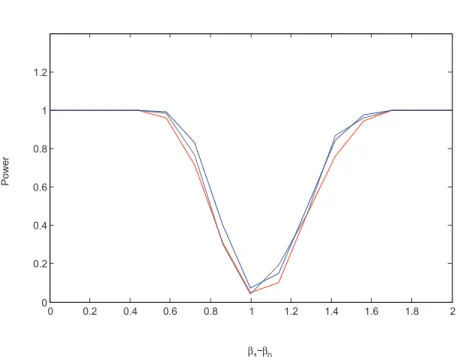
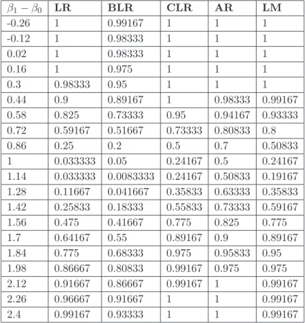
First, correctly specified model is generated for the sample of n = 200 and with weak instruments (π∗TZZTπ∗ = C
n). In this case powers of TBLR, TCLR and true TLR tests are drawn on the figure
(8.1). To be consistentTBLRis also compared toTLM andTAR. The comparison is given on the figure (8.2) and the data in the case is aggregated in the table (1).
Moreover an important step is to check how robust TBLR to a misspecification of the model. Three
koziuk, a. 18
1. ε1,ε2 ∼Laplace(0,1), 2. ε1i,ε2i∼ N(0,5niΩ),
3. ε1i,ε2i∼ N(0,(2 + 1.5 sin(6πi/n))Ω).
Experiment (1) can be found on the figure (8.3), (8.4) and in the table (2). Numerical study of the experiment (2) with misspecified heteroskedastic error is given on the figure (8.5) and is collected in the table (3). The last experiment is shown on the figure (8.6) and in the table (4).
On practice one wants to distinguish instruments based on its strength. For the clarity of exposition the section considers a simplified log-likelihood (2.19) identifying complete model with the Fisher information matrix D20 =−ΔIEL(θ∗) = n i=1 K k=1 IEη∗kiη∗kiT = n i=1 K k=1 IEWikΨ(Xi)ΨT(Xi)Wik.
Weak instrumental variables introduce an unavoidable lower bound on estimation error (lemma [7.1], see the proof in the appendix (8.1)).
Lemma 7.1. Let conditions (4.1) hold then
∃N >0, s.t. ∀n > N IEθ−θ∗2 ≥ CJ supu=1 n i=1 K k=1 IEuTΨ(X i)Wik 2,
with a factorCJ >0depending on dimensionality J.
In view of a hypothesis testing it amounts to an indifference region of a test (see the section ’Numer-ical’).
Classification of Instrumental Variables: 1. Weak instruments sup u=1 n i=1 K k=1 IEuTΨ(Xi)Wik 2 ∼K/C and IEθ−θ∗2≥ CCJ K 2. Semi-strong instruments with 0< α <1
sup u=1 n i=1 K k=1 IEuTΨ(Xi)Wik2∼Knα/C and IEθ−θ∗2 ≥ CCJ Kn1−α 3. Strong instruments sup u=1 n i=1 K k=1 IEuTΨ(Xi)Wik2∼Kn/C and IEθ−θ∗2≥ CCJ Kn
Weak instruments effectively cancel an analysis based on a limiting distribution of a test statistics. Therefore, an IV regression requires a treatment under the finite sample assumption.
8
Appendix
8.1
Classification of instrumental variables
Lemma 8.1. Let conditions (4.1) hold then∃N >0, s.t. ∀n > N IEθ−θ∗2≥ CJ supu=1 n i=1 K k=1 IEuTΨ(X i)Wik 2,
with a factorCJ >0 depending on dimensionalityJ.
Proof. Fisher expansion (Spokoiny [17]) on the set of dominating probability IP(Υ) > 1−Ce−x is written as
D0
θ−θ∗−ξ ≤C(J+x)/√n. with the matrixD20=
n i=1 K k=1 IEWk
i Ψ(Xi)ΨT(Xi)Wik. Introduce also an inequality
ξ2≤ξ−D0 θ−θ∗+D0θ−θ∗2≤2ξ−D0θ−θ∗2+ 2D0θ−θ∗2. It gives IED0(θ−θ∗)2 ≥IEΥD0(θ−θ∗)2≥ 1 2IEΥξ 2−C(J+x)2/n
and the inquired statement follows withN >0 s.t. infN{12IEΥξ2−C(J+x)2/N >0}and a constant
CJ def= 1
2IEΥξ2−C(J+x)2/N.
8.2
Non-parametric bias
The bias term - bJ def= θ−θ∗ - between parametric and non-parametric functions from the model in chapter 2 is quantified in the lemma.
Lemma 8.2. Assume that basis functions ψj follow
-(s2)
j ≤js2ψj
with some positive constantss1, s2, s3. Let f(x) be s.t. f ∈ Ss where
Ssdef= {f :||Dsg|| ≤C f},
with the notationDs(·)def= ∂∂xs1∂∂ws2 ∂∂zs3(·) forsi=1:3 ≤s. Then bias satisfies
P roof :
Straightforwardly using smoothness of functions from a Sobolev class it can be argued for s <∞that -Jsθ∗−θ∗=Js j θ∗jψj− j≤J θj∗ψj ≤ j θj∗jsψj ≤ Dsf ≤Cf and the result follows.
End of P roof
8.3
Re-sampled quasi log-likelihood
A basis for the statistical investigation of a re-sampled log-likelihood builds on the probabilistic equiv-alence with an original quasi log-likelihood. In the section one also uses notations from Spokoiny 2012 [17].
An analogue to (ED0) condition for re-sampled log-likelihood - will be referred to as (EDB0) -readily follows from normality of re-sampling weights {ui}i=1,n.
Lemma 8.3. Suppose that conditions (4.1) are justified, then there exist a positive symmetric matrix V0 and constants ν0≥1 and g≥0 such thatVar (∇ζ(θ∗))≤V02 and
∀γ= 1 logIEexp λγ T∇ζ(θ∗) V0γ ≤ ν02λ2 2 , |λ| ≤g with probability ≥1−e−x.
Proof. Define a vector
sidef= ∇i(θ ∗)
V0γ , then using normality of re-sampling weightsui rewrite
logIEexp λγ T∇ζ(θ∗) V0γ = logIEexp λ V0γ γT n i=1 ∇(Yi,θ∗)(ui−1) = = logIEexp n i=1 λγTsi(ui−1) ≤ ν02λ2 2 n i=1 γTsi2≤ ν 2 0λ2 2 , where ν0 def= ν2
0+Cδ for some positive constant C >0 and small δ. The last inequality is derived
using
n
i=1
γTsi2≤1 +Cδfrom definition ofV0and matrix concentration inequality (thm [8.20]). Re-sampling analogue to the condition (ED2) (Spokoiny 2012 [17]) also follows.
koziuk, a. 22
Lemma 8.4. Let conditions (4.1) hold true then there exist a positive valueω1(r)def=
4ν2 0ω2x+
2Cδ2(r)
n
and for each r≥0, a constantg(r)≥0such that it holds for any v∈Υ(r) logIEexp λ ω1(r) γT1∇2ζ(θ∗)γ2 D0γ1 D0γ2 ≤ ν02λ2 2 , |λ| ≤g(r).
Proof. Here it is convenient to reformulate conditions (L) and (ED2). Bound on deterministic co-variance structure can be rewritten as
D−01(D2(θ)−D02)D−01=D−01(− n i=1 ∇2IE(Y i,θ)−D20)D−01= = n i=1 (D−01∇2IE(Yi,θ)D−01+ Ip n)=nD −1 0 ∇2IE(Yi,θ)D−01+ Ip n ≤δ(r), and it follows D−01∇2IE(Yi,θ)D−01 ≤ Cδ(r) n .
Next, rewrite (ED2) mostly in the same fashion, so that it is capable to quantifyD−01∇2ζ
i(θ)D−01. It follows logIEexp{λ ω γT 1∇2ζ(θ)γ2 D0γ1 D0γ2} = logIEexp{λ ω n i=1 γT 1∇2ζi(θ)γ2 D0γ1 D0γ2} = =nlogIEexp{λ ω γT1∇2ζi(θ)γ2 D0γ1 D0γ2} ,
where ζi(v) = (Yi,θ)−IE(Yi,θ). This means that component-wise (ED2) condition holds true, namely that sup γ1,γ2∈IRp logIEexp{λ ω γ1T∇2ζi(θ)γ2 D0γ1 D0γ2} ≤ ν02λ2 2n , |λ| ≤g(r).
The two constitute the substance of the proof. Define complementary variables si def= γ1T∇2(Yi,θ)γ2
D0γ1 D0γ2 and rewrite logIEexp{ λ ω1(r) γT 1∇2ζ(θ)γ2 D0γ1 D0γ2} = logIEexp{ n i=1 λ ω1(r)si(ui−1)} ≤ ν2 0λ2 2ω2 1(r) n i=1 s2i.
To claim the statement it is sufficient to limit sum
n
i=1
s2i. Once again rewrite this sum using mentioned above (L) -n i=1 s2i = n i=1 γT 1∇2ζi(θ)γ2 D0γ1 D0γ2 + γ T 1∇2IE(Yi,θ)γ2 D0γ1 D0γ2 2 ≤ ≤2 n i=1 γT1∇2ζi(v)γ2 D0γ1 D0γ2 2 + 2 n i=1 γ1T∇2IE(Yi,θ)γ2 D0γ1 D0γ2 2 ≤