Implied Volatility Measures
Markus Yli-Niemi
August 28, 2018
Bachelor’s Thesis,
Aalto University School of Business, Department of Economics
AuthorMarkus Yli-Niemi
Title of thesisImplied Volatility Measures DegreeBachelor of Science
Degree programmeEconomics
Thesis advisor(s)Pauli Murto & Mikko Mustonen
Year of approval2018 Number of pages25+3 LanguageEnglish
Abstract
In this thesis the construction of implied volatility measures is considered. Two popular option pricing models, namely Black-Scholes model and Cox-Ross-Rubinstein binomial model, are derived, solved and their inversion is considered to obtain implied volatility estimates. In addition, current market volatility indexes used by practitioners are discussed and Chicago Board Options Exchange’s (CBOE) VIX index is derived in detail.
Implied volatility measures rely heavily on the underlying assumptions of the option pricing models. In this thesis we assume the underlying asset to follow the geometric Brownian motion. The geometric Brownian motion is derived and the implications of the motion are discussed. Also, other assumptions in the pricing models are discussed.
Due to some unrealistic assumptions in the pricing models, implied volatility measures have limitations and problems. These problems are introduced and the ways to alleviate these problems are discussed.
KeywordsImplied volatility, CBOE VIX index, Black-Scholes model, Cox-Ross-Rubinstein binomial model
Contents
1 Introduction 2
2 Geometric Brownian motion as underlying asset’s price process 5
3 Option pricing models 8
3.1 Black-Scholes model . . . 8 3.2 Cox-Ross-Rubinstein binomial model . . . 11
4 Implied volatility 15
4.1 Term structure of implied volatility and implied volatility smile . 16 4.2 Implied volatility measures and indexes . . . 18 4.3 CBOE’s VIX index . . . 19
5 Conclusion 23
6 References 24
1
Introduction
In many applications of economics and finance volatility is in the central role. Volatility is the standard deviation of a time-series, such as price process, trad-ing volume or temperature of a city, and therefore it measures how prone process is for changes, i.e. how volatile is the process we are examining. It is easy to find applications for volatility in finance such as predicting market movements or hedging portfolio, but volatility can also be used in other fields of economics, for example if we consider warehouse manager managing inventory in some industrial organization, by having idea of the volatility of inventory demand warehouse manager can retain desired inventory levels.
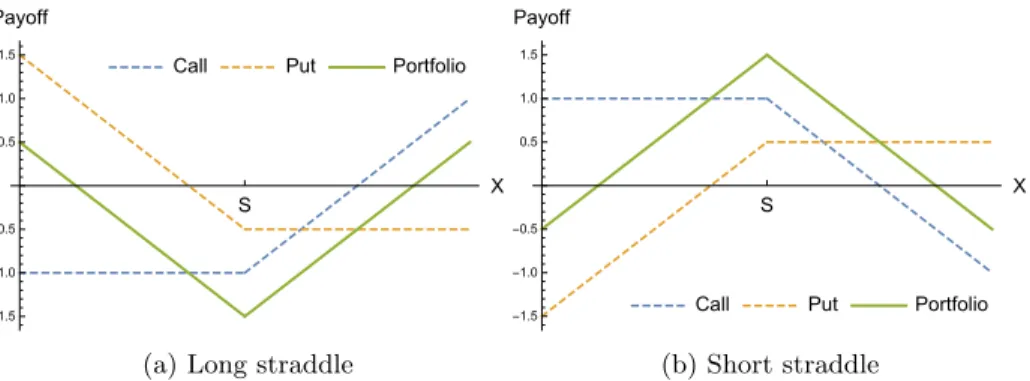
Let us consider one example application of volatility in detail. Suppose we are portfolio managers and we would like to cash in with our expectation of the future volatility of a stock whose price with respect to timetis denoted byX(t). One way to do this is to construct a straddle portfolio as depicted in Figure 1. If we expect that the volatility is large, i.e. the stock price X is expected to deviate significantly from the strike priceS, we can buy one call option and one put option with the strike priceS, which yield a payoff shown by the green curve in Figure 1 (a). Then again if we expect that the volatility is small, i.e. the stock priceX remains close to the strike priceS, we can write one call option and one put option with the strike priceS, which yield a payoff shown by the green curve in Figure 1 (b). If our expectation of the future volatility is correct and the stock priceX does not experience abrupt change, we will earn positive profits on our strategies.
So how would we construct our estimate of the future volatility? One obvi-ous way is to take historical values of our time-series, calculate the standard deviation for the historical values and use the result as an estimate for the future volatility. This estimate is called historical volatility and is one of the simplest methods to construct an estimate for the future volatility, and probably accurate in some applications such as managing inventory levels if the future volatility follows past volatility. But in the case of financial markets, literature has shown that the historical volatility is not a good estimate for the future volatility (see e.g. [1], [2]). This means that in financial markets we need to find other ways to estimate the future volatility.
To approach the issue of finding better volatility estimates for financial mar-kets one could turn to products that are traded in financial marmar-kets and ask whether there are some products that would contain information about the fu-ture volatility. Fortunately for us, the answer for this question is yes, and these products are called options. In derivatives markets, option prices follow closely prices implied by option pricing models that take the future volatility as one of the input arguments and output the value of option at timet[3]. Because option prices are observable from the derivatives markets in real time, we can invert the option pricing models to find what is the level of volatility that would yield
Call Put Portfolio S X -1.5 -1.0 -0.5 0.5 1.0 1.5 Payoff
(a) Long straddle
Call Put Portfolio S X -1.5 -1.0 -0.5 0.5 1.0 1.5 Payoff (b) Short straddle
Figure 1: Straddle strategies
the current market price of options. This estimate of volatility is called implied volatility and it measures the expected level of volatility market participants have on underlying asset.
The powerful feature of implied volatility is that it can be computed to all as-sets that have options written on them. This means we can calculate implied volatilities to securities (such as stocks and commodities), derivatives (such as futures) and indexes (such as S&P 500), and use these estimates to construct combined volatility estimates (such as volatility estimates for specific industry). Also, the idea of calculating implied volatilities is simple, which makes it easily applicable estimate for volatility.
Due to the beneficial properties of implied volatility, it has been widely adopted in the financial markets. Option markets around the world provide volatil-ity indexes that are based on calculating implied volatilities, and one of the most well-known and cited such indexes is VIX index by Chicago Board of Op-tions Exchange (CBOE) [4]. In addition to providing volatility indexes, option markets provide derivatives (futures and options) on volatility indexes, making volatility a tradable asset.
To illustrate the need for derivatives on volatility, or tradable products on volatility in general, we can return back to our example where we acted as portfolio managers trying to cash in with our expectation on the future volatil-ity. To bet on volatility, we used straddle strategies, which would profit us in case our volatility expectation turned out to be correct and the stock price did not experience abrupt changes. But what if it was the case that in one day, let say due to an earnings release, the stock price experienced an offset in price (either positive or negative) and after the offset, stock remained to have fluctuations around that new price level as it used to have around the price level before earnings release. In this example volatility remained the same but the stock price is now away from the strike price which would affect the payoff of our straddle strategy. Therefore in a straddle, we are exposed on the price
level of the underlying asset besides the volatility. In volatility products, price level effects are eliminated and we are only exposed on changes in the volatil-ity (more applications for volatilvolatil-ity products can be found for example from [5]). Although implied volatility has many beneficial properties, it also has major disadvantages and shortcomings. The most imminent problem is that option pricing models that are used to calculate implied volatilities are based on as-sumptions that are not true in real markets. This causes the real price of options differ from theoretical values implied by option pricing models, and while price differentials are generally small, as discussed earlier, the sensitivity of implied volatility to the option price (also known as the reciprocal of vega) can be large and therefore can cause large deviations in implied volatility estimates. Because basically all option pricing models are based on some form of arbitrage argu-ment (i.e. all riskless strategies yield risk-free return), the implied volatility is correct estimate of future volatility only if financial markets are efficient and other assumptions of option pricing models are correct (i.e. option pricing mod-els correspond exactly to real-life markets).
In this thesis, I aim to introduce reader to implied volatility measures by intro-ducing the two most important option pricing models, known as Black-Scholes model [6] and Cox-Ross-Rubinstein (CRR) binomial model [7], [8], alongside the assumptions of these models, how these models are inverted to find implied volatility measures, and how these models lead to volatility indexes used in real markets, such as CBOE’s VIX index. Even though implied volatility indexes have proven to have significant importance in financial markets, it is important that reader understands the assumptions behind these volatility measures and the disadvantages that are implied by these assumptions.
One of the most crucial assumptions in option pricing models is the process that the underlying asset’s price is assumed to obey. The most popular price process is a geometric Brownian motion which is also used in Black-Scholes model, Cox-Ross-Rubinstein binomial model, and in VIX index. Therefore we will start by introducing reader to the geometric Brownian motion and what type of characteristics it implies to the price process.
2
Geometric Brownian motion as underlying
as-set’s price process
Consider a deterministic system dxdt(t) =x(t)∗b(x(t))⇔dx(t) =x(t)∗b(x(t))dt in integral form:
x(t)−x(0) =
Z t
0
x(s)∗b(x(s))ds. (2.0.1)
Suppose the process has random element (i.e. noise) that is modelled asσBt,
where σ denotes volatility and process B = (Bt)t∈R+ is a standard Brownian motion (stdBM). We can write (2.0.1) as a stochastic process:
Xt−X0= Z t
0
Xs∗b(Xs)ds+σBt, (2.0.2)
where Xt =X(t) denotes the price of the underlying asset at time t. Let us
modelσas a function of the processX, i.e. σ(X). We get from (2.0.2):
Xt−X0= Z t 0 Xs∗b(Xs)ds | {z } =drift + Z t 0 σ(Xs)dBs | {z } =noise . (2.0.3)
In the differential form (2.0.3) is:
dXt=Xt∗b(Xt)dt+σ(Xt)dBt. (2.0.4)
By denotingb(Xt) =µand assuming thatσ(Xt) =σXt, (2.0.4) simplifies to:
dXt=µXtdt+σXtdBt. (2.0.5)
Equation (2.0.5) is the differential form of geometric Brownian motion (also known as geometric SDE) that is used to model the price of asset with respect to time t. It is composed of a drift which determines the price level of the process, and a noise which determines the level of fluctuation around the price level of the process.
To find a solution to the geometric Brownian motion, we write (2.0.5) in the integral form: Z t 0 dXs Xs = Z t 0 µds+ Z t 0 σdBs=µ Z t 0 ds+σ Z t 0 dBs=µt+σBt. (2.0.6)
differentiable. Also the price processX is a semimartingale because it can be decomposed into a finite variation process (drift in this case) and a martingale (noise in this case, stdBM is a martingale). Thus we can use Ito’s formula (see Theorem 3.22 in [9]): f(Xt)−f(X0) = Z t 0 f0(Xs)dXs+ 1 2 Z t 0 f00(Xs)dhX, Xis ⇔ln (Xt)−ln (X0) = Z t 0 1 Xs dXs−1 2 Z t 0 1 X2 s dhX, Xis (2.0.7) ⇒d(ln (Xt)) = dXt Xt − 1 2 1 X2 t dhX, Xit (2.0.8)
In (2.0.7) and (2.0.8) we need to solve the quadratic variationhX, Xit. To do
this we first introduce an integral processH rM = ((H rM)
t)t∈R+, where (H rM) t is defined as: (H rM) t= b2nt c X k=1 H(k−1)2−n Mk2−n−M(k−1)2−n. (2.0.9) Notice that (H rM) t n→∞
−→ R0tHsdMs. Quadratic variation of the integral process
is introduced as Theorem 3.12 in [9] and reads:
hHrM, H rM
it= Z t
0
Hs2dhM, Mis. (2.0.10)
NowhX, Xitcan be written as (denote time by T):
hX, Xit=h(µX)rT,(µX)rTi t+h(σX)rB,(σX)rBi t = Z t 0 µ2Xs2dhT, Tis+ Z t 0 σ2Xs2dhB, Bis ∗ = Z t 0 σ2Xs2ds ⇒dhX, Xit=σ2Xt2dt. (2.0.11)
(*) We used the fact that hT, Tit = 0 for finite variation processes, and time
T is a finite variation process. Quadratic variation of the standard Brownian
motionhB, Bit=t.
ln (Xt)−ln (X0) = Z t 0 1 Xs dXs− 1 2 Z t 0 1 X2 s σ2X2 sds (2.0.12) ⇔ln X t X0 = Z t 0 1 Xs dXs | {z } =µt+σBt −12σ2t= µ−1 2σ 2 t+σBt. (2.0.13)
Taking exponential of (2.0.13) gives the solution of the geometric SDE: Xt=X0e(µ−
1 2σ
2
)t+σBt. (2.0.14)
Solution (2.0.14) can be written as: ln (Xt) = ln (X0) + µ−1 2σ 2 t | {z } deterministic +σ Bt |{z} ∼N(0,t) (2.0.15) Thus ln (Xt)∼ N µ,¯ σ¯2
, where ¯µand ¯σ2 are given as:
¯ µ=E[ln (Xt)] = ln (X0) + µ−1 2σ 2 t, (2.0.16) ¯ σ2= Var [ln (X t)] = Var [σBt] =σ2t. (2.0.17)
We say that Xt obeys a log-normal distribution because ln (Xt) (i.e. the log
price) is normally distributed. The variance of log price depends on timetand volatility parameterσwhich is assumed to be constant by the equation (2.0.5). The assumption thatσis constant means that in later sections when we derive implied volatility estimates forσwe should get the same estimate regardless of the strike price and the time-to-maturity of option as long as the underlying asset is the same. However, implied volatility estimates will differ depending on the time-to-maturity and the strike price of option [10], referred as the term structure of volatility and the volatility smile, respectively. These issues will be discussed in detail in later sections.
Now, as we have introduced the process the price of underlying asset obeys we can move on to derive the Black-Scholes and CRR-binomial tree option pric-ing models. In next two sections we will derive these models and show how they can be used to calculate implied volatility estimates for underlying assets.
3
Option pricing models
In this section we aim to derive the two most common option pricing models, namely Black-Scholes model and CRR-binomial model. We will do derivations in detail to provide the reader with thorough understanding of these models before moving on to the implied volatility measures. Good understanding of these option pricing models is a prerequisite to fully understand the implied volatility measures.
To begin, let us introduce assumptions that we will use in the derivation of Black-Scholes and CRR-binomial models:
(i) Short-term interest rate is known and constant.
(ii) Underlying asset’s price processX = (Xt)t∈R+ is a geometric Brownian motion.
(iii) Underlying asset pays no dividend or other distribution.
(iv) OptionV(X, t) is an European option, i.e. executable only on the maturity date.
(v) There are no transaction costs.
(vi) We can buy and sell any fraction of the underlying asset.
(vii) Markets are efficient, i.e. riskless profit opportunities yield the risk-free interest rate.
Assumptions (iii) and (iv) can easily be relaxed, i.e. we could allow the under-lying asset to pay distributions and we could consider American options instead of European options, but for the sake of simplicity we will stick to these two assumptions. The idea of analysis does not differ whether we allow asset to pay distributions or whether we consider American options instead of European options.
3.1
Black-Scholes model
To derive Black-Scholes model, let us begin by considering portfolio consisting of one stock (or could be any other asset that has options written on it) with the priceX(t) at timet, and call options with value (or payoff)V(X, t) to underlying stock. We want to delta-hedge this portfolio, meaning that the value of the portfolio remains unchanged when small change in the stock priceX happens. If the change in stock price, denoted by ∆X, is small we can approximate the change in the value of option ∆V by the first-order Taylor expansion:
dV =V(X+dX, t)−V(X, t) = ∂V
Because the value of the call option increases as the stock price increases, i.e.
∂V
∂X >0, a long position in stock requires a short position in call option to obtain
a delta-hedged portfolio. The value of the portfolio, denoted byW(X, V(X, t)) is:
W(X, V(X, t)) =X−KV(X, t), (3.1.2)
whereK∈Ris the number of call options in the delta-hedged portfolio. To have a delta-hedged position, small change in the price of the stock should not change the value of the portfolio. Thus the number of call options in the portfolio is:
W(X+ ∆X, V(X+ ∆X, t))−W(X, V(X, t)) =X+ ∆X−KV(X+ ∆X, t)−X+KV(X, t) = ∆X−K(V(X+ ∆X, t) +V(X, t)) = 0 ⇒K(V(X+ ∆X, t)−V(X, t)) = ∆X ⇔K∂V ∂X∆X = ∆X ⇒K= 1 ∂V ∂X . (3.1.3)
Thus the value of the portfolio (also called the equity) at timet is: W(X, V(X, t)) =X− 1
∂V /∂XV(X, t). (3.1.4) The change of the portfolio value with respect to small time stepdtis:
dW =dX− 1
∂V /∂XdV, (3.1.5)
where the change in call options value can be written using Ito’s formula (see Theorem 3.22 in [9]): V(X+dX, t+dt)−V(X, t) = Z τ+dτ τ ∂V ∂XdXs+ Z τ+dτ τ ∂V ∂t ds+ 1 2 Z τ+dτ τ ∂2V ∂X2dhX, Xis+ Z τ+dτ τ ∂2V ∂X∂tdhX, tis+ 1 2 Z τ+dτ τ ∂2V ∂t2 dht, tis ∗ = Z τ+dτ τ ∂V ∂XdXs+ Z τ+dτ τ ∂V ∂t ds+ 1 2 Z τ+dτ τ ∂2V ∂X2σ 2X2 tds = Z τ+dτ τ ∂V ∂XdXs+ Z τ+dτ τ ∂V ∂t + 1 2 ∂2V ∂X2σ 2X2 t ds ⇒dV = ∂V ∂XdXt+ ∂V ∂t + 1 2 ∂2V ∂X2σ 2X2 t dt. (3.1.6)
(*) We assume the stock price obeys geometric Brownian motion. ThusdhX, Xit=
σ2X2
tdt. Also the quadratic variation of finite variation processes is zero.
By substituting (3.1.6) to (3.1.5) we get the change of the portfolio value with respect to time: dW =dX− 1 ∂V /∂X ∂V ∂XdXt+ ∂V ∂t + 1 2 ∂2V ∂X2σ 2X2 t dt =−∂V /∂Xdt ∂V ∂t + 1 2 ∂2V ∂X2σ 2X2 t . (3.1.7)
Because the value of the delta-hedged portfolio is independent of the stock price, it has no risk. Therefore the return dW must equal the risk-free interest rate rf (this is the arbitrage argument of Black-Scholes model):
dW =− dt ∂V /∂X ∂V ∂t + 1 2 ∂2V ∂X2σ 2X2 t =W ∗rfdt= Xt− 1 ∂V /∂XV(X, t) ∗rfdt ⇒ −∂V /∂X1 ∂V ∂t + 1 2 ∂2V ∂X2σ 2X2 t =rfXt−rf 1 ∂V /∂XV(X, t) ⇒∂V∂t =rfV(X, t)−rfXt∂V ∂X − 1 2σ 2X2 t ∂2V ∂X2. (3.1.8)
The stochastic differential equation (3.1.8) is called the Black-Scholes equation for the value of a call option. By denoting the maturity date (or expiration date) of the option byT and the execution price (or strike price) byS, we can write boundary conditions for (3.1.8):
V(0, t) = 0,∀t∈[0, T] (3.1.9a) V(Xt, t) Xt→∞ −→ Xt (3.1.9b) V(XT, T) = max{XT −S,0} (3.1.9c)
To solve (3.1.8) with the boundary conditions (3.1.9a)-(3.1.9c) we will transform (3.1.8) to an ordinary diffusion equation with a change of variables and solve this diffusion equation with its Green’s function (this is done in Appendix A). This procedure yields solution:
where Ψ(•) is the cumulative distribution function (CDF) of the standard nor-mal distribution andd±(τ, x) =
ln(Xt/S)+(rf±12σ 2)
τ
σ√τ , τ =T −t. To price put
options we use the put-call parity which makes (3.1.10) applicable also in the pricing of put options.
3.2
Cox-Ross-Rubinstein binomial model
Consider a stock with the price Xk, k ∈ Z+ at state k. In state k stock can
either go up or down. The most simple such system has k∈ {n, n+ 1} and is called a two state system.
Let us consider a portfolio that buys H stocks (H also called hedging ratio) and sells one call option with the strike price S. Option is maturing at the ending state of the system (in two state system whenk=n+ 1). By denoting the value of the option byV, the initial investment in the statek=nand the payoff in maturity (statek=n+ 1):
k=n:Wn =HXn−Vn (3.2.1) k=n+ 1 :Wn(up)+1 =HX (up) n+1−max n Xn(up)+1 −S,0 o OR Wn(down)+1 =HX (down) n+1 −max n Xn(down)+1 −S,0 o . (3.2.2)
Now let us findH such that the payoff for the portfolio in the maturity is the same regardless of the price of the stock in the maturity:
Wn(up)+1 =W (down) n+1 ⇒HX (up) n+1−max n Xn(up)+1−S,0 o =HXn(down)+1 −max n Xn(down)+1 −S,0 o ⇒H= max n Xn(up)+1−S,0 o −maxnXn(down)+1 −S,0 o Xn(up)+1−X (down) n+1 . (3.2.3)
With the hedge ratio given by (3.2.3) portfolio’s payoff in the maturity does not depend on the price of the stock, therefore we have a certain (i.e. riskless) payoff. For a riskless payoff investors require the risk-free interest rate rf (this is the
arbitrage argument of binomial models). By continuous interest compounding we have:
Wn=Wn+1e−rfT, (3.2.4)
day, week, month, etc.). By substituting (3.2.1) and (3.2.2) to (3.2.4) we obtain the price of the call option in staten:
HXn−Vn=
HXn(up)+1−maxnXn(up)+1 −S,0oe−rfT
⇒Vn=HXn−
HXn(up)+1 −maxnXn(up)+1−S,0oe−rfT. (3.2.5)
For multiple state systems, we use the two-state model starting from the last two states (i.e. maturity state and state before maturity) and backpropagate the result all the way to the first node.
Alternative approach, which yields exactly the same result as the method above, to value options in 2-state system is to consider the probability for the stock price moving up, denoted by pu. Let us determine pu such that the expected
payoff from the stock is the same now and in the next state, i.e.:
Xn=E[Xn+1]⇔Xn =puXn(up)+1 + (1−pu)Xn(down)+1 . (3.2.6)
A risk neutral person is indifferent of selling the stock now or selling it in the next state if the portfolio yields a risk-free return:
Xn=E[Xn+1]e−rfT ⇔Xn= puXn(up)+1 + (1−pu)Xn(down)+1 e−rfT. (3.2.7) This givespu: pu= XnerfT−Xn(down)+1 Xn(up)+1−X (down) n+1 . (3.2.8)
Usingpu we can write the value of the optionV:
Vn=E[Vn+1]e−rfT = puVn(up)+1 + (1−pu)Vn(down)+1 e−rfT =pumax n Xn(up)+1−S,0 o + (1−pu) max n Xn(down)+1 −S,0 o e−rfT. (3.2.9) The problem with binomial option pricing is that we need to predetermine the price of the stock in each state of the systemk∈Z+. One way to overcome this issue is to use a stochastic price movement, which is the idea in CRR-binomial model.
by ln (Xn). Now in CRR-model the log-price can either increase by ln(u) or
decrease by ln(d). This implies possible price movements:
lnXn(up)+1 = ln (Xn) + ln(u)⇒Xn(up)+1 =Xn∗u (3.2.10) lnXn(down)+1 = ln (Xn)−ln(d)⇒Xn(down)+1 =Xn∗d. (3.2.11)
Next step is to determine u and d. By substituting (3.2.10) and (3.2.11) to (3.2.8) we get the probability of up movement:
pu=
erfT −d
u−d . (3.2.12)
In a risk neutral world, we also require that the volatility of portfolios are the same, not only the expected returns. By assuming a small time step between statesnandn+ 1 (i.e. T is small), we can approximate:
Var (Xn+1)=∗ Xn2e2µT eσ2T −1 ** ≈Xn2(1 + 2µT)σ2T =Xn2 σ2T+ 2µσ2|{z}T2 ≈0 ! ≈Xn2σ2T (3.2.13)
(*) By assumption (ii),ln (Xn+1)∼ N µ,¯ σ¯2, whereµ¯= ln (X0) + µ−12σ2t and¯σ2=σ2t. Thus Var(X
n+1) =Xn2e2µT eσ2 T −1. (**) For smallx,ex ≈1 +x.
By using the approximation of Var (Xn+1), we get:
Var (Xn+1)) | {z } ≈X2 nσ2T =EXn2+1 −E[Xn+1]2 =puu2Xn2+ (1−pu)d2Xn2−(puuXn+ (1−pu)dXn)2 ⇔Xn2σ2T =puu2Xn2+ (1−pu)d2Xn2−p2uu2Xn2− 2pu(1−pu)udXn2−(1−pu)2d2Xn2 ⇒σ2T =puu2+ (1−pu)d2−p2uu2−2pu(1−pu)ud−(1−pu)2d2 = pu−p2u (u−d)2. (3.2.14)
By substituting (3.2.12) to (3.2.14), we get: σ2T = (u−d) e rfT−d− erfT −d2 (u−d)2 (u−d) 2 = (u−d) erfT −d− erfT−d2 =uerfT −ud−derfT +d2−e2rfT + 2erfTd−d2 = (u+d)erfT −ud−e2rfT. (3.2.15)
CRR-method assumes thatd=u1. By substituting this into (3.2.15) we get:
σ2T = u+ 1 u erfT −1−e2rfT ⇒u+1 u=e −rfT σ2T+ 1+erfT ≈(1−rfT) σ2T+ 1 + (1 +rfT) =σ2T+ 1−σ2rf T2 |{z} ≈0 −rfT+ 1 +rfT = 2 +σ2T ⇒u2 − 2 +σ2Tu+ 1 = 0 ⇒u= 2 +σ 2T±q(2 +σ2T)2−4 2 = 2 +σ2T ±√4 + 4σ2T+σ4T2−4 2 = 2 +σ 2T±2√σ2T 2 = 1 + σ 2T 2 | {z } σ√T ±σ√T u≥1 = 1 +σ√T ≈eσ√T. (3.2.16)
We obtainedu=eσ√T and respectivelyd= 1
u =e−σ
√
T in Cox-Ross-Rubinstein
method. It is important to keep in mind that in CRR-method we assume a small time step between states, i.e. T is small. It is worth noting that consecutive up and down movements will cancel each others, i.e. d∗u= 1.
Now, as we have derived the two most common option pricing models along with their assumptions, we are ready to construct implied volatility measures. In the next section we will show how implied volatility measures are computed from option pricing models and how these relate to volatility indexes used in markets such as CBOE’s VIX index. Also, we will discuss in detail the problems and shortcomings of implied volatility measures, which are important to keep in mind when using implied volatility measures in practise.
4
Implied volatility
As we saw in the sections 3.1 and 3.2, where we derived Black-Scholes and CRR-binomial option pricing models, volatilityσof the underlying asset was one of the inputs that we used in the option pricing models to determine the value of a option at timet. In both of these models, volatilityσ was introduced in the noise term of the geometric Brownian motion, which resulted in the stock price to be log-normally distributed. This assumption yielded closed-form solution for option price in Black-Scholes model, and deterministic up (u=eσ√T) and
down (d=e−σ√T) movements in CRR-binomial tree.
One challenge in option pricing models is that volatility of underlying asset is not directly observable from the market, as is the case for the other parameters of these two models, i.e. the price of the stockX, the risk-free interest raterf,
the time-to-maturityT and the option priceV orP (call and put respectively). Therefore, because we have only one unknown variable in our model, namely volatility, option pricing models such as Black-Scholes and CRR-binomial tree can be used to find the volatility. This is done by inverting the option pricing model to find the volatility of the underlying asset such that the option pricing model gives the correct price of the option. The volatility resulting from the option pricing model inversion is called implied volatility.
To be more precise, let us denote the option pricing model by function f : (σ,Ω) → V, where Ω denotes the set of input parameters of the option pric-ing model besides volatility σ. Thus the option pricing model can be seen as a function f that gets inputs, in which volatility σ is one of the arguments, and outputs the price of the option V. Because we find values of V and Ω from the markets we can find the implied volatility σ by the inverse function f−1 : (V,Ω)
→ σ. This is how we theoretically find the implied volatility by using option pricing models such as Black-Scholes and CRR-binomial tree. Although it is theoretically simple to find implied volatilities, practically it is more challenging, because in general case there is no closed-form expression for the inverse function f−1 (in certain cases it is possible to find a closed form
solution for f−1 by using approximations, see e.g. [11]). If we do not have
closed form expression for the inverse function, we can find the implied volatil-ity numerically by solving a root finding equation:
f(σ,Ω)−V = 0. (4.0.1)
Equation (4.0.1) can be solved with any root finding method, such as Newton’s method, Quasi-Newton’s methods (e.g. secant method), Bisection or some other fixed point iteration schemes. It is important to notice that some root finding algorithms work better than the others depending on the option pricing model we use to find the implied volatility. For example, when using Black-Scholes
model it is convenient to use Newton’s method because there is closed form expression for ∂f∂σ, but in the case of CRR-binomial model computation of ∂f∂σ is costly because closed from expression does not exist and finding the derivative requires lengthy chain rule expressions (similar phenomena as in neural net-works). If we want to find implied volatilities in real-time it is important to choose the root finding algorithm appropriately.
As we now know how to calculate implied volatilities by inverting option pric-ing models or solvpric-ing equations of form (4.0.1) by root findpric-ing algorithms, next step is to use implied volatilities to construct implied volatility measures and indexes. However, before moving to implied volatility measures and indexes, we need to discuss the term structure of implied volatility and implied volatility smile. These two phenomena are intrinsic part of implied volatilities and are essential to understand and keep in mind when constructing implied volatility measures and indexes.
4.1
Term structure of implied volatility and implied
volatil-ity smile
In Black-Scholes and CRR-binomial tree models we assumed that the price of the underlying assetXtfollows the geometric Brownian motion:
dXt=Xt(µdt+σdBt), (4.1.1)
where dXt = Xt−X0 denoted the price change from initial time t0 to time
t, µ was the drift parameter, σ was the volatility parameter and Bt was the
standard Brownian motion. It is important to notice that in these two option pricing models we assumedσ to be constant over time and over option strike prices. This means that when calculating implied volatilities with these option pricing models, we should get the same implied volatility regardless of the time-to-maturityT or the strike priceS of the option.
However, the empirical evidence shows that options with different time-to-maturities and strike prices have different implied volatilities (see [10]). In [10] authors had three key findings:
1. Short maturity out-of-money (i.e. for call option strike price much higher than the current stock price, for puts vice versa) calls are overpriced in the market compared to the prices predicted by Black-Scholes.
2. The price bias between the market price and the price predicted by Black-Scholes is statistically significant but the bias reverses after long periods of time.
3. None of the option pricing models up that date were able to explain that bias reversal in 2.
Because the option price increases when the volatility increases, i.e. ∂V∂σ > 0, overpriced products have higher implied volatilities than underpriced products. Thus by [10] we get the following conclusions:
(a) Short maturity out-of-money calls have higher implied volatilities than longer maturity counterparts.
(b) At-the-money calls on the first period provided higher implied volatili-ties on longer time-to-maturity options. On the second period the shorter time-to-maturity provided higher implied volatilities (trend reversal). The first period was 23.8.1976-21.10.1977 while the second period was 24.10.1977-31.8.1978.
(c) In the first period lower strike price corresponded to higher implied volatil-ity. On the second period the higher striking price corresponded to higher implied volatility.
Conclusions (a) and (b) tell that implied volatility varies over time. This is referred to as the term structure of volatility. Then again, conclusion (c) tells that the implied volatility depends also on the strike price. This is referred to as the volatility smile.
The empirical evidence by [10] shows that option prices predicted by Black-Scholes (and other option pricing models) deviate from the true market values both over time and over strike price. This means that the implied volatility changes over time and over strike price which is against the assumptions of the price process we used in the derivation of Black-Scholes model and CRR-binomial model. This can be due to two reasons: first, market imperfections (such as transaction costs) may systematically prevent option prices to take their true theoretical values or secondly, the price of the underlying asset do not follow the geometric Brownian motion with a constant volatility (i.e. our model assumptions are not correct).
To explain the term structure and smile of implied volatility, more recent option pricing models have assumed the volatility to vary over time. Widely used as-sumption in these models is to assume the volatility to follow a certain random process. This class of option pricing models is known as stochastic volatility models. One popular stochastic volatility model is Heston’s model [12] in which the underlying asset’s volatility is assumed to follow Cox-Ingersoll-Ross process [13]. In this thesis we will not discuss stochastic volatility models.
In the construction of implied volatility measures we can address the term struc-ture and smile of implied volatility by calculating implied volatilities across dif-ferent maturities and strike prices, and use a weighting scheme to calculate the final estimate of the implied volatility. Many weighting schemes are discussed in the literature, and we will shortly mention some of them in the next section.
4.2
Implied volatility measures and indexes
As was noted in the Section 4.1, options with different time-to-maturities and strike prices have different implied volatilities. Therefore it is not straightfor-ward to construct measures of implied volatilities because depending on the option type, we get different estimates for implied volatilities.
To alleviate this problem, one way to construct implied volatility measures is to find implied volatilities for options with different maturities and strike prices and then use weighted sum as the estimate of the underlying asset’s volatility. There has been many proposals in the literature of how weighting should be done. In [14] some of the most popular weighting schemes are listed and here we repeat them below:
ˆ σ= 1 N N X i=1 σ (4.2.1a) ˆ σ= PN1 i=1wi v u u t N X i=1 w2 iσ2i (4.2.1b) ˆ σ= PN i=1σi∂V∂σii σi Vi PN i=1∂V∂σii σi Vi (4.2.1c) arg min ˆ σ ( N X i=1 wi[Vi−f(ˆσ)] ) (4.2.1d)
Equation (4.2.1a) finds ˆσ as an arithmetic mean of implied volatilities of op-tions with different time-to-maturities T and strike prices S. Although this approach is simple, it does not give very accurate prediction of the implied volatility because option pricing models predict the value of options better for some combinations of T and S than others. Therefore it would make sense to put more weight on options which can be accurately priced by option pricing models. Also some options are more sensitive to volatility than others. This means that we are prone to high estimation error when estimating volatility by volatility insensitive options, and thus it would make sense to put higher weight on volatility sensitive options than insensitive ones.
Equation (4.2.1b) is suggested in [15]. The weights are chosen to bewi = ∂V∂σii
(also called vega). Equation (4.2.1c) is suggested in [16] and for weights they use option price elasticies to volatility. Equation (4.2.1d) is suggested in [2] in which author does not propose any superior way of choosing weightswi.
In market implied volatility indexes, weighting schemes of type (4.2.1a)-(4.2.1d) are used. The most followed and cited such indexes are CBOE’s VIX and RVX indexes which measure the implied volatility of S&P500 and Russell 2000 indexes
respectively, and HSI Volatility Index which measures the implied volatility of Hong Kong’s Hang Seng Index. All these indexes are calculated in the same fashion, by considering wide range of options with different maturities and strike prices and weighting the resulting implied volatilities to obtain the final value of volatility index. In the next section we will discuss CBOE’s VIX index in detail. We will discuss what is the goal of VIX index, what type of options it uses to calculate the implied volatility and how VIX index is calculated. In [4] the general form of VIX index formula is given, and we will also derive this formula.
4.3
CBOE’s VIX index
As discussed in [4], VIX index is calculated by using standard and weekly SPX (S&P 500 Index options) call and put options. Standard SPX options have monthly expiration. The SPX options that are used to calculate VIX expire on Fridays (for standard SPX options 3rd Friday of each month and weekly
SPX options expire all other Fridays). The goal of VIX index is to measure the 30-day expected volatility in S&P 500 index. CBOE uses so called near- and next-term put and call SPX options with 23 to 37 days to expiration and with wide range of strike prices (notice the term structure of volatility and volatility smile is addressed). Options expiring in 30 calendar days or less are considered near-term. Standard and Weekly SPX options are combined in VIX index to match the 30 day target time-frame as closely as possible. The composition of options and weights that are used to calculate VIX changes continuously. In VIX calculation, time-to-maturityT of options is denoted in minutes (preci-sion used by practitioners):
T = Mcurrent day+Msettlement day+Mother days
Minutes in a year , (4.3.1)
where M denotes minutes remaining until midnight on the specific date. The risk-free interest rates rf in VIX calculation are based on the U.S. Treasury
yield curve rates. The yield curve is obtained by cubic interpolation between treasury yield points to derive yields for relevant SPX options.
In [4] the general form of VIX index formula is given as: σ2= 2 T N X k=1 ∆Sk S2 k erfTQ(t, S k)− 1 T F S0 − 1 2 , (4.3.2)
where VIX-index =σ∗100,T is time-to-maturity,F is the forward index level derived from the index option prices,S0 is the first strike price below the
for-ward index levelF, Si is the strike price of the i’th out-of-money option, ∆Si
is the difference between the i’th consecutive strike prices, rf is the risk-free
the strike priceSi.
To derive (4.3.2) we assume that the log-price of the underlying asset is nor-mally distributed (as has been the convention in this thesis). We start by the identity (2.0.8) that we obtained in the Section 2 for the geometric Brownian motion: d(ln (Xt)) = dXt Xt − 1 2 1 X2 t dhX, Xit dhX,Xit=σ2Xt2dt = dXt Xt − 1 2σ 2dt. (4.3.3)
By integrating (4.3.3) from the initial time up to maturity we get:
ln XT X0 = Z T 0 1 Xs dXs | {z } =µT+σBT −12σ2T = µ−1 2σ 2 T +σBT. (4.3.4)
Taking the expected value of (4.3.4) we get:
E ln X T X0 =µT−12Eσ2T ⇒Eσ2= 2 T µT−E ln X T X0 . (4.3.5)
Next by remembering that ln (Xt)∼ N µ,¯ ¯σ2
with ¯µ= ln (X0) + µ−12σ2
t and ¯σ2 =σ2t, we can use the properties of a log-normally distributed random
variable: F=E[XT] =eµ¯+ ¯ σ2 2 =X 0e(µ− 1 2σ 2)T+1 2σ 2T =X0eµT ⇒µT= ln F X0 . (4.3.6)
By substituting (4.3.6) to the expression ofEσ2, i.e. the equation (4.3.5), we
get: Eσ2= 2 T ln F X0 −E ln X T X0 . (4.3.7)
Next we will rewrite the expected valueEhlnXT
X0
i
. By introducing a deter-ministic variableα≥0, we can write:
E ln XT X0 =E ln XT α + ln α X0 ∗ = =F z }| { E[XT] α − 1 +E Z α 0 1 S2max{S−XT,0}dS + E Z ∞ α 1 S2max{XT −S,0}dS + ln α X0 = F α − 1 + Z α 0 1 S2E[max{S−XT,0}]dS + Z ∞ α 1 S2E[max{XT−S,0}]dS + ln α X0 ** =F α − 1 + Z α 0 1 S2e rfTP(t, S)dS+ Z ∞ α 1 S2e rfTV(t, S)dS + ln α X0 *** ≈ Fα − 1 + N X k=1 ∆Sk S2 k erfTQ(t, S k) ! + ln α X0 (4.3.8) (*)R0αS12max{S−XT,0}dS= ( 0, α≤XT Rα XT 1 S2(S−XT)dS= XT α + ln α XT −1, α > XT , alsoRα∞S12 max{XT −S,0}dS= ( 0, α≥XT RXT α 1 S2 (XT−S)dS= XT α + ln α XT −1, α < XT . ⇒R0α 1 S2 max{S−XT,0}dS+ R∞ α 1 S2max{XT−S,0}dS= XαT + ln α XT −1 ⇒ln XT α = XT α − 1 + Rα 0 1 S2 max{S−XT,0}dS+ R∞ α 1 S2 max{XT−S,0}dS .
(**) By the rational pricing assumption the current price of call and put options
(V andP respectively) equals the discounted expected payoff in the maturity, i.e.
E[max{XT −S,0}] =erfTV(t, S)andE[max{S−XT,0}] =erfTP(t, S).
(***) Introduce a functionQ(t, S) =
(
V(t, S), α < XT
P(t, S), α≥XT
. Then we can write
Rα 0 1 S2erfTP(t, S)dS+ R∞ α 1 S2erfTV(t, S)dS= R∞ 0 1 S2erfTQ(t, S)dS. Denote the
ascending sequence of strike prices by{Sk}k∈{1,...,N}. Then we can approximate
the integral by R∞ 0 1 S2erfTQ(t, S)dS= PN k=1 S12 ke rfTQ(t, S k) (Sk−Sk−1) | {z } =∆Sk =PNk=1 ∆SS2k k e rfTQ(t, S k).
Thus the expression ofEσ2simplifies to: Eσ2= 2 T ln F X0 −ln α X0 −Fα+ 1 + N X k=1 ∆Sk S2 k erfTQ(t, S k) !! = 2 T ln F α −Fα + 1 + N X k=1 ∆Sk S2 k erfTQ(t, S k) !! **** ≈ T2 F S0−1− F S0 −1 2 2 − F S0 + 1 + N X k=1 ∆Sk S2 k erfTQ(t, S k) ! = 2 T N X k=1 ∆Sk S2 k erfTQ(t, S k)− F S0 −1 2 2 = 2 T N X k=1 ∆Sk S2 k erfTQ(t, S k)− 1 T F S0 − 1 2 . (4.3.9) (****) Taylor expansion: ln F α = ln 1 + F α−1 =F α−1− (F α−1) 2 2 + F α −1 3 3 −... | {z } ≈0 ≈F α−1− (F α−1) 2 2 . We have F
α ≈1if we chooseα=S0 to be the first strike price below the forward
index levelF (as was the definition in VIX formula).
In (4.3.9) we obtained the general form of VIX formula which was given in (4.3.2).
5
Conclusion
In this thesis we introduced the reader to implied volatility measures by dis-cussing how implied volatilities are calculated from option pricing models, and how implied volatility measures are used in real-life markets. We derived the most common option pricing models (i.e. Black-Scholes model and CRR-binomial model) and showed how these models are inverted to find implied volatilities. We discussed the intrinsic problems implied volatilities have (i.e. the term structure of implied volatility and implied volatility smile) and how we could alleviate these problems by considering wide range of options with different ma-turities and strike prices and constructing implied volatility measures by using a weighted sum of implied volatilities instead of the values implied by single options.
As we saw in the derivation of the option pricing models, the assumptions we make in the derivation of the model affect greatly how accurately the option pricing model values options when compared to the option prices obtained in the markets. The general setting of the option pricing models used to calculate implied volatilities is that all model parameters excluding volatility are directly observable from the markets, therefore the accuracy of the pricing model is cru-cial because it directly affects how accurate the implied volatility estimates are. As the assumptions of our pricing models affected the implied volatility esti-mates, also the market conditions had a significant effect. The option pricing models usually occupy some form of arbitrage argument which requires that risk-free profit opportunities yield the risk-free return, and the expected profit is always an increasing function of the investment riskiness in general. If this type of market efficiency does not exist in the markets the implied volatility estimates are not correct even if other pricing model assumptions correspond to the real-life scenario. Therefore it was highlighted in the thesis that our option pricing models, and thus implied volatility estimates, become inaccurate if either model assumptions are not correct or if markets are not efficient which imply that the real option prices will not converge toward their theoretical values.
6
References
[1] A. Szakmary, E. Ors, J. K. Kim and W. N. Davidson III, “The predictive power of implied volatility: Evidence from 35 futures markets,”Journal of Banking & Finance, vol. 27, no. 11, pp. 2151–2175, 2003.
[2] S. Beckers, “Standard deviations implied in option prices as predictors of future stock price variability,”Journal of Banking & Finance, vol. 5, no. 3, pp. 363–381, 1981.
[3] G. Bakshi, C. Cao and Z. Chen, “Empirical perofrmance of alternative option pricing models,” The Journal of Finance, vol. 52, no. 5, pp. 2003– 2049, 1997.
[4] Cboe Exchange, Inc., “Vix white paper - cboe volatility index,” 2018. [5] M. Brenner and D. Galai, “New financial instruments for hedging changes
in volatility,”Financial Analysts Journal, vol. 45, no. 4, pp. 61–65, 1989. [6] F. Black and M. Scholes, “The pricing of options and corporate liabilities,”
The Journal of Political Economy, vol. 81, no. 3, pp. 637–654, 1973.
[7] R. J. Rendleman and Jr. & B. J. Bartter, “Two-state option pricing,”The
Journal of Finance, vol. 34, no. 5, pp. 1093–1110, 1979.
[8] J. C. Cox, S. A. Ross and M. Rubinstein, “Option pricing: A simplified approach,” Journal of Financial Economics, vol. 7, no. 3, pp. 229–263, 1979.
[9] Nathanael Berestycki, “Stochastic calculus and applications,” 2010. [10] M. Rubinstein, “Nonparametric tests of alternative option pricing models
using all reported trades and quotes on the 30 most active cboe option classes from august 23, 1976 through august 31, 1978,” The Journal of
Finance, vol. 40, no. 2, pp. 455–480, 1985.
[11] C. J. Corrado and T. W. Miller Jr., “A note on a simple, accurate formula to compute implied standard deviations,” Journal of Banking & Finance, vol. 20, no. 3, pp. 595–603, 1996.
[12] S. L. Heston, “A closed-form solution for options with stochastic volatility with applications to bond and currency options,”The Review of Financial Studies, vol. 6, no. 2, pp. 327–343, 1993.
[13] J. C. Cox, J. E. Ingersoll, Jr. and S. A. Ross, “A theory of the term structure of interest rates,”Econometrica, vol. 53, no. 2, pp. 385–407, 1985.
[14] S. Mayhew, “Implied volatility,”Financial Analysts Journal, vol. 51, no. 4, pp. 8–20, 1995.
[15] H. A. Latane and R. J. Rendleman, “Standard deviations of stock price ratios implied in option prices,”Journal of Finance, vol. 31, no. 2, pp. 369– 381, 1976.
[16] D. P. Chiras and S. Manaster, “The information content of option prices and a test of market efficiency,” Journal of Financial Economics, vol. 6, no. 2-3, pp. 213–234, 1978.
7
Appendix A (Solving Black-Scholes equation)
In the Section 3.1 we obtained the Black-Scholes stochastic differential equation (SDE) with the boundary conditions: ∂V ∂t =rfV(X, t)−rfXt ∂V ∂X − 1 2σ 2X2 t ∂2V ∂X2 (7.0.1a)
With the boundary conditions:
V(0, t) = 0,∀t∈[0, T] (7.0.1b)
V (Xt, t) Xt→∞
−→ Xt (7.0.1c)
V (XT, T) = max{XT−S,0} (7.0.1d)
To solve (7.0.1a) with the boundary conditions (7.0.1b)-(7.0.1d), let us begin by rewriting (7.0.1a): ∂V ∂t =rfV(X, t)−rfXt ∂V ∂X − 1 2σ 2X2 t ∂2V ∂X2 Multiply bye−rft ∗ ⇒ ∂(e −rftV) ∂t +rfe −rftV =r fe−rftV− rfXt ∂(e−rftV) ∂X − 1 2σ 2X2 t ∂2(e−rftV) ∂X2 |u=e −rftV ⇒ ∂u∂t =−rfXt ∂u ∂X − 1 2σ 2X2 t ∂2u ∂X2 ⇒ ∂u∂t +rfXt ∂u ∂X + 1 2σ 2X2 t ∂2u ∂X2 = 0. (7.0.2)
We will do a change of variablesX =ey andt=T
−s. This yields (**): −∂u∂s+rf ∂u ∂y + 1 2σ 2 −∂u∂y +∂ 2u ∂y2 = 0 ⇔ −∂u∂s + rf− 1 2σ 2 ∂u ∂y + 1 2σ 2∂2u ∂y2 = 0. (7.0.3) (*) ∂(e−∂trf tV)+rfe−rftV =−rfe−rftV +e−rft ∂V∂t +rfe−rftV =e−rft ∂V∂t (**) X∂u ∂X = e y ∂u ∂ey ∂y ∂y = e y ∂u ∂y . ∂ey ∂y = ∂u ∂y. Therefore ∂u ∂X = 1 X ∂u ∂y and ∂2 u ∂X2 = ∂ ∂X 1 X ∂u ∂y =− 1 X2 ∂u ∂y+ 1 X ∂ ∂X ∂u ∂y =− 1 X2 ∂u ∂y+ 1 X ∂ ∂y ∂u ∂X =− 1 X2 ∂u ∂y+ 1 X2∂ 2 u ∂y2 ⇒X2∂ 2 u ∂X2 =−∂u∂y +∂ 2 u
∂y2. Also ∂u∂t =∂(T∂u−s)∂s∂s =∂u∂s
.∂(T −s) ∂s =−∂u ∂s.
Next, we do a substitutionz=y+ rf −12σ2
τ and τ=s. This yields partial derivatives: ∂ ∂y = ∂ ∂z ∂z ∂y = ∂ ∂z, ∂ ∂s= ∂ ∂z ∂z ∂s+ ∂ ∂τ ∂τ ∂s = rf− 1 2σ 2 ∂ ∂z + ∂ ∂τ. (7.0.4) Using (7.0.4) we can simplify (7.0.3) to:
−∂u∂s+ rf− 1 2σ 2 ∂u ∂y + 1 2σ 2∂2u ∂y2 = 0 ⇒ − rf− 1 2σ 2 ∂u ∂z − ∂u ∂τ + rf− 1 2σ 2 ∂u ∂z + 1 2σ 2∂2u ∂z2 = 0 ⇔ ∂u∂τ = 1 2σ 2∂2u ∂z2, (7.0.5)
where u(z, τ), i.e. u is a function of z and τ. This is the ordinary diffusion equation. The option value at the maturity (7.0.1d) becomes an initial condition (rememberτ =s=T−t):
u(z,0) =e−rfTmax
{XT −S,0}. (7.0.6)
The value of call option is:
V =erftu(z, τ) =erftu y+ rf− 1 2σ 2 τ, T−t =erftu ln(X) + rf− 1 2σ 2 (T −t), T−t . (7.0.7)
The only thing we remain to do is to solve the diffusion equation ∂u∂τ =12σ2∂∂z2u2 with the initial conditionu(z,0) =e−rfTmax{X
T −S,0}. This diffusion
equa-tion can be reduced to the standard heat equaequa-tion by a change of variables τ0= 1
2σ
2τ. This gives us the standard diffusion equation:
∂u ∂τ = ∂u ∂τ0 ∂τ0 ∂t = 1 2σ 2∂u ∂τ0 ⇒ 12σ2∂u ∂τ0 = 1 2σ 2∂2u ∂z2 ⇒ ∂τ∂u0 = ∂ 2u ∂z2. (7.0.8)
in the upper half-plane of (z, τ0)-plane). Green’s function for the heat equation,
denoted by Φ(z, τ0), is given by:
Φ(z, τ0) =√1 4πτ0e −|x|2 /(4τ0) =√ 1 2πσ2τe −|x|2 /(2σ2 τ), z ∈R, τ0 >0. (7.0.9)
Green’s function for the Cauchy problem can be derived from the Fourier the-orem (first convert the diffusion equation to the Fourier side, find the solution there and convert back to the original domain, i.e. the Fourier inversion). The solution for the Cauchy problem is:
u(z, τ) = (Φ⊗g)(z) = √ 1 2πσ2τ Z ∞ −∞ e−|z−ζ|2/(2σ2τ)g(ζ)dζ = e −rfT √ 2πσ2τ Z ∞ −∞ e−|z−ζ|2/(2σ2τ) maxeζ−S,0 dζ, (7.0.10)
where ⊗ denotes the convolution operator. By substituting (7.0.10) to the formula of the call option value expressed in (7.0.7), we get:
V(X, t) =erftu(z, τ) =erftu ln(X) + rf− 1 2σ 2 τ, τ = e −rf(T−t) √ 2πσ2τ Z ∞ −∞ e−|ln(X)+(rf−12σ 2 )τ−ζ|2/(2σ2 τ) maxeζ −S,0 dζ = e −rfτ √ 2πσ2τ Z ∞ −∞ e−|ln(X)+(rf−12σ 2) τ−ζ|2/(2σ2 τ) maxeζ −S,0 dζ. (7.0.11) Simplification of (7.0.11) gives: V(X, t) =XtΨ (d+(τ, X))−Se−rfτΨ (d−(τ, X)), (7.0.12)
where Ψ(•) is the CDF of the standard normal distribution and d±(τ, x) = ln(Xt/S)+(rf±12σ
2 )τ