PENNON
A Code for Convex Nonlinear and Semidefinite
Programming
Michal Koˇ
cvara
∗Michael Stingl
∗∗Abstract
We introduce a computer program PENNON for the solution of problems of con-vex Nonlinear and Semidefinite Programming (NLP-SDP). The algorithm used in PENNON is a generalized version of the Augmented Lagrangian method, originally introduced by Ben-Tal and Zibulevsky for convex NLP problems. We present generalization of this algorithm to convex NLP-SDP problems, as imple-mented in PENNON and details of its implementation. The code can also solve second-order conic programming (SOCP) problems, as well as problems with a mixture of SDP, SOCP and NLP constraints. Results of extensive numerical tests and comparison with other optimization codes are presented. The test examples show that PENNON is particularly suitable for large sparse problems.
1
Introduction
A class of iterative methods for convex nonlinear programming problems, in-troduced by Ben-Tal and Zibulevsky [3] and named PBM, proved to be very efficient for solving large-scale nonlinear programming (NLP) problems, in par-ticular those arising from optimization of mechanical structures. The framework of the algorithm is given by the augmented Lagrangian method; the difference to the classic algorithm is in the definition of the augmented Lagrangian func-tion. This is defined using a special penalty/barrier function satisfying certain properties; this definition guarantees good behavior of the Newton method when minimizing the augmented Lagrangian function.
The PBM algorithm has been recently generalized to convex semidefinite programming problems [10]. The idea is to use the PBM penalty function to construct another function that penalizes matrix inequality constraints. The efficiency of this approach is based on a special choice of the penalty function for matrix inequalities. This special choice affects the complexity of the algorithm, in particular the complexity of Hessian assembling, which is the bottleneck of all SDP codes working with second-order information. A slightly different approach
∗Institute of Applied Mathematics, University of Erlangen, Martensstr. 3, 91058 Erlangen,
Germany ([email protected]). On leave from the Czech Academy of Sciences.
∗∗Institute of Applied Mathematics, University of Erlangen, Martensstr. 3, 91058 Erlangen,
to the generalization of the PBM algorithm to SDP problems can be found in [14, 19, 20].
The aim of this paper is to introduce a code PENNON (PENalty method for NONlinear optimization) as a general tool for solving convex nonlinear optimiza-tion problems with NLP and SDP constraints and their combinaoptimiza-tion. While in the NLP branch of the code we basically adapt the PBM method by Ben-Tal and Zibulevsky, the SDP part is based on ideas mentioned above and presented in [10]. The code is also capable of solving Second Order Conic Problems (SOCP), by solving a sequence of NLP approximations.
In Section 2 we define a general NLP-SDP problem and introduce the al-gorithm for its solution. In the next section, we give details of the alal-gorithm, as implemented in PENNON. In the following section we present an NLP ap-proximation of the SOCP problems, suitable for the algorithm. The last section contains results of extensive numerical tests.
We use the following notation: Smis a space of all real symmetric matrices of
orderm, A<0 (A40) means that A∈Smis positive (negative) semidefinite,
A◦B denotes the Hadamard (component-wise) product of matrices A, B ∈ Rn×m. The space Sm is equipped with the inner product hA, BiSm =tr(AB).
Let A:Rn →Sm and Φ :Sm →Sm be two matrix operators; forB ∈Sm we
denote byDAΦ(A(x);B) the directional derivative of Φ atA(x) (for a fixedx) in the direction B.
2
The NLP-SDP problem and the algorithm
Our goal is to solve optimization problems with nonlinear objective subject to (linear and nonlinear) vector and matrix inequalities as constraints:
min
x∈Rnf(x)
s.t. gi(x)≤0, i= 1, . . . , mg
A(x)40. (NLP-SDP)
Here f and gi are convex C2 functions from Rn to R and A : Rn → SmA
is a convex matrix operator. To simplify the presentation, we only consider inequality constraints. The equality constraints are, in the currents version of the code, reformulated through two inequality constraints.
The method is based on a choice of penalty/barrier functionsϕg :R →R
and ΦP : SmA → SmA that penalize the inequality constraints. The matrix
penalty function ΦP is defined by means of another one-dimensional function
ϕA:R→Ras follows. LetA=STΛS, where Λ = diag (λ1, λ2, . . . , λmA)
T, be
an eigenvalue decomposition of a matrixA. UsingϕA, we define ΦP :Sm→Sm
as ΦP :A7−→ST P ϕA λP1 0 . . . 0 0 P ϕA λP2 .. . .. . . .. 0 0 . . . 0 P ϕA λ mA P S , (1)
Letϕg:R→RandϕA:R→Rhave the following properties:
(ϕ0) ϕstrictly convex, strictly monotone increasing andC2,
(ϕ1) domϕ= (−∞, b) with 0< b≤ ∞, (ϕ2) ϕ(0) = 0, (ϕ3) ϕ0(0) = 1, (ϕ4) lim t→bϕ 0(t) =∞, (ϕ5) lim t→−∞ϕ 0(t) = 0.
From these properties it follows that for any pi > 0, i = 1, . . . , mg, and
P >0 we have
gi(x)≤0 ⇐⇒ piϕg(gi(x)/pi)≤0, i= 1, . . . , m ,
and
A(x)40⇐⇒ΦP(A(x))40
which means that, for anypi>0 andP >0, problem (NLP-SDP) has the same
solution as the following “augmented” problem min
x∈Rnf(x)
s.t. piϕg(gi(x)/pi)≤0, i= 1, . . . , mg
ΦP(A(x))40.
(NLP-SDPφ)
The Lagrangian of (NLP-SDPφ) can be viewed as a (generalized) augmented
Lagrangian of (NLP-SDP): F(x, u, U, p, P) =f(x) + mg X i=1 uipiϕg(gi(x)/pi) +hU,ΦP(A(x))iS mA; (2)
here u ∈ Rmg and U ∈ SmA are Lagrangian multipliers associated with the
inequality constraints.
The basic algorithm combines ideas of the (exterior) penalty and (interior) barrier methods with the Augmented Lagrangian method.
Algorithm 2.1. Let x1 and U1 be given. Let p1
i > 0, i = 1, . . . , mg, and
P1>0. Fork= 1,2, . . .repeat till a stopping criterium is reached:
(i) xk+1= arg min x∈RnF(x, u k, Uk, pk, Pk) (ii) uki+1=ukiϕ0g(gi(xk+1)/pki), i= 1, . . . , mg Uk+1=DAΦp(A(x);Uk) (iii) pki+1< pki, i= 1, . . . , mg Pk+1< Pk.
Algorithm 2.1 was implemented (mainly) in the C programming language and this implementation gave rise to a computer program called PENNON. In the next sections we will discuss details of the algorithm as implemented in PENNON: the choice of the penalty functions, the choice of initial values of x, u, U, p and P, the approximate minimization in step (i) and the update formulas.
3
The choice of penalty functions
ϕ
gand
Φ
PAs mentioned in the Introduction, Algorithm 2.1 is a generalization of the PBM method by Ben-Tal and Zibulevsky [3] introduced for convex NLPs. In [3], sev-eral choices of functionϕsatisfying (ϕ1)–(ϕ5) are presented. The most efficient
one (for convex NLP) is the quadratic-logarithmic function defined as
ϕql(t) =
c112t2+c2t+c3 t≥r
c4log(t−c5) +c6 t < r (3)
wherer∈(−1,1) andci,i= 1, . . . ,6, is chosen so that (ϕ1)–(ϕ5) hold. This is
the function we use asϕg in the NLP branch of our code.
The choice of function ϕA (and thus ΦP) is discussed in detail in [10]. We
show that ϕql is not a good choice for the definition of Φ
P from two reasons.
First, even if the functionϕqland the operatorAare convex, the penalty
func-tion Φp defined through the right branch ofϕqlis nonmonotone and its
compo-sition with a convex nonlinear operator A may result in a nonconvex function ΦP(A(x)). This nonconvexity may obviously bring difficulties to Algorithm 2.1
and requires special treatment.
Second, the general definition (1) of the penalty function ΦP may lead to
a very inefficient algorithm. The (approximate) minimization in step (i) of Algorithm 2.1 is performed by the Newton method. Hence we need to com-pute the gradient and Hessian of the augmented Lagrangian (2) at each step of the Newton method. This computation may be extremely time consuming. Moreover, even if the data of the problem and the Hessian of the (original) La-grangian are sparse matrices, the computation of the Hessian to the augmented Lagrangian involves many operations with full matrices, when using the general formula (1). In [10] we have shown that the complexity of Hessian assembling isO(m4
A+mA3n+mA2n2). Unfortunately, even if the constraint matrices ∂A(x)
∂xi
are sparse, the complexity formula remains the same.
We avoid the above mentioned drawbacks by a choice of the function ϕA.
In particular, we choose a function that allows for a “direct” computation of ΦP and its first and second derivatives. The function used in our code is the
reciprocal barrier function
ϕrec(t) = 1
t−1 −1. (4)
Theorem 3.1. Let A:Rn →Sm be a convex operator. Let further Φrec
P be a
function defined by (1) usingϕrec. Then for anyx∈Rn there existsP >0such
that ΦrecP (A(x)) =P2Z(x)−P I (5) ∂ ∂xi ΦrecP (A(x)) =P2Z(x) ∂A(x) ∂xi Z(x) (6) ∂2 ∂xi∂xj ΦrecP (A(x)) =P2Z(x) ∂A(x) ∂xi Z(x)∂A(x) ∂xj −∂ 2A(x) ∂xi∂xj +∂A(x) ∂xj Z(x)∂A(x) ∂xi Z(x) (7) where Z(x) = (A(x)−P I)−1.
Furthermore, Φrec
P (A(x))is monotone and convex inx.
Using Theorem 3.1 we can compute the value of Φrec
P and its derivatives
directly, without the need of eigenvalue decomposition of A(x). The “direct” formulas (6)–(7) are particularly simple for affine operator
A(x) =A0+ n X i=1 xiAi withAi∈Sm, i= 0,1, . . . , n , when ∂A(x) ∂xi =Ai and ∂2A(x) ∂xi∂xj = 0.
The complexity of Hessian assembling, when working with functionϕrec is
O(m3
An+mA2n2). In contrast to the general approach, for sparse constraint
matrices withO(1) entries, the complexity formula reduces toO(m2
An+n2).
4
Implementation details
4.1
Initialization
As we have seen in Theorem 3.1, our algorithm can start with an arbitrary primal variablex∈Rn. Therefore we simply choose x0= 0. In many cases the
matrix constraint is block structured and we denote the number of blocks by
M. Using this the initial values of the multipliers are set to
Uj0=τ µsjImj, j= 1, . . . , M,
u0i =τ µli, i= 1, . . . , mg,
whereImj are identity matrices of ordermj,
µsj =m γ j1max≤`≤n 1 +∂f∂x(x) j 1 +∂A∂x(x) ` , (8) µli= max 1≤`≤n 1 +∂f∂x(x) i 1 +∂g∂x(x) ` . (9)
In case we are solving pure SDP problems, we choose
τ = min 1, 1000 kgradF(x0, u0, U0, p0, P0)k , γ= 1.
Otherwise, if we combine NLP and SDP constraints we set γ = 2 and τ = 1. Furthermore, we calculateπ >0 so that
λmax(Aj(x))< π, j= 1, . . . , k
and set P0 = π and p0 = πe where e ∈ Rmg is the vector with ones in all
4.2
Unconstrained minimization
The tool used in step (i) of Algorithm 2.1 (approximate unconstrained mini-mization) is the modified Newton method. In each step we calculate the search directiondby solving the Newton equation and findαmaxso that the conditions
λmax(Aj(xk+αd))< pkj, j = 1, . . . , k
hold for all 0< α < αmax.
Optionally we combine the Newton method with a cubic linesearch with safeguard criterion.
4.3
Update of multipliers
First we would like to motivate the multiplier update formula in Algorithm 2.1.
Proposition 4.1. Let xk+1 be the minimizer of the augmented Lagrangian
F with respect to x in the k-th iteration. If we choose Uk+1 and uk+1
i , i =
1, . . . , mg, as in Algorithm 2.1 we have
L(xk+1, uk+1, Uk+1, pk, Pk) = 0,
whereL denotes the standard Lagrangian of our initial problem (NLP-SDP). An outline of the proof is given next. The gradient ofF with respect to x
reads as ∇xF(x, u, U, p, P) =∇xf(x)+ mg X i=1 uiϕ0(gi(x)/pi)∇xgi(x)+ D U, DAΦP A(x);∂A∂x(x) 1 E .. . D U, DAΦP A(x);∂∂xA(nx)E . (10) It can be shown that (10) can be written as
∇xf(x) + mg
X
i=1
uiϕ0(gi(x)/pi)∇xgi(x) +A∗DAΦP(A(x);U),
where A∗ denotes the conjugate operator to A. Now, if we define Uk+1 :=
DAΦP A(xk);Uk
anduki+1:=uk
iϕ0(gi(xk)/pki), we immediately see that
∇xF(xk+1, uk, Uk, pk, Pk) =∇xL(xk+1, uk+1, Uk+1, pk, Pk)
and so we getL(xk+1, uk+1, Uk+1, pk, Pk) = 0.
For our special choice of the penalty function Φrec
P , the update of the matrix
multiplier can be written as
Uk+1= (Pk)2Z(x)UkZ(x), (11)
whereZ was defined in Theorem 3.1.
Numerical tests indicated that big changes in the multipliers should be avoided for two reasons. First, they may lead to a large number of Newton steps in the subsequent iteration. Second, it may happen that already after a few steps, the multipliers become ill-conditioned and the algorithm suffers from numerical troubles. To overcome these difficulties, we do the following:
• SDP multipliers:
1. Calculate Uk+1 using the update formula in Algorithm 2.1.
2. Choose some positiveµA≤1, typically 0.5.
3. ComputeλA= min µA, µA k Ukk F kUk+1−Ukk F .
4. Update the current multiplier by
Unew=Uk+λ
A(Uk+1−Uk). (12)
• NLP multipliers: For eachi= 1, . . . , mg
1. Calculate uki+1 using the update formula in Algorithm 2.1. 2. Choose some positiveµg≤1, typically 0.5.
3. Check the inequalities
µg< uki+1 uk i < 1 µg .
4. If one of the inequalities is violated choose unew
i =µg resp. unewi =
1
µ g.
Otherwise acceptuki+1.
4.4
Stopping criteria and penalty update
When testing our algorithm on pure SDP and pure NLP problems, we observed that the Newton method needs many steps during the first global iterations. To improve this, we adopted the following strategy ([3]): During the first three iterations we do not update the penalty vectorpat all. Furthermore, we stop the unconstrained minimization ifk∇xF(x, u, U, p, P)kis smaller than someα0>0,
which is not too small, typically 1.0.
After this kind of “warm start”, the penalty vector is updated by some con-stant factor dependent on the initial penalty parameterπ. The penalty update is stopped, if somepeps (typically 10−6) is reached. The stopping criterion for
the unconstrained minimization changes to k∇xF(x, u, U, p, P)k ≤α, where in
most casesα= 0.01 is a good choice.
If we combine SDP with NLP constraints, the testing indicates that it is much better to update the penalty constraints from the very beginning. There-fore the “warm start” is not performed in this case.
Algorithm 2.1 is stopped if one of the inequalities holds: |f(xk)−F(xk, uk, Uk, p, P)|
1 +|f(xk)| < ,
|f(xk)−f(xk−1)|
1 +|f(xk)| < ,
4.5
Sparse linear algebra
Many optimization problems have very sparse data structure and therefore have to be treated by sparse linear algebra routines. Since the sparsity issue is more important in semidefinite programming, we will concentrate on this case. For linear SDP with constraintA(x) =PxiAi<0, we can distinguish three basic
types of sparsity:
• A(x) is a block diagonal matrix with many (small) blocks. This leads to a sparse Hessian of the augmented Lagrangian; see thematerexamples. • A(x) has few (large) blocks and
– A(x) is dense but Ai are sparse; this is the case of most SDPLIB
examples.
– A(x) is sparse; see thetruss examples.
In our implementation, we use sparse linear algebra routines to perform the following three tasks corresponding to the above three cases:
Cholesky factorization The first task is the factorization of the Hessian. In the initial iteration, we check the sparsity structure of the Hessian and do the following:
• If the fill-in of the Hessian is below 20% , we make use of the fact that the sparsity structure will be the same in each Newton step in all iterations. Therefore we create a symbolic pattern of the Hessian and store it. Then we factorize the Hessian by the sparse Cholesky solver of Ng and Peyton [15], which is very efficient for sparse problems with constant sparsity structure.
• Otherwise, if the Hessian is dense, we use the Cholesky solver fromlapack which, in its newest version, is very robust even for small pivots.
Construction of the Hessian In each Newton step, the Hessian of the aug-mented Lagrangian has to be calculated. The complexity of this task can be drastically reduced if we make use of sparse structures of the constraint matrices Aj(x) and the corresponding partial derivatives ∂
Aj(x)
∂xi . Since there is a great
variety of different sparsity types, we refer to the paper by Fujisawa, Kojima and Nakata on exploiting sparsity in semidefinite programming [8], where one can find the ideas we follow in our implementation.
Fast inverse computation of sparse matrices The third situation con-cerns the case when A:=A(x) is a sparse matrix. When using the reciprocal penalty functionϕrec, we have to compute expressions of type
(A−I)−1Ai(A−I)−1Aj(A−I)−1.
Note that we never need the inverse (A−I)−1alone, but always its multiplication
with a sparse matrix, say M. Assume that not only A but also its Cholesky factor is sparse. Then, obviously, the Cholesky factor of (A−I) will also be
sparse. Denote this factor byL. Thei-th column ofZ:= (A−I)−1M can then
be computed as
Zi= (L−1)TL−1Mi, i= 1, . . . , n.
Ifκis the number of nonzeros inL, then the complexity of computingZthrough Cholesky factorization is O(n2κ), compared to O(n3) when working with the
explicite inverse of (A−I) (a full matrix) and its multiplication byAk.
5
Extensions
5.1
SOCP problems
Let us recall that Algorithm 2.1 is defined for general problems with combination of NLP and SDP constraints. It can be thus used, for instance, for solution of Second Order Conic Programming (SOCP) problems combined with SDP constraints, i.e., problems of the type
min x∈Rnb Tx s.t. A(x)40 Aqx−cq ≤ q 0 Alx−cl≤0
where b ∈ Rn, A : Rn → Sm is, as before, a convex operator, Aq are k q ×n
matrices and Al is ank
l×nmatrix. The inequality symbol “≤q” means that
the corresponding vector should be in the second-order cone defined by Kq =
{z ∈ Rq | z1 ≥ kz2:qk}. The SOCP constraints cannot be handled directly by PENNON; written as NLP constraints, they are nondifferentiable at the origin. We can, however, perturb them by a small parameterε >0 to avoid the nondifferentiability. So, for instance, instead of constraint
a1x1≤ q
a2x22+. . .+amx2m,
we work with a (smooth and convex) constraint
a1x1≤ q
a2x22+. . .+amx2m+ε.
The value of ε can be decreased during the iterations of Algorithm 2.1. In PENNON we setε=p·10−6, wherepis the penalty parameter in Algorithm 2.1.
In this way, we obtain solutions of SOCP problems of high accuracy. This is demonstrated in Section 6.
5.2
Nonconvex problems
Algorithm 2.1 is proposed for general convex problems. A natural question arises, whether it can be generalized for finding local minima or stationary points of nonconvex problems. To this purpose we have implemented a modification of Algorithm 2.1 described below. However, when we tested the modified algorithm on various nonconvex problems, we realized that the idea is not yet ready and needs more tuning. It works well on many problems, but it also has severe
difficulties with many other problems. The algorithm is also rather sensitive on various parameters. From these reasons we do not give here any results for nonconvex problems.
Assume that functionsf and gi from (NLP-SDP), or even the operatorA,
are generally nonconvex. In this case we use a quite simple idea: we apply Algorithm 2.1 and whenever we hit a nonconvex point in Step (i), we switch from the Newton method to the Levenberg-Marquardt method. More precisely, one step of the minimization method in step (i) is defined as follows:
Given a current iterate (x, U, p), compute the gradient g and Hes-sianH ofF atx.
Compute the minimal eigenvalueλmin ofH. Ifλmin<10−3, set b
H(α) =H+ (λmin+α)I.
Compute the search direction
d(α) =−Hb(α)−1g.
Perform line-search in directiond(α). Denote the step-length bys. Set
xnew =x+sd(α).
Obviously, for a convex F, this is just a Newton step with line-search. For nonconvex functions, we can use a shift of the spectrum of H with a fixed parameter α= 10−3. As mentioned above, this approach works well on several
nonconvex NLP problems but has serious difficulties with other problems. This idea needs more tuning and we believe that a nonconvex version of PENNON will be the subject of a future article.
6
Computational results
Since there are no standard test examples that combine NLP and SDP con-straints, we will report on tests done separately for NLP and SDP problems.
To test PENNON on NLP problems, we have created an AMPL interface [7]. We used a test suite of convex quadratic programs by Maros and M´esz´aros1[12].
This set contains selected problems from the BRUNEL and CUTE collections plus some additional problems. We have chosen these test problems, as they were recently used for the benchmark of QP solvers by Mittelmann [13]. We should note that PENNON is not a specialized QP solver; on the contrary, it transforms the QP problem into a general nonlinear one. It does not use any special structure of the problem, like separability, either.
The second set of NLP examples, calledmater, comes from structural opti-mization. It contains convex quadratically constrained quadratic problems.
The SDP version of PENNON was tested using two sets of problems: the SDPLIB collection of linear SDPs by Borchers [6]; the set ofmater andtruss examples from structural optimization. We describe the results of our testing of PENNON and three other SDP codes, namely CSDP-3.2 by Borchers [5],
1
Available on-line atftp://ftp.sztaki.hu/pub/oplab/QPDATA. Corresponding AMPL files are available atftp://plato.la.asu.edu/pub/ampl files/qpdata ampl.
SDPT3-3.0 by Toh, Todd and T¨ut¨unc¨u [18], and DSDP-4.5 by Benson and Ye [4]. We have chosen these three codes as they were, at the moment of writing this article, the fastest ones in the independent tests performed by Mittelmann [13]. We used the default setting of parameters for all codes. We report on results obtained with PENNON-1.2, a version that is more efficient than the one tested in [10]. This is why the results differ (sometimes substantially) from those reported in [10].
Finally, we present results of selected problems from the DIMACS library [16] that combine SOCP and SDP constraints.
6.1
Convex quadratic programming
Table 1 shows number of successful runs for the problems from the BRUNEL and CUTE collections and additional problems denoted as MISC. The cause of failure was mainly lack of convergence. In some cases (the LISWET problems), the code converged too slowly, in other cases (POWELL20), it actually diverged.
Table 1: QPproblems
set problems solved failed memory
BRUNEL 46 45 1
CUTE 76 67 7 2
MISC 16 12 4
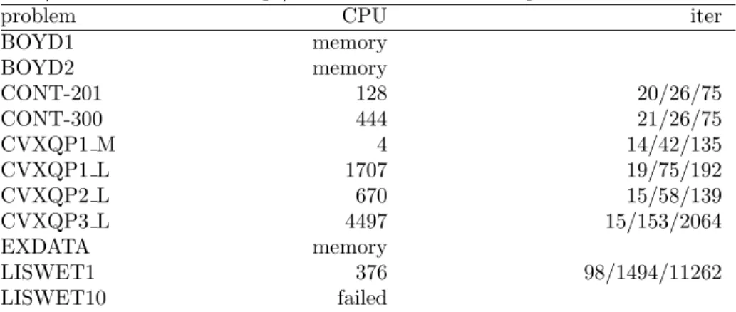
The next Table 2 gives CPU times and iteration counts for selected examples (following [13]).
Table 2: Computational results for selected QP problems using PENNON, performed on Pentium III-M (1000 MHz) with 512 KB memory running SuSE LINUX 7.3. The values in column “iter” denote number of outer itera-tions/number of Newton steps/number of line-search steps.
problem CPU iter
BOYD1 memory BOYD2 memory CONT-201 128 20/26/75 CONT-300 444 21/26/75 CVXQP1 M 4 14/42/135 CVXQP1 L 1707 19/75/192 CVXQP2 L 670 15/58/139 CVXQP3 L 4497 15/153/2064 EXDATA memory LISWET1 376 98/1494/11262 LISWET10 failed
6.2
mater
problems
Program PENNON, both the NLP and SDP versions, was actually developed as a part of a software package MOPED for material optimization. The goal of this
package is to design optimal structures considered as two- or three-dimensional continuum elastic bodies where the design variables are thematerial properties which may vary from point to point. Our aim is to optimize not only the distribution of material but also the material properties themselves. We are thus looking for the ultimately best structure among all possible elastic continua, in a framework of what is now usually referred to as “free material design” (see [21] for details). After analytic reformulation and discretization by the finite element method, the problem reduces to a large-scale convex NLP problem
min
α∈R,x∈RN
α−cTx|α≥xTAixfori= 1, . . . , M
with positive semidefinite matricesAi. HereM is the number of finite elements
and N the number of degrees of freedom of the displacement vector. For real world problems one should work with discretizations of sizeM ≈20 000.
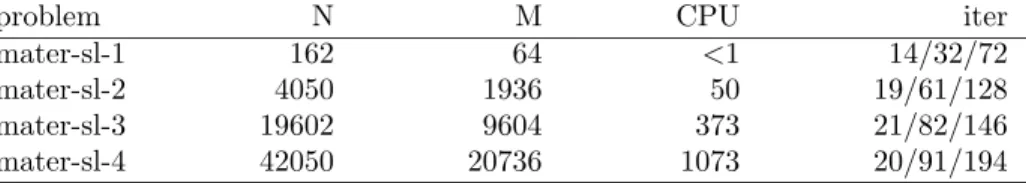
For the purpose of this paper we used an AMPL model of a typical material optimization problem. The examples presented in Table 3 differ in the number of variables and constraints but their character is the same. We must remark that a direct implementation of the problem (without the AMPL interface) leads to much more efficient solution, in terms of memory and CPU time.
Table 3: Computational results for mater problems using PENNON, performed on Pentium III-M (1000 MHz) with 512 KB memory running SuSE LINUX 7.3. “N” is the number of variables “M” the number of constraints. The values in col-umn “iter” denote number of outer iterations/number of Newton steps/number of line-search steps.
problem N M CPU iter
mater-sl-1 162 64 <1 14/32/72
mater-sl-2 4050 1936 50 19/61/128
mater-sl-3 19602 9604 373 21/82/146
mater-sl-4 42050 20736 1073 20/91/194
6.3
SDPLIB
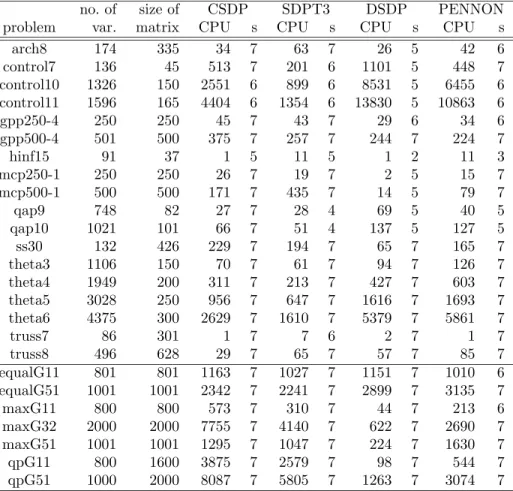
Due to space limitations, we do not present here the full SDPLIB results and select just several representative problems. Table 4 lists the selected SDPLIB problems, along with their dimensions, and the results for CSDP, SDPT3, DSDP, and PENNON2. All codes were used with standard setting; CSDP and
PENNON were linked with ATLAS-BLAS library, SDPT3 (with HKM direc-tion) ran under Matlab 6.1.
In several SDPLIB problems, CSDP, SDPT3 or DSDP are faster than PEN-NON. This is, basically, due to the number of Newton steps used by the par-ticular algorithms. Since the complexity of Hessian assembling is about the same for all three codes, and the data sparsity is handled in a similar way, the main time difference is given by the number of Newton steps. While CSDP and SDPT3 need, in average, 15–30 steps, PENNON needs about 2–3 times more steps. Recall that this is due to the fact that PENNON is based on an
2
This table is overtaken fromftp://plato.la.asu.edu/pub/sdplib.txtwith a kind per-mission of the author.
Table 4: Selected SDPLIB problems and computational results using CSDP, SDPT3, and PENNON, performed on a Pentium II PC (450 MHz) with 512 KB memory running LINUX-2.4.14 and Matlab 6.1. “s” is the number of correct digits in the objective function.
no. of size of CSDP SDPT3 DSDP PENNON
problem var. matrix CPU s CPU s CPU s CPU s
arch8 174 335 34 7 63 7 26 5 42 6 control7 136 45 513 7 201 6 1101 5 448 7 control10 1326 150 2551 6 899 6 8531 5 6455 6 control11 1596 165 4404 6 1354 6 13830 5 10863 6 gpp250-4 250 250 45 7 43 7 29 6 34 6 gpp500-4 501 500 375 7 257 7 244 7 224 7 hinf15 91 37 1 5 11 5 1 2 11 3 mcp250-1 250 250 26 7 19 7 2 5 15 7 mcp500-1 500 500 171 7 435 7 14 5 79 7 qap9 748 82 27 7 28 4 69 5 40 5 qap10 1021 101 66 7 51 4 137 5 127 5 ss30 132 426 229 7 194 7 65 7 165 7 theta3 1106 150 70 7 61 7 94 7 126 7 theta4 1949 200 311 7 213 7 427 7 603 7 theta5 3028 250 956 7 647 7 1616 7 1693 7 theta6 4375 300 2629 7 1610 7 5379 7 5861 7 truss7 86 301 1 7 7 6 2 7 1 7 truss8 496 628 29 7 65 7 57 7 85 7 equalG11 801 801 1163 7 1027 7 1151 7 1010 6 equalG51 1001 1001 2342 7 2241 7 2899 7 3135 7 maxG11 800 800 573 7 310 7 44 7 213 6 maxG32 2000 2000 7755 7 4140 7 622 7 2690 7 maxG51 1001 1001 1295 7 1047 7 224 7 1630 7 qpG11 800 1600 3875 7 2579 7 98 7 544 7 qpG51 1000 2000 8087 7 5805 7 1263 7 3074 7
algorithm for general nonlinear convex problems and allows to solve larger class of problems. This is the price we pay for the generality. We believe that, in this light, the code is competitive.
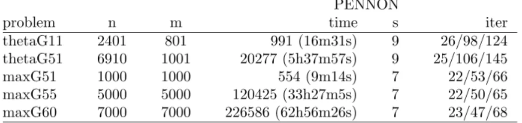
The SDPLIB collection includes some very-large-scale problems, which are impossible to solve on a PC, due to memory limitations. We have solved these problems on an SGI Origin 3400 parallel computer with 56 GB main memory. We did not use any paralellization of PENNON but linked it with parallel BLAS and LAPACK libraries. The examples were solved using 4 processors. Table 5 shows the computational time needed by PENNON. We did not compare these times with any other SDP code; the purpose of these tests was to see whether PENNON is able to solve these large-scale problems and whether its behaviour deteriorates in any way. The results show that PENNON is very robust, at least for this group of problems. (To get a comparison with other computers, we included a smaller problem maxG51, contained in Table 4 above. Obviously, such comparison of a sequential and parallel computer gives only a very vague idea.).
Table 5: Computational results on large SDPLIB problems using PENNON, performed on SGI Origin 3400 with 56 GB memory using 4 processors. The values in column “iter” denote number of outer iterations/number of Newton steps/number of line-search steps. “s” is the number of correct digits in the objective function.
PENNON
problem n m time s iter
thetaG11 2401 801 991 (16m31s) 9 26/98/124
thetaG51 6910 1001 20277 (5h37m57s) 9 25/106/145
maxG51 1000 1000 554 (9m14s) 7 22/53/66
maxG55 5000 5000 120425 (33h27m5s) 7 22/50/65
maxG60 7000 7000 226586 (62h56m26s) 7 23/47/68
6.4
mater
and
truss
problems
Next we present results of two sets of examples coming from structural optimiza-tion. The first set contains examples from free material optimization introduced above. While the single-load problem can be formulated as a convex NLP, the more realistic multiple-load is modeled by linear SDP as described in [1]. All examples solve the same problem (geometry, loads, boundary conditions) and differ only in the finite element discretization.
The linear matrix operatorA(x) =PAixi has the following structure: Ai
are block diagonal matrices with many (∼5 000) small (11×11–20×20) blocks. Moreover, only few (6–12) of these blocks are nonzero in anyAi, as schematically
shown in the figure below.
2
x +
1x + ...
As a result, the Hessian of the augmented Lagrangian associated with this prob-lem is a large and sparse matrix. PENNON proved to be particularly efficient for this kind of problems, as shown in Table 7.
The following results are overtaken from Mittelmann [13] and were obtained3
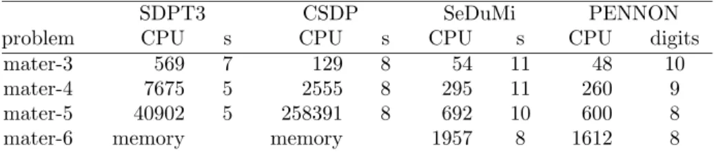
on Sun Ultra 60, 450 MHz with 2 GB memory, running Solaris 8. Table 6 shows the dimensions of the problems, together with the optimal objective value. Ta-ble 7 presents the test results for CSDP, SDPT3 and PENNON. It turned out that for this kind of problems, the code SeDuMi by Sturm [17] was rather com-petitive, so we included also this code in the table.
In the second set, we solve problems from truss topology design:
• trtoare problems from single-load truss topology design. Normally for-mulated as LP, here reforfor-mulated as SDP for testing purposes (see, eg, [2, 11]).
3
Except of mater-5 solved by CSDP and mater-6 solved by CSDP and SDPT3. These were obtained using Sun E6500, 400 MHz with 24 GB memory
Table 6: materproblems
problem n m Optimal value
mater-3 1439 3588 -1.339163e+02
mater-4 4807 12498 -1.342627e+02
mater-5 10143 26820 -1.338016e+02
mater-6 20463 56311 -1.335387e+02
Table 7: Computational results for mater problems using SDPT3, CSDP, Se-DuMi, and PENNON, performed on a Sun Ultra 60 (450 MHz) with 2 GB of memory running Solaris 8. “s” is the number of correct digits in the objective function.
SDPT3 CSDP SeDuMi PENNON
problem CPU s CPU s CPU s CPU digits
mater-3 569 7 129 8 54 11 48 10
mater-4 7675 5 2555 8 295 11 260 9
mater-5 40902 5 258391 8 692 10 600 8
mater-6 memory memory 1957 8 1612 8
• vibraare single load truss topology problems with a vibration constraint. The constraint guarantees that the minimal self-vibration frequency of the optimal structure is bigger than a given value; see [9].
• buckare single load truss topology problems with linearized global buck-ling constraint. Originally a nonlinear matrix inequality, the constraint should guarantee that the optimal structure is mechanically stable (does not buckle); see [9].
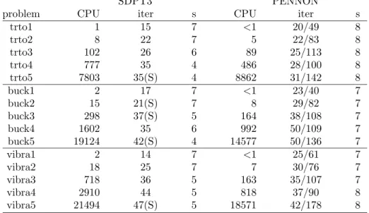
All problems from this set are characterized by sparsity of the linear matrix operator A. These problems are very difficult to solve. From all the tested SDP solvers, only SDPT3 and PENNON, followed by DSDP, could solve them efficiently. SeDuMi could only solve small problems and needed unacceptable length of time for larger ones. CSDP crashed on almost all problems from this set. In the following tables, we only show comparison of PENNON with SDPT3. Table 8 gives problem characteristics, while Table 9 presents results of the test runs.
When we started to test these examples with PENNON, we realized that the line-search procedure is very inefficient for this group of problems. It turned out that it is much more efficient to avoid line-search and do always a full Newton step. Results in Table 9 were obtained with this version of the code. This idea (to avoid line-search) is, however, not always a good one (in some SDPLIB examples), and this part of the algorithm needs certainly more attention and future development.
6.5
DIMACS
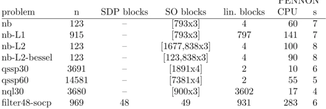
Finally, in Table 10 we present results of selected problems from the DIMACS collection. These are mainly SOCP problems, apart from filter48-socpthat combines SOCP and SDP constraints. The results demonstrate that we can reach high accuracy even when working with the smooth reformulation of the
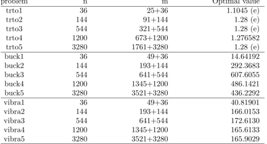
Table 8: truss problems. (e) denotes known exact optimal value; n is the number of variables,mthe size of the matrix constraint; 25+36 means: matrix constraint of size 25 and 36 linear constraints
problem n m Optimal value
trto1 36 25+36 1.1045 (e) trto2 144 91+144 1.28 (e) trto3 544 321+544 1.28 (e) trto4 1200 673+1200 1.276582 trto5 3280 1761+3280 1.28 (e) buck1 36 49+36 14.64192 buck2 144 193+144 292.3683 buck3 544 641+544 607.6055 buck4 1200 1345+1200 486.1421 buck5 3280 3521+3280 436.2292 vibra1 36 49+36 40.81901 vibra2 144 193+144 166.0153 vibra3 544 641+544 172.6130 vibra4 1200 1345+1200 165.6133 vibra5 3280 3521+3280 165.9029
SOCP constraints (see Section 5.1). The results also show the influence of linear constraints on the efficiency of the algorithm; cf. problemsnbandnb-L1. This is due to the fact that, in our algorithm, the part of the Hessian corresponding to every (penalized) linear constraint is a dyadic, i.e., possibly full matrix. We are working on an approach that treats linear constraints separately.
Acknowledgment
The authors would like to thank Hans Mittelmann for his help when testing the code and for implementing PENNON on the NEOS server. This research was supported by BMBF project 03ZOM3ER. The first author was partly supported by grant No. 201/00/0080 of the Grant Agency of the Czech Republic.
References
[1] A. Ben-Tal, M. Koˇcvara, A. Nemirovski, and J. Zowe. Free material design via semidefinite programming. The multi-load case with contact conditions. SIAM J. Optimization, 9:813–832, 1997.
[2] A. Ben-Tal and A. Nemirovski. Lectures on Modern Convex Optimization. MPS-SIAM Series on Optimization. SIAM Philadelphia, 2001.
[3] A. Ben-Tal and M. Zibulevsky. Penalty/barrier multiplier methods for convex programming problems. SIAM J. Optimization, 7:347–366, 1997. [4] S. J. Benson and Y. Ye. DSDP4 users manual. Report
ANL/MCS-TM-248, Argonne National Laboratory, Argonne, 2002. Available at http://www-unix.mcs.anl.gov/~benson/.
Table 9: Computational results for truss problems using SDPT3 and PEN-NON, performed on a Pentium III PC (650 MHz) with 512 KB memory running SuSE LINUX 7.3. (S) means that the code failed with “Schur complement not positive definite” or “Lack of progress” but close to convergence, usually 5–6 dig-its accuracy. For PENNON, “iter” denotes number of outer iterations/number of Newtons steps. “s” is the number of correct digits in the objective function.
SDPT3 PENNON
problem CPU iter s CPU iter s
trto1 1 15 7 <1 20/49 8 trto2 8 22 7 5 22/83 8 trto3 102 26 6 89 25/113 8 trto4 777 35 4 486 28/100 8 trto5 7803 35(S) 4 8862 31/142 8 buck1 2 17 7 <1 23/40 7 buck2 15 21(S) 7 8 29/82 7 buck3 298 37(S) 5 164 38/108 7 buck4 1602 35 6 992 50/109 7 buck5 19124 42(S) 4 14577 50/136 7 vibra1 2 14 7 <1 25/61 7 vibra2 18 25 7 7 30/76 7 vibra3 718 36 5 163 35/107 7 vibra4 2910 44 5 818 37/90 8 vibra5 21494 47(S) 5 18571 42/178 8
[5] B. Borchers. CSDP, a C library for semidefinite programming. Op-timization Methods and Software, 11:613–623, 1999. Available at http://www.nmt.edu/~borchers/.
[6] B. Borchers. SDPLIB 1.2, a library of semidefinite programming test prob-lems. Optimization Methods and Software, 11 & 12:683–690, 1999. Avail-able athttp://www.nmt.edu/~borchers/.
[7] R. Fourer, D. M. Gay, and B. W. Kerningham. AMPL: A Modeling Lan-guage for Mathematical Programming. The Scientific Press, 1993.
[8] K. Fujisawa, M. Kojima, and K. Nakata. Exploiting sparsity in primal-dual interior-point method for semidefinite programming. Mathematical Programming, 79:235–253, 1997.
[9] M. Koˇcvara. On the modelling and solving of the truss design problem with global stability constraints. Struct. Multidisc. Optimization, 2002. In print.
[10] M. Koˇcvara and M. Stingl. PENNON—a generalized augmented La-grangian method for semidefinite programming. Preprint 286, Institute of Applied Mathematics, University of Erlangen, 2001.
[11] M. Koˇcvara and J. Zowe. How mathematics can help in design of mechanical structures. In D.F. Griffiths and G.A. Watson, editors,Numerical Analysis 1995, pages 76–93. Longman, Harlow, 1996.
Table 10: Computational results on DIMACS problems using PENNON, per-formed on a Pentium III PC (650 MHz) with 512 KB memory running SuSE LINUX 7.3. Notation like [793x3] indicates that there were 793 (semidefinite, second-order, linear) blocks, each a symetric matrix of order 3.
PENNON
problem n SDP blocks SO blocks lin. blocks CPU s
nb 123 – [793x3] 4 60 7 nb-L1 915 – [793x3] 797 141 7 nb-L2 123 – [1677,838x3] 4 100 8 nb-L2-bessel 123 – [123,838x3] 4 90 8 qssp30 3691 – [1891x4] 2 10 6 qssp60 14581 – [7381x4] 2 55 5 nql30 3680 – [900x3] 3602 17 4 filter48-socp 969 48 49 931 283 6
[12] I. Maros and C. M´esz´aros. A repository of convex quadratic programming problems. Optimization Methods and Software, 11&12:671–681, 1999. [13] H. Mittelmann. Benchmarks for optimization software. Available at
http://plato.la.asu.edu/bench.html.
[14] L. Mosheyev and M. Zibulevsky. Penalty/barrier multiplier algorithm for semidefinite programming. Optimization Methods and Software, 13:235– 261, 2000.
[15] E. Ng and B. W. Peyton. Block sparse cholesky algorithms on advanced uniprocessor computers. SIAM J. Scientific Computing, 14:1034–1056, 1993.
[16] G. Pataki and S. Schieta. The DIMACS library of mixed semidefinite-quadratic-linear problems. Available at http://dimacs.rutgers.edu/challenges/seventh/instances.
[17] J. Sturm. Using SeDuMi 1.02, a MATLAB toolbox for optimization over symmetric cones. Optimization Methods and Software, 11 & 12:625–653, 1999. Available athttp://fewcal.kub.nl/sturm/.
[18] R.H. T¨ut¨unc¨u, K.C. Toh, and M.J. Todd. SDPT3 — A MATLAB software package for semidefinite-quadratic-linear programming, Version 3.0. Avail-able athttp://www.orie.cornell.edu/~miketodd/todd.html, School of Operations Research and Industrial Engineering, Cornell University, 2001. [19] M. Zibulevsky. New penalty/barrier and lagrange multiplier approach for semidefinite programming. Research Report 5/95, Optimization Labora-tory, Technion, Israel, 1995.
[20] M. Zibulevsky.Penalty/barrier multiplier methods for large-scale nonlinear and semidefinite programming. PhD thesis, Technion—Israel Institute of Technology, Haifa, 1996.
[21] J. Zowe, M. Koˇcvara, and M. Bendsøe. Free material optimization via mathematical programming.Mathematical Programming, Series B, 79:445– 466, 1997.