Testing effort dependent software reliability model for imperfect debugging process considering both detection and correction

(1)

http://wrap.warwick.ac.uk

Original citation:

Peng, R., Li, Y. F., Zhang, Wenjuan and Hu, Q. P.. (2014) Testing effort dependent

software reliability model for imperfect debugging process considering both detection

and correction. Reliability Engineering & System Safety, Volume 126 . pp. 37-43. ISSN

0951-8320

Permanent WRAP url:

http://wrap.warwick.ac.uk/59044

Copyright and reuse:

The Warwick Research Archive Portal (WRAP) makes this work of researchers of the

University of Warwick available open access under the following conditions.

This article is made available under the Creative Commons Attribution 3.0 (CC BY 3.0)

license and may be reused according to the conditions of the license. For more details

see:

http://creativecommons.org/licenses/by/3.0/

A note on versions:

The version presented in WRAP is the published version, or, version of record, and may

be cited as it appears here.

(2)

Testing effort dependent software reliability model for imperfect

debugging process considering both detection and correction

$

R. Peng

a,n

, Y.F. Li

b

, W.J. Zhang

c

, Q.P. Hu

d

a

Dongling School of Economics & Management, University of Science & Technology Beijing, China b_{Ecole Centrale Paris-SUPELEC, Paris, France}

c

Warwick Business School, The University of Warwick, Coventry CV4 7AL, UK d

Academy of Mathematics and Systems Science, Chinese Academy of Sciences, Beijing, China

a r t i c l e i n f o

Article history:

Received 2 May 2012 Received in revised form 3 January 2014 Accepted 5 January 2014 Available online 11 January 2014

Keywords:

Software reliability Fault detection process Fault correction process Testing effort function Imperfect debugging

a b s t r a c t

This paper studies the fault detection process (FDP) and fault correction process (FCP) with the incorporation of testing effort function and imperfect debugging. In order to ensure high reliability, it is essential for software to undergo a testing phase, during which faults can be detected and corrected by debuggers. The testing resource allocation during this phase, which is usually depicted by the testing effort function, considerably influences not only the fault detection rate but also the time to correct a detected fault. In addition, testing is usually far from perfect such that new faults may be introduced. In this paper, wefirst show how to incorporate testing effort function and fault introduction into FDP and then develop FCP as delayed FDP with a correction effort. Various specific paired FDP and FCP models are obtained based on different assumptions of fault introduction and correction effort. An illustrative example is presented. The optimal release policy under different criteria is also discussed.

1. Introduction

As software is becoming more and more widely used, both the functionality and the correctness of software are of great concern. In order to ensure high reliability, testing is usually conducted, during which faults in software manifest by causing failures and can be detected and removed by debuggers[9,4,15]. On the other hand, it is almost impossible to make bug-free software even though scientiﬁc and disciplined development practices are fol-lowed. During the last 30 years, many software reliability growth models (SRGMs) have been proposed as a tool to track the reliability growth trend of the software testing process

[16,3,35,23]. SRGMs are very useful in the sense that they can help management making critical decisions, such as testing resource allocation and the determination of software release time[19,13,12].

Testing consumes a large amount of resources, such as man-power and CPU hours, which are usually not constantly allocated during testing phase. The function that describes how testing resources are distributed is usually referred to as testing effort function (TEF) and it has been incorporated into software

reliability studies by some researchers [30,16,17]. Yamada et al.

[34]pointed out that the TEF could be described by a Weibull-type distribution, which actually includes Exponential curve, Rayleigh curve and Weibull curve. Weibull-type curve can wellﬁt most data and is often used in theﬁeld of software reliability modeling[7]. Logistic TEF is used instead of Weibull-type TEF by some research-ers and appeared to be fairly accurate in describing the consump-tion of testing effort[24,5,8].

Generally a detected fault cannot be corrected immediately and the time required to correct a detected fault is usually called debugging lag/delay. The idea of modeling the fault correction process (FCP) wasﬁrst proposed in Schneidewind[28], in which it was modeled as a separate process following the fault detection process (FDP) with a constant time lag. Based on this framework, Xie et al.[33]and Wu et al.[31]proposed several paired FDP and FCP models through incorporating other variants of debugging delay. Later, Hwang and Pham[10]developed a generalized NHPP model considering quasi-renewal time-delay fault removal. Jia et al. [14] proposed a Markovian software reliability model considering the fault correction process. However, the inﬂuence of testing effort on debugging lag is not considered in these papers. Intuitively, the time needed to correct a detected fault, or the debugging lag, tends to be shorter if more testing effort is allocated during the period between detection and correction of the fault. Thus it is more reasonable to incorporate testing effort function into the modeling framework on both FDP and FCP.

Contents lists available atScienceDirect

journal homepage:www.elsevier.com/locate/ress

Reliability Engineering and System Safety

http://dx.doi.org/10.1016/j.ress.2014.01.004

☆_{This is an open-access article distributed under the terms of the Creative}

Commons Attribution License, which permits unrestricted use, distribution, and reproduction in any medium, provided the original author and source are credited.

n_{Corresponding author. Tel.:}_þ_{86 13051540519.} E-mail address:[email protected](R. Peng).

(3)

Moreover, the debugging process is usually far from perfect and actually many faults encountered by customers are those intro-duced during debugging[36,29,6,26]. It is essential to incorporate imperfect debugging into FDP and FCP models[32,2,18].

In this paper, a framework is proposed to develop testing effort dependent FDP and FCP models with the consideration of imperfect debugging. The rest of this paper is organized as follows. InSection 2, a framework is proposed to obtain testing effort dependent paired FDP and FCP models with the considera-tion of fault introducconsidera-tion. In Section 3, several speci_ﬁc models are derived based on different assumptions of fault introduction and the correction effort. In Section 4, several commonly used testing effort functions are reviewed. InSection 5, an illustrative example is presented. The optimal release policy under different criteria is studied inSection 6. Conclusions and discussions are presented inSection 7.

2. Testing effort dependent FDP and FCP models with fault introduction

The expected total number of faults at timetis denoted by the fault content rate functiona(t), which is the sum of the number of initial faults in the software a(¼a(0)) and the number of faults introduced during time interval [0,t). We usew(t) to denote the time dependent testing effort rate and W(t) to denote the cumulative testing effort consumed till timet.

2.1. FDP model

Mean value function md(t) is used to depict the expected number of faults detected till timetandλdðtÞ ¼dmdðtÞ=dtis used to denote the fault intensity function. The number of faults detected during time interval [t,tþΔt) by current testing effort expenditure is usually assumed to be proportional to the number of remaining faults at timet[21]. Hence we have

λdðtÞ ¼dmdðtÞ

dt ¼bðtÞwðtÞðaðtÞmdðtÞÞ ð1Þ whereb(t) is the current fault detection rate per unit of testing effort at timet, andw(t) is the current testing effort expenditure at timet. Substituting the marginal conditionmd(0)¼0 into (1) gives mdðtÞ ¼aðtÞaexp Z t 0 bðxÞwðxÞdx exp Z t 0 bðxÞwðxÞdx Z t 0 a0ðxÞexpf Z x 0 bðyÞwðyÞdy dx ð2Þ where a0ðxÞ ¼daðxÞ=dx. Various md(t) can be derived based on different assumptions ofa(t),b(t) andw(t).λdðtÞcan be obtained by substituting (2) into the right hand side of (1) as

λdðtÞ ¼dmdðtÞ dt ¼abðtÞwðtÞexp Z t 0 bðxÞwðxÞdx 1þZ t 0 a0ðxÞ a exp Z x 0 bðyÞwðyÞdy dx ð3Þ 2.2. FCP model

Mean value function mr(t) is used to denote the expected number of faults removed till timetandλrðtÞ ¼dmrðtÞ=dtis used

to denote the fault removal intensity function. Since a removed fault must ﬁrst be detected, FCP can be modeled as a separate process following FDP with a debugging delay. For convenience of discussion, the testing effort consumed during the period from detection of a fault to theﬁnal removal of the fault is termed as correction effort of the fault. Generally correcting different faults requires different amounts of testing resources, hence correction effort can be modeled as a random variable with probability density function (pdf) and the cumulative distribution function (cdf) denoted asf(x) andF(x).

Thus it can be obtained that mrðtÞ ¼

Z t

0 λd

ðyÞFðWðtÞWðyÞÞdy ð4Þ whereFðWðtÞWðyÞÞis the probability that the fault detected aty is corrected beforet.

Differentmr(t) can be derived based onmd(t) and differentf(x). Furthermore, we have λrðtÞ ¼Z t 0 λd ðyÞfðWðtÞWðyÞÞwðtÞdy ¼Z Wn ðtÞ 0 λd ðW1ðWðtÞxÞÞfðxÞwðtÞdðW1ðWðtÞxÞÞ ¼Z WnðtÞ 0 λd ðW1ðWðtÞxÞÞfðxÞwðtÞ dx wðW1ðWðtÞxÞÞ ð5Þ Differentmr(t) can be derived based onmd(t) and differentf(x).

3. Some speciﬁc models

Fault detection rate function b(t) is usually assumed to be constant and it is denoted asbhere[21]. From (2) we have mdðtÞ ¼aðtÞaexpfbWnðtÞgexpfbWnðtÞg

Zt 0

a0ðxÞexpfbWn_ðxÞgdx

ð6Þ The total number of faultsa(t) was usually assumed to be an expo-nential or linear function of time in the literature. Yamada et al.[34]

proposed two FDP models with consideration of imperfect debugging, by assuming that the expected total number of faults increases exponentially and linearly with the testing time, respectively. An S-shaped concave FDP model was proposed in Pham et al.[25]

assuming that the total number of faults is a linear function of the testing time. In the following subsections various TEF dependent FDP and FCP models are derived based on different assumptions ona(t) andf(x).

3.1. Paired model 1

We assume that the total number of faults increases exponen-tially with the total testing effort consumed and the correction effort required is an exponential variable as

aðtÞ ¼aexpfαWnðtÞg; αZ0 ð7Þ

fðxÞ ¼cexpfcxg ð8Þ

In this case we have mdðtÞ ¼ ab bþαðexp αWnðtÞ expbWnðtÞÞ ð9Þ mrðtÞ ¼ ab ðbþαÞ2ðbexpfαWnðtÞgþαexpfbWnðtÞgÞ ab ðbþαÞð1þbWnðtÞÞexpfbWnðtÞg; c¼b a ð1þα=bÞ cexpfαWn_ð_t_{Þg þ}_α_expf_cWn_ð_t_Þg cþα þ cexpf bWn_ð_t_Þg_b_expf_cWn_ð_t_Þg bc ; cab 8 > < > : ð10Þ

R. Peng et al. / Reliability Engineering and System Safety 126 (2014) 37–43

(4)

Actually (9) can be obtained by combining (6) and (7). (10) can be obtained by substituting (9) into (3), and (4). WhenWn(t)¼t, (9) is the same as the FDP model obtained in Yamada et al.[34]for the case when the total number of faults is an exponential function of testing time. Whenα¼0 andWn(t)¼t, (9) and (10) are the same as the paired model obtained in Wu et al.[31] for the case of exponential debugging delay.

3.2. Paired model 2

We assume that the total number of faults increases exponen-tially with the total testing effort consumed as given in (7) and the correction effort required is a gamma variable as

fðxÞ ¼μexpfμxgðμxÞc1

ΓðcÞ ; c; m40 ð11Þ

whereΓðcÞ ¼R₀1expfygyc1_dy_{is the Euler gamma function.} Similarly we have mdðtÞ ¼ ab bþαðexp αWnðtÞ expbWnðtÞÞ ð12Þ mrðtÞ ¼ aexpfαWnðtÞgΓðc;0;ðbþαÞWn_ðtÞÞ 1þα b ð Þcþ1 ΓðcÞ aΓðc;0;bWnðtÞÞ 1þα b ð ÞΓðcÞ þaΓ ðcþ1;0;bWnðtÞÞ 1þα b ð ÞcΓðcÞ Þ; μ¼b aexpfαWn_ðtÞg_Γ_ðc_;₀_;_ð_μ_þ_α_ÞWn_ðtÞÞ 1þα b ð Þ1þα μ c ΓðcÞ aexpf bWn_ðtÞg_Γ_ðc_;₀_;_ð_μ_bÞWn_ðtÞÞ 1þα b ð Þ1b μ c ΓðcÞ ; μab 8 > > < > > : ð13Þ where _Γðε1;ε2;ε3Þ ¼R_εε3 2e y_yε11_dy _{is a generalized incomplete}

gamma function. Whenα¼0 and Wn(t)¼t, (12) and (13) are the same as the paired model obtained in Wu et al.[31]for the case of gamma debugging delay.

3.3. Paired model 3

We assume that the total number of faults increases linearly with the total testing effort consumed and the correction effort required is an exponential variable as

aðtÞ ¼aþsWnðtÞ; sZ0 ð14Þ

fðxÞ ¼cexpfcxg ð15Þ

In this case we have mdðtÞ ¼ a

s b

ð1expbWnðtÞÞþsWnðtÞ ð16Þ

Actually (16) can be obtained by combining (6) and (14). (17) can be obtained by substituting (16) into (3) and (4). WhenWn(t)¼t, (16) is the same as the FDP model obtained in Yamada et al.[34]for the case when the total number of faults is a linear function of testing time. When s¼0 and Wn(t)¼t, (16) and (17) are the same as the paired model obtained in Wu et al.[31]for the case of exponential debugging delay.

3.4. Paired model 4

We assume that the total number of faults increases linearly with the total testing effort consumed as given in (14) and the correction effort required is a gamma variable as given in (11).

Similarly we have mdðtÞ ¼ a s b ð1expbWnðtÞÞþsWnðtÞ ð18Þ mrðtÞ ¼ swðtÞ bΓðcÞðbWnðtÞΓðc;0;bWnðtÞΓðcþ1;0;bWnðtÞÞþðas=bÞcΓðcÞ Γðcþ1;0;bWnðtÞÞ;μ¼b s μΓðcÞðμWnðtÞΓðc;0;μWnðtÞΓðcþ1;0;μWnðtÞÞ þðas=bÞ ΓðcÞ Γðc;0;μWnðtÞÞðas=bÞexpf bW nðtÞg ΓðcÞð1b=μÞc Γðc;0;ðμbÞWnðtÞÞ; cab 8 > > > > < > > > > : ð19Þ whens¼0 andWn(t)¼t, (18) and (19) are the same as the paired model obtained in Wu et al. [31] for the case of gamma debugging delay.

4. A summary of various testing effort functions

Testing effort functions that have been commonly used include Constant, Exponential, Rayleigh, Weibull and Logistic curves. Exponential curve and Rayleigh curve can be regarded as special cases of Weibull curve. The details are shown below.

4.1. Constant TEF

We assume thatw(t) is a constant. It can be expressed as

wðtÞ ¼w ð20Þ

Thus the cumulative testing effortW(t) can be obtained as

WðtÞ ¼wt ð21Þ

It can be seen that the total testing effort consumed tends to positive in_ﬁnity, whentapproaches positive in_ﬁnity. In the case that TEF is not considered, it can be regarded as consideringw(t)¼1.

4.2. Weibull TEF

Weibull TEF is veryﬂexible and it can wellﬁt most data that are often used in the study of SRGM. The cumulative TEFW(t) is given by

WðtÞ ¼Nð1expfβtmgÞ ð22Þ

whereNis the expected total amount of testing effort that is required by software testing. β and m are the scale parameter and shape parameter, respectively. It should also be noted that the cumulative testing effort consumed isﬁnite and tends toNwhentapproaches positive inﬁnity.

Differentiating (22) gives wðtÞ ¼Nβmtm1

expfβtm_g _ð₂₃_Þ

The exponential TEF is a special case of Weibull TEF whenm¼1. Exponential curve is suitable to describe the testing environment which has a monotonically declining testing effort rate.

The Rayleigh TEF is a special case of Weibull TEF when m¼2. Rayleigh testing effort rateﬁrst increases to its peak, then decreases with a decelerating speed to zero asymptotically without reaching zero. mrðtÞ ¼ a2s b _ð 1ð1þbWnðtÞÞexpbWnðtÞþsWnðtÞð1expbWnðtÞÞ; c¼b as b 1þbexpf cWnðtÞg cexpf bWnðtÞg cb þsWnðtÞs cð1exp ( cWnðtÞ gÞ;cab 8 > > < > > : ð17Þ

(5)

4.3. Logistic TEF

Logistic curve wasﬁrst proposed in Parr[24]as an alternative of Rayleigh curve. It exhibits similar behavior as Rayleigh curve, except during the initial stage of the project. The logistic cumu-lative TEFW(t) is given by

WðtÞ ¼ N

1þAexpfηtg ð24Þ

whereAis a constant parameter andηis the consumption rate of testing effort expenditure. Similar to the Weibull case, the cumu-lative testing effort consumed is _ﬁnite and tends to N when t approaches positive inﬁnity.

Taking derivatives on both sides of (24) gives wðtÞ ¼ NAη exp η2t þAexp η t 2 2 ð25Þ

w(t) reaches its maximum value whent¼lnA₌_η.

5. Illustrative example

5.1. Dataset description

The dataset we use is from the System T1 data of the Rome Air Development Center (RADC) [22]. Although this is quite an old dataset, it is widely used and it contains both fault detection data and fault correction data. Additionally, it contains information of testing effort, which is characterized by computer time (CPU hours) consumed in each week. Hence this familiar dataset is used for illustration.

The cumulative numbers of detected faults and corrected faults during theﬁrst 21 weeks are shown inTable 1. During the time span, totally 300.1 CPU hours were consumed. Till the end of the testing, 136 faults were detected and all of them were corrected.

5.2. Select the most suitable TEF for this dataset

Parameters in the different types of TEF are estimated by Least Square Error (LSE). In order to select a TEF that best ﬁts this

dataset, some criteria are used to compare the performances of different TEFs.

(1) RMSE

The Root Mean Square Error (RMSE) is defined as RMSE¼ ffiffiffiffiffiffiffiffiffiffiffiffiffiffiffiffiffiffiffiffiffiffiffiffiffiffiffiffiffiffiffiffiffiffiffiffiffiffi 1 n ∑ n i¼1 ðwðtiÞwiÞ2 s ð26Þ A smaller RMSE indicates a smaller fitting error and better performance.

(2) Bias

The bias is deﬁned as the sum of the deviation of the estimated testing curve from the actual data, as shown below:

Bias¼1 n ∑ n i¼1 ðwðtiÞwiÞ ð27Þ (3) Variance

The variance is defined as[8] Variance¼ ffiffiffiffiffiffiffiffiffiffiffiffiffiffiffiffiffiffiffiffiffiffiffiffiffiffiffiffiffiffiffiffiffiffiffiffiffiffiffiffiffiffiffiffiffiffiffiffiffiffiffi 1 n ∑ n i¼1 ðwðtiÞwiBiasÞ2 s ð28Þ (4) RMSPE

The Root Mean Square Prediction Error (RMSPE) is defined as[8] RMSPE¼pffiffiffiffiffiffiffiffiffiffiffiffiffiffiffiffiffiffiffiffiffiffiffiffiffiffiffiffiffiffiffiffiffiffiffiVarianceþBias2 _ð₂₉_Þ RMSPE is also a measure to depict how close the model predicts the observation.

Estimated parameters and comparison results for different TEFs are shown inTable 2.Fig. 1is plotted for graphical illustration.

It can be seen that logistic TEF has the smallest RMSE, Variance, and RMSPE and also has a smaller Bias than Weibull TEF.Fig. 1also shows that logistic TEFﬁts best. Thus logistic TEF is adopted for further analysis.

5.3. Performance analysis

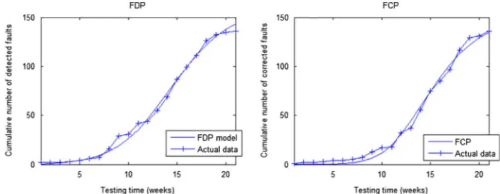
The paired model (9) and (10) is used for illustration. After substituting the cumulative logistic testing effort function (24) with the estimated parameters N¼321.482, η¼0.3826, and A¼423.788 into (9) and (10), the paired model is applied to ﬁt against the real dataset. The LSE estimation of the parameters are obtained as a¼100.97, b¼0.0094, α¼0.0021 and c¼0.0418. According to the estimated parameters, there are about 100.97 faults at the beginning of testing. The total number of faults whent approaches inﬁnity is expected to be limt-1aðtÞ ¼198:01.Fig. 2is plotted for graphical illustration.

Table 1

The dataset–System T1. Weeks Computer time (CPU hours) Cumulative number of detected faults Cumulative number of corrected faults 1 4 2 1 2 4.3 2 2 3 2 2 2 4 0.6 3 3 5 2.3 4 4 6 1.6 6 4 7 1.8 7 5 8 14.7 16 7 9 25.1 29 13 10 4.5 31 17 11 9.5 42 18 12 8.5 44 32 13 29.5 55 37 14 22 69 56 15 39.5 87 75 16 26 99 85 17 25 111 97 18 31.4 126 117 19 30 132 129 20 12.8 135 131 21 5 136 136 Table 2

Estimated parameters and comparison results for different TEF.

TEF Estimated parameters RMSE Bias Variance RMSPE

Constant w¼14.29 12.11 0.00048 12.11 12.11 Weibull N¼407.0830 7.86 1.2615 7.76 7.86 β¼2.064E4 m¼2.923 Logistic N¼321.482 6.7828 0.5778 6.7570 6.7818 η¼0.3826 A¼423.788

(6)

6. Software release policies

Determination of the optimal release time is a critical decision for software projects and has been studied in many papers

[1,11,20]. As cost and reliability requirements are of great concern, they are often used to determine the time to stop the testing and release the software[21,27].

6.1. Software release policy based on reliability criterion

Software reliability is deﬁned as the probability that no failure occurs during time interval (T,TþΔT] given that the software is released at time T. Considering that software normally does not change in operational phase, the reliability function is

RðΔTjTÞ ¼expfλdðTÞΔTg ð30Þ IfR1is the reliability target andTLCis the length of the software life cycle, the time when the reliability of the software reachesR1can be obtained asT1¼inffλdðTÞrlnð1=R1Þ=ΔT:TA½0;TLCg.

6.2. Software release policy based on cost criterion

Besides the reliability requirement, we can also discuss the optimal release time based on the total cost during the software testing phase and the operational phase. With the incorporation of FCPmr(t), the cost model can be expressed as

CðTÞ ¼c1mrðTÞþc2ðmdðTLCÞmrðTÞÞþc3WnðTÞ ð31Þ wherec1is the cost ofﬁxing a fault during the testing phase,c2is the cost ofﬁxing a fault during the operational phase (c24c140),

c3is the unit cost for testing effort consumed during testing. By minimizing the cost model with respect toT, the optimal release timeTccan be obtained.

Differentiating both sides of (31), we have

C0ðTÞ ¼c3wðTÞðc2c1ÞλrðTÞ ð32Þ Furthermore we have C0ð0Þ ¼c3wð0Þ40 Let z1rz2r…rzn be all the solutions toλrðTÞ=wðTÞ ¼c3=ðc2c1Þ during (0,TLC). If n¼2k(kZ0),Tccan be determined asTc¼arg minT¼0;z2;:::;z2kCðTÞ. Otherwise n¼2kþ1 and Tc can be determined as Tc¼arg minT¼0;z2;:::;z2k;TLCCðTÞ.

6.3. Software release policy based on mixed criterion

When both reliability requirements and the total cost are considered, our goal is to determine the optimal release timeTn which minimizes the total cost without compromising the relia-bility requirements. Thus the problem can be formulated as

MinimizeCðTÞ ¼c1mrðTÞþc2ðmdðTLCÞmrðTÞÞþc3WnðTÞ Subject toRðΔTjTÞ ¼exp½λdðTÞΔTZR1

The time axis [T1,TLC) can be divided into four types of intervals such that bothR(ΔT|T) andC(T) increase on type 1 intervals, bothR (_ΔT_|T) and C(T) decrease on type 2 intervals, R(_ΔT_|T) increases while C(T) decreases on type 3 intervals, and R(ΔT|T) decreases while C(T) increases on type 4 intervals. The candidates for Tn comprise of the minimumTin each type 1 interval that satisﬁes R(ΔT|T)ZR1, the maximumTin each type 2 interval that satisﬁesR (ΔT|T)ZR1, the end points of type 3 intervals which satisfyR(ΔT|T)

Fig. 2. The paired modelﬁtted against the real dataset.

10 20 30 40 50 60 70 80 90 100 0 0.05 0.1 0.15 0.2 0.25 0.3 0.35 0.4 0.45 0.5 0.55 0.6 0.65 0.7 0.75 0.8 0.850.9 0.951 1.051.1 T

Total cost (Reliability)

Software release policy

C(T)/300000 R(10|T) T1

Tc

Fig. 3.Plot of total cost function, and software reliability function.

5 10 15 20 0 0.5 1 1.5 2 2.5 3 3.5 4 Weeks

Testing effort (CPU hours)

Actual data Constant TEF Weibull TEF Logistic TEf

(7)

ZR1, and the initial points of type 4 intervals which satisfyR(ΔT|T) ZR1.Tnequals to the candidate which incurs the lowest cost. 6.4. Numerical examples for software release policy

For illustration, we consider theﬁrst paired model (9) and (10) with parameters estimated as a¼100.97, b¼0.0094, α¼0.0021 and c¼0.0418 and logistic TEF with parameters estimated as N¼321.482,η¼0.3826, andA¼423.788. We also assumeTLC¼300, c1¼$300;c2¼$2000;c3¼$700;,ΔT¼10, andR1¼0.95. From (9) we have λdðTÞ ¼bwðTÞ aα bþαexp αWnðTÞ þ ab bþαexp bWnðTÞ ¼9033:4 expf0:0021WnðTÞgþ40439 expf0:0094WnðTÞg ðexpf0:1913Tgþ423:788 expf0:1913TgÞ2 ð33Þ It can be seen thatλdðTÞincreases from on [0, 14.112] and decreases on (14.112, 300). Solving λdðTÞ ¼ lnð1=R1Þ=ΔT¼0:0051 gives T1¼39.626. The reliability requirement is satisﬁed if the software is released after 39.626 weeks of testing.

From (46) and (47) we have

CðTÞ ¼c1mrðTÞþc2ðmdðTLCÞmrðTÞÞþc3WnðTÞ ¼2535901700mrðTÞþ700WnðTÞ ð34Þ C0ðTÞ ¼700wðTÞ1700λrðTÞ ð34Þ In addition we have λrðTÞ wðTÞ¼ aαbc ðbþαÞðcþαÞðexp αWnðTÞ expcWnðTÞÞ þab 2 cðexpfcWnðTÞgexpfbWnðTÞgÞ ðbþαÞðbcÞ ¼0_:165 expf0_:0021WnðTÞg1_:1659 expf0_:0418WnðTÞg þ1:0009 expf0:0094WnðTÞg ð35Þ SolvingλrðTÞ=wðTÞ ¼700=1700 givesT¼8.013 and 16.848. Thus C(T) increases on [0, 8.013], decreases on (8.013, 16.848) and increases on [16.848, 300]. The optimal release time which minimizes the total cost is Tc¼16.848. The corresponding total cost isCðTÞ ¼$217820.

As both RðΔTjTÞ and C(T) increase on [T1, 300], the optimal software release timeTn¼T1¼39.626.Fig. 3is plotted for graphical illustration.

7. Conclusions

This paper studies testing effort function dependent software FDP and FCP with incorporation of imperfect debugging. Testing resource is usually not constantly allocated during software testing phase, which can largely influence the fault detection rate and the time needed to correct the detected faults. For example, the debugger may spend a week without doing any testing work and work very hard in the following few days. In addition, it is natural for debuggers to make mistakes and introduce new faults during testing. The debuggers tend to introduce more faults if more testing effort is consumed since the code has experienced more changes. In order to capture the influences of testing resource allocation and fault introduction on both FDP and FCP, wefirst derive FDP incorporating testing effort function and the fault introduction effect, and then obtain FCP as delayed FDP with a correction effort. Various paired FDP and FCP models are obtained based on different assumptions on fault introduction and correction effort. It can be seen that our model is quite general and flexible. Some simpler models are the special cases of our models. An example is presented to illustrate the application of

the paired models. The optimal release policy under different criteria is also studied.

Acknowledgments

The research report here was partially supported by the NSFC under Grant nos. 71231001 and 71301009, China Postdoctoral Science Foundation funded project under Grant no. 2013M530531, and by the MOE Ph.D. supervisor fund, 20120006110025.

References

[1]Boland PJ, Chuí NN. Optimal times for software release when repair is imperfect. Stat Probab Lett 2007;77:1176–84.

[2]Cai KY, Cao P, Dong Z, Liu K. Mathematical modeling of software reliability testing with imperfect debugging. Comput Math Appl 2010;59(10):3245–85. [3]Chang YC, Liu CT. A generalized JM model with applications to imperfect

debugging in software reliability. Appl Math Model 2009;33(9):3578–88. [4]Chiu KC, Huang YS, Lee TZ. A study of software reliability growth from the

perspective of learning effects. Reliab Eng Syst Saf 2008;93(10)1410–21. [5]Demarko T. Controlling software projects: management, measurement and

estimation. Englewood Cliffs, NJ: Prentice-Hall; 1982.

[6]Gokhale SS, Lyu MR, Trivedi KS. Incorporating fault debugging activities into software reliability models: a simulation approach. IEEE Trans Reliab 2006;55 (2):281–92.

[7]Huang CY. Performance analysis of software reliability growth models with testing-effort and change-point. J Syst Softw 2005;76(2):181–94.

[8]Huang CY, Kuo SY. Analysis and assessment of incorporating logistic testing effort function into software reliability modeling. IEEE Trans Reliab 2002;51 (3):261–70.

[9]Hu QP, Xie M, Ng SH, Levitin G. Robust recurrent neural network modeling for software fault detection and correction prediction. Reliab Eng Syst Saf 2007;92 (3):332–40.

[10]Hwang S, Pham H. Quasi-renewal time-delay fault-removal consideration in software reliability modeling. IEEE Trans Syst Man Cybern Part A–Syst Hum 2009;39(1):200–9.

[11]Inoue S, Yamada S. Generalized discrete software reliability modeling with effect of program size. IEEE Trans Syst Man Cybern Part A–Syst Hum 2007;37 (2):170–9.

[12]Jain M, Gupta R. Optimal release policy of module-based software. Qual Technol Quant Manag 2011;8(2):147–65.

[13]Jha PC, Gupta D, Yang B, Kapur PK. Optimal testing resource allocation during module testing considering cost, testing effort and reliability. Comput Ind Eng 2009;57(3):1122–30.

[14]Jia LX, Yang B, Guo SC, Park DH. Software reliability modeling considering fault correction process. IEICE Trans Inf Syst 2010;E93D(1):185–8.

[15]Kang HG, Lim HG, Lee HJ, Kim MC, Jang SC. Input-proﬁle-based software failure probability quantiﬁcation for safety signal generation systems. Reliab Eng Syst Saf 2009;94(10):1542–6.

[16]Kapur PK, Goswami DN, Bardhan A, Singh O. Flexible software reliability growth model with testing effort dependent learning process. Appl Math Model 2008;32:1298–307.

[17]Kapur PK, Shatnawi O, Aggarwal A, Kumar R. Uniﬁed framework for develop-ing testdevelop-ing effort dependent software reliability growth models. WSEAS Trans Syst 2009;8(4):521–31.

[18]Kapur PK, Pham H, Anand S, Yadav K. A uniﬁed approach for developing software reliability growth models in the presence of imperfect debugging and error generation. IEEE Trans Reliab 2011;60(1):331–40.

[19]Kim HS, Park DH, Yamada S. Bayesian optimal release time based on inﬂection S-shaped software reliability growth model. IEICE Trans Fundam Electron Commun Comput Sci 2009;E92A(6):1485–93.

[20]Li X, Xie M, Ng SH. Sensitivity analysis of release time of software reliability models incorporating testing effort with multiple change-points. Appl Math Model 2010;34(11):3560–70.

[21]Lin CT, Huang CY. Enhancing and measuring the predictive capabilities of testing-effort dependent software reliability models. J Syst Softw 2008;81: 1025–38.

[22]Musa JD, Iannino A, Okumono K. Software reliability, measurement, prediction and application. New York: McGraw Hill; 1987.

[23]Okamura H, Dohi T, Osaki S. Software reliability growth models with normal failure time distributions. Reliab Eng Syst Saf 2013;116:135–41.

[24]Parr FN. An alternative to the Rayleigh curve for software development effort. IEEE Trans Softw Eng 1980;6(3):291–6.

[25]Pham H, Nordmann L, Zhang X. A general imperfect software debugging model with s-shaped fault detection rate. IEEE Trans Reliab 1999;48:169–75. [26]Pievatolo A, Ruggeri F, Soyer R. A Bayesian hidden Markov model for imperfect

debugging. Reliab Eng Syst Saf 2012;103:11–21.

[27] Peng R, Li YF, Zhang JG, Li X. A risk-reduction approach for optimal software release time determination with the delay incurred cost. Int J Syst Sci; 2014 http://dx.doi.org/10.1080/00207721.2013.827261.

(8)

[28]Schneidewind NF. Analysis of error processes in computer software. Proc Int Conf Reliab Softw. Los Alamitos, CA: IEEE Computer Society Press; 1975; 337–346.

[29]Shyur HJ. A stochastic software reliability model with imperfect-debugging and change-point. J Syst Softw 2003;66:135–41.

[30]Stikkel G. Dynamic model for the system testing process. Inf Softw Technol 2006;48:578–85.

[31]Wu YP, Hu QP, Xie M, Ng SH. Modeling and analysis of software fault detection and correction process by considering time dependency. IEEE Trans Reliab 2007;56(4):629–42.

[32]Xie M, Yang B. A study of the effect of imperfect debugging on software development cost. IEEE Trans Softw Eng 2003;29(5):471–3.

[33] Xie M, Hu QP, Wu YP, Ng SH. A study of the modeling and analysis of software fault-detection and fault-correction processes. Qual Reliab Eng Int 2007;23:459–70.

[34] Yamada S, Tokuno K, Osaki S. Imperfect debugging models with fault introduction rate for software reliability assessment. Int J Syst Sci 1992;23 (12):2241–52.

[35] Yang B, Li X, Xie M, Tan F. A generic data-driven software reliability model with model mining technique. Reliab Eng Syst Saf 2010;95(6):671–8. [36] Zhang XM, Teng XL, Pham H. Considering fault removal efﬁciency in software

reliability assessment. IEEE Trans Syst Man Cybern Part A–Syst Hum 2003;33: 114–20.