Edet, Emmanuel and Katebi, Reza (2017) On fractional predictive PID
controller design method. IFAC-PapersOnLine, 50 (1). pp. 8555-8560.
ISSN 1474-6670 , http://dx.doi.org/10.1016/j.ifacol.2017.08.1416
This version is available at
https://strathprints.strath.ac.uk/63275/
Strathprints is designed to allow users to access the research output of the University of Strathclyde. Unless otherwise explicitly stated on the manuscript, Copyright © and Moral Rights for the papers on this site are retained by the individual authors and/or other copyright owners. Please check the manuscript for details of any other licences that may have been applied. You may not engage in further distribution of the material for any profitmaking activities or any commercial gain. You may freely distribute both the url (https://strathprints.strath.ac.uk/) and the content of this paper for research or private study, educational, or not-for-profit purposes without prior permission or charge.
Any correspondence concerning this service should be sent to the Strathprints administrator: [email protected]
The Strathprints institutional repository (https://strathprints.strath.ac.uk) is a digital archive of University of Strathclyde research outputs. It has been developed to disseminate open access research outputs, expose data about those outputs, and enable the
* Technology and Innovation Centre, Level 4, Department of Electronic and Electrical Engineering, University of Strathclyde, Glasgow,G1 1RD. UK.( e-mail: [email protected]).
** Industrial Control Centre, Royal College Building, Electronic and Electrical Engineering Department,
University of Strathclyde,204 George Street,Glasgow,G1 1XW.UK.(Tel: + 441415484297; e-mail:[email protected])
Abstract: A new method of designing fractional-order predictive PID controller with similar features to model based predictive controllers (MPC) is considered. A general state space model of plant is assumed to be available and the model is augmented for prediction of future outputs. Thereafter, a structured cost function is defined which retains the design objective of fractional-order predictive PI controller. The resultant controller retains inherent benefits of model-based predictive control but with better performance. Simulations results are presented to show improved benefits of the proposed design method over dynamic matrix control (DMC) algorithm. One major contribution is that the new controller structure, which is a fractional-order predictive PI controller, retains combined benefits of conventional predictive control algorithm and robust features of fractional-order PID controller.
Keywords: Fractional-order PI, Dynamic matrix control, Model-based predictive controller
1. INTRODUCTION
The idea of incorporating future set-point into control formulation has gained popularity in various forms giving rise to different variants of model-based predictive control (MPC) methods. These MPC algorithms include: generalised predictive control (GPC), dynamic matrix control (DMC), model algorithmic control (MAC) or finite spectrum assignment (FSA). The central feature is the same which is the incorporation of future set – point in the control law (Camacho & Bourdons, 1998). However, each algorithm differ slightly in the structure of the objective function being optimised and in the type of model used for prediction of future set point. Constraints handling and inherent multi-input multi-output (MIMO) capability are two attractive benefits of using predictive control method. The goal of the design procedure is to realise an optimal or sub-optimal gains of controller that guarantees excellent tracking performance (Wang, 2009). In this paper, attractive features of both MPC and fractional-order PID (FOPID) controllers are combined to realise a hybrid controller design algorithm with improved performance. A single input single output (SISO) process is selected to test the performance of proposed controller and results can be directly extended to multivariable control problems in a straightforward way by modifying dimensions of relevant matrices.
Historically, fractional order control systems have been of interest to researchers for many years. This is because these controllers, when properly tuned, have been found to yield better performance compared to integer-order controllers under similar conditions (Li & Chen, 2014). Several authors have recorded tremendous progress in utilising fractional order calculus to design control systems (Monje, et al., 2008; Padula & Visioli, 2011; Zhuang, et al., 2008). Improved performance is partly down to extra flexibility granted by the non-restriction
of derivative orders implying that more conflicting design objectives can be achieved. For instance, a conventional integrator (with integer order) is sufficient for rejection of steady state error. However, with the fractional case, extra tuning parameters are available for meeting more frequency domain-based stability specifications.
As a result of such comparative benefits, many design methods have been proposed over the years for fractional-order PID controllers, especially, SISO process applications designed in continuous time domain. One class of design methods is based on direct synthesis. FOPID controller parameters can be computed directly in frequency domain to meet some desired specifications such as phase margin, constant phase at gain cross over frequency and other sensitivity constraints (Luo, et al., 2010; Luo & Chen, 2009; Vale´rio & Costa, 2006). Other methods of designing FOPID controllers include optimization based methods such as linear matrix inequality (LMI) and evolutionary algorithms (Lee & Chang, 2010; Song, et al., 2011).
Considering discrete FOPID controllers with predictive capability, there is no standardised design or tuning method compared to conventional PID controllers. In this paper, a new fractional order predictive PI (FOPPI) controller is proposed with hybrid benefits. Future set-point is incorporated in formulating the control law. It also retains both constraints handling capability of MPC controller and robust features of FOPID controllers. Some useful definitions are presented next. 1.1 Fractional Order Derivatives
Consider a differential equation with fractional order
(
)
:( ) ( ) ( )
y t D u t u t
Grunwald-Letnikov (GL) definition Riemann-Liouville Definition. According to Riemann-Liouville: 1 0 1 ( ) ( ) ( ) ( ) t n n n d f D f t d n dt t
(1) wheret > 0; n-1 <
n n
(Podlubny, 1999)
. An alternative definition is Grunwald-Letnikov (GL):
0 0 ( ) lim 1 ( ) k j t k j D f t f k j j
(2) where:t
> 0;
n
-1 <
<
n
;
n
j
represents binomial coefficient.
In continuous form, Laplace transform has been used directly to describe FOPID controllers as given in (3).
( ) I p D k C s k k s s (3)
where: and are the integral and derivative orders. kp, kI and
kD are proportional, integral and derivative gains respectively.
However, in discrete time domain, different approximation methods are sometimes used to approximate fractional integral and derivative terms. These approximation methods are based on sampling continuous time signal and discretising it at each sampling instant. Examples are Tustin approximation, forward Euler approximation, backward Euler approximation, Taylor series approximation and the long memory discrete time PID - LDPID. Although the GL definition results in infinite series, an approximated form given in (4) is used extensively by several authors for deriving numerical solution (Zhuang, et al., 2008). ( ) ( ) 0
( )
(
)
N t t L t j jD f t
b f t
j
(4) 0 1 0 2 1 1where: is binomial coefficient.
1 1 1; ; 1 ; 1 . 2 j j j b b b b b b b b j
L = memory length;
N t
( )
min
t,
L
(Zhuang, etal., 2008) .
In this work, the same approach is followed to define a discrete fractional-order PI controller which is only used to formulate cost function for the proposed FOPPI controller. 1.2 Discrete Time Fractional-order PI controller
Consider the fractional order PI controller:
( )pi p ( ) i t ( )
u t k e t k D e t
The discrete time form can be expressed as given below in (5).
0 ( ) ( ) ( ) k pi p i s j j u k k e k k T b e k j
(5)where: Ts = sampling time. Other terms are as defined in (4).
Guo, et al.,(2010) developed a combined DMC and FOPID design method with some benefits. Similarly, in this paper, an incremental form of fractional-order PI algorithm is used to formulate objective function but without any derivative term in the cost function.
( ) ( ) ( 1). pi pi pi u k u k u k 1 0 ( 1) ( 1) ( 1 ) k pi p i s j j u k k e k k T b e k j
(6)
1 0 0 ( ) ( 1) ( ) ( 1) ( ) ( 1 ) pi pi p k k i s j j j j u k u k k e k e k k T b e k j b e k j
1 1 ( ) ( ) ( 1) 1 ( ) ( ) pi p k i s j j u k k e k e k k T e k b e k j j
(7) 1 ( ) ( ) ( ) ( ) k pi p i s j j u k k e k k T e k B e k j
(8) where: 11
. Let:
j j I i sB
b
K
k T
j
Equation (8) is therefore re-written:
1 ( ) ( ) ( ) ( ) k pi p I j j u k k e k K e k B e k j
(9)Two distinct components are evident in (9) namely: a proportional term and a fractional integral component. These two terms are used to formulate a new cost function which is minimised in order to obtain the proposed FOPPI controller. However,upi( )k is not implemented directly as given in (9). Direct implementation of FOPID controller has to be band limited. Instead, a model-based predictive control framework is used for implementation of the fractional order predictive PI controller. Consequently, control signal limits are defined inherently using constraint handling feature of MPC.
2. THE PROPOSED ALGORITHM
2.1 A Brief Review of Model Predictive Control Algorithm Consider a SISO process described by the state space equation in (10):
( 1) ( ) ( ) ( ) ( ) ( ) x k Ax k Bu k y k Cx k Du k (10)
where: u is the control input; y is the output; x is the state variable vector and matrices A, B, C, and D are system matrix, input control matrix, output matrix and feedthrough matrix. Equation (10) is usually used (without the D term) for DMC derivation. This is because in receding horizon control, current information of the plant is required for prediction and control implying that the input u(k) cannot directly affect the output y(k) at the same time. The state space model is rewritten:
( 1) ( ) ( ) ( ) ( ) x k Ax k Bu k y k Cx k (11)
The standard state space model in (11) is augmented in order to incorporate integral action. Incremental model is given as:
( ) ( ) ( 1) u k u k u k ( 1) ( ) ( 1) ( ) ( ) x k x k x k A x k B u k ( 1) ( 1) ( ) ( 1) ( ) y k y k y k Cx k Cx k ( 1) ( 1) ( 1) ( ) ( ) y k C x k y k CA x k CB u k
The augmented matrix equation obtained is given in (12): 1 2 ( ) 0 ( ) ( ) T x A x k B u k x CA I y k CB (12) ( ) ( ) [0 1] ( ) x k y k y k where: x1 x k( 1); x2 y k( 1) .
This augmented state space model is used for prediction of
future states. Let the prediction horizon be represented as ‘p’
and control horizon be ‘N’. Given that future states can be predicted as follows: ˆ( 1) ( ) ( ) x k Ax k B u k 2 ˆ( 2) ( ) ( ) ( 1) x k A x k AB u k B u k 1 ˆ( ) ( ) ( ) ( 1) p p p N x k p A x k A B u k A B u k N (13)
Similarly, the future output variables can be predicted using:
ˆ( 1) ( ) ( ) y k CAx k CB u k 2 ˆ( 2) ( ) ( ) ( 1) y k CA x k CAB u k CB u k 1 ˆ( ) ( ) ( ) ... ( 1) p p p N y k p CA x k CA B u k CA B u k N (14)
The prediction equation is therefore given by:
ˆ ( 1) ˆ( ) ( ) p p Y k F X k G u k (15) where: 2 p p CA CA F CA
;
2 1 2 3 0 0 0 0 0 0 ... p p p p m pxm CB CAB CB G CA B CAB CB CAB CAB CAB CA B The cost function to be minimised is given by J:
1 2 1 2 ( ) ( ) ( 1) p N i j J r k i y k i Q U k j R
(16)where: R = weighting vector for the control effort and Q = state weighting matrix. A standard MPC solution exist for this optimisation problem assuming no input constraint and taking derivative of J. Therefore:
1 ( ) T T mpc U l G G I G e k (17)where: represents error at sampling instant ‘k’
[1,0,0,...,0]
Tl
This is the standard MPC control technique with feedback achieved through receding horizon control (Miller, et al., 1999). In contrast, the cost function given in (16) is changed to obtain a new fractional-order predictive PI controller design method. Both proportional error and integral error components are introduced in the new cost function. Implementation of the derived FOPPI controller is by receding horizon technique as only the first column of control input is applied to the process. At a new sampling instant, all prediction matrix coefficients are re-calculated.
2.2 Derivation of Proposed Control Law
In this section, the proposed control law is derived. At a sampling instant k, within a prediction horizon p, the aim of the control system is to bring the future predicted output
ˆ
(
1)
Y k
as close as possible to the expected set-point signal -Y k
d(
1)
assuming the set point signal remains constant in the optimization window. The task is therefore reduced to finding the optimum (or best) control parameter vector U such that an error function between the set-point and the predicted output is minimized. The state space model earlier augmented is used to predict the output as explained in previous section.Given: P = prediction horizon and N = control horizon The structured quadratic cost function to be minimised is formed directly from (9) as shown:
2 2 2 2 1 1 1 1 ( 1) ( 1) ( ) ( 1 ) p I P N k k I j k j k e k K e k J u k K B e k j
(18)where: control signal weight.
Let
Y k
f(
1)
= forced output signal due to the control input. The future output after p steps is the sum of free output response and forced output as shown:ˆ( 1) ˆ ( 1) ( 1)
p f
Y k Y k Y k
The error signal is the difference between the desired set-point and the predicted output:
ˆ
( 1) d( 1) ( 1)
E k Y k Y k
Given that the forced output is described as:
( 1) ( ) f Y k G u k ˆ ( 1) d( 1) p( 1) ( ) E k Y k Y k G u k (19)
Re-write the cost function given in (18) as vectors:
1 k T T T T p I I j j j j J k e e K e e K B e e u u
(20)Error signals can be expressed using (19):
ˆ ; ˆ ˆ d p d p p j dj pj j e Y Y G u e Y Y G u e Y Y G u
where coefficient matrices are defined as given below:
1 2 1 1 2 1 2 1 0 0 0 0 0 0 0 1 m m m p p p p m pxm g g g G g g g g g g g g
Elements of matrix G are as derived previously:
2 1 2 3 0 0 0 0 0 0 ... p p p p m pxm CB CAB CB G CA B CAB CB CAB CAB CAB CA B
Matrices (Gp and Gj) are derived from matrix-G:
1 2 1 1 1 1 2 1 0 0 0 p p p p p p m p m pxm g g g g G g g g g g g 1 2
[ ,
,....,
]; =1,2,3, ..., .
0
j k kG
G G
G
j
k G
1 2 1 1 1 2 0 0 0 0 0 0 0 0 0 p p p m pxm g g g G g g g 1 2 2 1 2 3 1 0 0 0 0 0 0 0 0 0 0 0 0 0 p p p m pxm g G g g g g g Substituting for error signals in J as in (19):
1 ˆ ˆ [ ] [ ] ˆ ˆ [ ] [ ] ˆ ˆ [ ] [ ] T p d p p d p p T I d p d p k T T j dj pj j dj pj j j J k Y Y G u Y Y G u K Y Y G u Y Y G u k Y Y G u Y Y G u u u
The minimum point can be found by finding the gradient of J with respect tou. 0; J u 1 1 ˆ ˆ ( )( ) ( )( ) ˆ ( )( ) 2 (2 ) (2 ) 2 ( ) T T p p d p p d p I I d p k T j dj pj j k T T T p p p I j j j j k G Y k G Y Y K G K G Y Y k G G Y Y u u k G G u K G G u k G G
where: kj KI1 bj1 K BI j j Solving for optimum control increment:
1 ˆ ˆ ( ) ( ) ( ) ˆ ( ) T T p p d p I d p k T j j dj pj j u k k G l Y Y K G l Y Y k G l Y Y
(21)where :
l
[1,0,0,...,0]
T 1 1 ( ) k T T T p p p I j j j j k G G K G G k G G I
.Equation (21) describes the new FOPPI controller. PI parameters (kp and kI) are provided for tuning.
3. HANDLING OF CONSTRAINTS
Constraints can be readily formulated into the cost function thereby turning the control design problem into a quadratic programming problem (Katebi & Moradi, 2001). Several quadratic programming routines are available for solving constrained optimisation problem. The most common constraint is the constraint on input control signal amplitude.
e.g. 0u k( )0.8
This type of constraint can be defined to handle input saturation problems. Other types of constraints include:
Constraint on the incremental variation of the input control signal (e.g.0.08 u k( )0.08 )
Constraint on output signal (e.g.1.0y k( )1.0 ). 4. SIMULATION EXAMPLES
4.1 Example 1 – Double Integrator Process Control Consider a double integrator plant given by:
(
1)
( )
( )
( )
( )
x k
Ax k
Bu k
y k
Cx k
1 1 0 0.5 where: 0 1 0 ; 1 ; = 0 0 1 . 1 1 1 0.5 A B C Let the sampling period be 0.01s and prediction horizon chosen to be 7. The number of optimization step chosen to be 7 and all weighting matrices chosen as unity identity matrices of proper dimension. Small values of kp and ki can be used to
tune the plant. Here, ki and kp are 0.00351 and 0.7x10⁻⁴ with
fractional order set to 0.7 and optimization is unconstrained. Simulation of step response is illustrated in Fig. 1.
17 0.502 0.502 0.251 0.1255 0.0628 0.0157 0.002 0.1391 0.1391 0.0695 0.0348 0.0174 0.0043 0.0005 10 0.002 0.002 0.001 0.0005 0.0003 0.0001 0.0000 U x
Fig. 1. Step response diagram showing the output signal rising to the unit step reference with control input in blue.
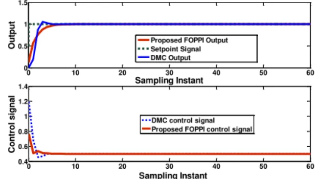
4.2 Example 2 – Non-Minimum Phase Control Comparison Consider a non-minimum phase process control example where the model is described using state space with matrices:
0.0217 0.3141 0.3141 ; = ; = 1 2 . 0.3141 0.7630 0.2364 A B C (Uren & Schoor, 2011)
The sampling period Ts is selected as 1s. Prediction horizon is
chosen to be 7 and fractional order of 0.9. The number of optimization steps is chosen to be 7 and all weight matrices chosen as unity identity matrices of proper dimension. Obtained control matrix is given:
12 0.5539 0.7005 0.6584 0.5142 0.3281 0.149 0.0252 0.1401 0.1772 0.1666 0.1301 0.0830 0.0377 0.0065 10 0.002 0.0003 0.0003 0.0002 0.0001 0.0001 0.0000 U x
With ki and kp equal to 0.15, excellent set-point tracking is
achieved as shown in Fig.2. In order to demonstrate comparative benefit, DMC is used as a baseline (Uren & Schoor, 2011). It was properly tuned for this same plant by the authors using Np =20; Nc = 3; Ts is selected as 1 and
weight R = 0.9I. The resultant (incremental) DMC control:
13 0.1503 10 0.0190 0.0479 mpc U x
Applied control signal is updated (u1u0 u1 ). Fig. 3 shows disturbance rejection property of these two controllers. A 25% input disturbance is introduced at 200s. It can be observed that the control input of the proposed fractional predictive controller falls within the range:0 u 0.8.
Fig. 2. Step response diagram showing the proposed output (brown) rising to the unit step reference with zero overshoot compared to DMC output (blue).
0 10 20 30 40 50 60 70 80 0 0.5 1 1.5 Sampling Instant O u tp u t 0 10 20 30 40 50 60 70 80 -0.02 0 0.02 0.04 Sampling Instant Co n tr o l s ig n a l Control Signal Setpoint signal Proposed FOPPI Output
0 10 20 30 40 50 60 0 0.5 1 1.5 Sampling Instant O u tp u t
Proposed FOPPI Output Setpoint Signal DMC Output 0 10 20 30 40 50 60 0.4 0.6 0.8 1 1.2 1.4 Sampling Instant Co n tr o l s ig n a l DMC control signal Proposed FOPPI control signal
Fig. 3. Disturbance rejection comparison – Both methods have similar settling time of 5s after 25% disturbance (green) is introduced at k=50s.The proposed method (brown) have zero overshoot.
6. CONCLUSIONS
It can be observed from simulation examples that the new fractional predictive control design method performs better than dynamic matrix control algorithm without any increased computational overhead. Also, control effort used to achieve this result is smaller therefore meeting any input constraints more easily. The significance of the proposed design is in simplicity of tuning. While the algorithm can be computed in some programmable or computerised fashion, the entire design procedure can be automated to the point of pushing kp and kI
knobs. This is expected to be attractive to industrial practitioners.
REFERENCES
Camacho, E. & Bourdons, C., 1998.
Model Predictive
Control.
London: Springer-Verlag.
Guo, W., Wen, J. & Zhuo, W., 2010.
Fractional-order
PID Dynamic Matrix Control Algorithm based on
Time Domain.
Jinan, China, IEEE.
Katebi, M. & Moradi, M., 2001. Predictive PID
Controllers.
IEE Proceeding - Control Theory
Applications,
148(6), pp. 478-487.
Lee, C.-H. & Chang, F.-K., 2010. Fractional-order PID
controller optimization via improved
electromagnetism-like algorithm.
Expert Systems
with Applications,
37(12), pp. 8871-8878.
Li, Z. & Chen, Y., 2014.
Ideal, Simplified and Inverted
Decoupling of Fractional order TITO Processes.
Cape
Town, IFAC.
Luo, Y., Chenc, Y. Q., Wang, C. Y. & Pi, Y. G., 2010.
Tuning fractional order proportional integral
controllers for fractional order system.
Journal of
Process Control,
20(7), pp. 823-831.
Luo, Y. & Chen, Y., 2009. Fractional order [proportional
derivative] controller for a class of fractional order
systems.
automatica,
Volume 45, pp. 2446-2450.
Miller, R., Shaha, S., Wooda, R. & Kwokb, E., 1999.
Predictive PID.
ISA Transactions,
Volume 38, pp.
11-23.
Monje, C., Vinagre, B., Vicente, F. & Chen, Y., 2008.
Tuning and auto-tuning of fractional order
controllers for industry applications.
Control
engineering practice,
16(7), pp. 798-812.
Padula, F. & Visioli, A., 2011. Tuning rules for optimal
PID and fractional order PID controllers.
Journal of
Process Control,
21(1), pp. 69-81.
Podlubny, I., 1999. Fractional-Order Sysmtems and PID
Controllers.
IEEE Transactions on Automatic Control,
44(1), pp. 208-214.
Song, X., Chen, Y., Tejado, I. & Vinagre, B. M., 2011.
Multivariable fractional order PID controller design
via LMI approach.
Milano, Italy, International
Federation of Automatic Control.
Uren, K. & Schoor, G., 2011.
Predictive PID control of
non-minimum phase systems,
Potchefstroom:
Intech.
Vale´rio, D. & Costa, J. S. d., 2006. Tuning of fractional
PID controllers with Ziegler Nichols Type Rules.
Signal Processing,
86(10), pp. 2771-2784.
Wang, L., 2009.
Model Predictive Control System
Design and Implementation with Matlab.
London:
Springer Verlag.
Zhuang, D., Yu, F. & Lin, Y., 2008. Evaluation of a
Vehicle Directional Control with a Fractional Order
PD Controller.
International Journal of Automotive
Technology,
9(6), pp. 679-685.
0 10 20 30 40 50 60 0 0.5 1 1.5 Sampling Instant O u tp u tProposed FOPPI Output Disturbance Signal DMC Output Setpoint signal 0 10 20 30 40 50 60 0 0.5 1 1.5 Sampling Instant Co n tr o l s ig n a l DMC Control signal