Marquette University Marquette University
e-Publications@Marquette
e-Publications@Marquette
Computer Science Faculty Research andPublications Computer Science, Department of
2018
MPI-Vector-IO: Parallel I/O and Partitioning for Geospatial Vector
MPI-Vector-IO: Parallel I/O and Partitioning for Geospatial Vector
Data
Data
Satish Puri Anmol Paudel Sushil K. Prasad
Marquette University
e-Publications@Marquette
Computer Science Faculty Research and Publications/College of Arts and
Sciences
This paper is NOT THE PUBLISHED VERSION;
but the author’s final, peer-reviewed manuscript.
The
published version may be accessed by following the link in the citation below.
ICPP 2018 Proceedings of the 47th International Conference on Parallel Processing
, No. 13 (2018).
DOI
.
This article is © Association for Computing Machinery and permission has been granted for this version
to appear in
e-Publications@Marquette
. Association for Computing Machinery does not grant
permission for this article to be further copied/distributed or hosted elsewhere without the express
permission from Association for Computing Machinery.
MPI-Vector-IO: Parallel I/O and Partitioning
for Geospatial Vector Data
Satish Puri:
Marquette University Milwaukee, WisconsinAnmol Paudel:
Marquette University Milwaukee, WisconsinSushil K. Prasad:
Georgia State University Atlanta, GeorgiaABSTRACT
In recent times, geospatial datasets are growing in terms of size, complexity and heterogeneity. High
performance systems are needed to analyze such data to produce actionable insights in an efficient manner. For polygonal a.k.a vector datasets, operations such as I/O, data partitioning, communication, and load balancing becomes challenging in a cluster environment. In this work, we present MPI-Vector-IO1 , a parallel I/O library
that we have designed using MPI-IO specifically for partitioning and reading irregular vector data formats such as Well Known Text. It makes MPI aware of spatial data, spatial primitives and provides support for spatial data types embedded within collective computation and communication using MPI message-passing library. These abstractions along with parallel I/O support are useful for parallel Geographic Information System (GIS) application development on HPC platforms.
Performance evaluation is done on Lustre and GPFS filesystems. MPI-Vector-IO scales well with MPI processes and file size and achieves bandwidth up to 22 GB/s for common spatial data access patterns. We observed that independent file read functions performed better than collective functions in MPI-IO for contiguous access pattern on Lustre. In general, the I/O is improved by one to two orders of magnitude over real-world datasets using up to 1152 CPU cores. Spatial Join query is used as an exemplar to demonstrate an end-to-end application using MPI-Vector-IO.
KEYWORDS
Message Passing Interface, Parallel IO, HPC, Spatial Join, Spatial Data
1 INTRODUCTION
In Geo-spatial domain, there has been a recent explosion in the amount of spatial data produced by satellites, medical and GPS enabled devices [25]. For example, NASA satellite data archive exceeded 500 TB and is still growing [10]. OpenStreetMap (OSM) data in a single XML file is about 800 GB [23]. However, the current software stack in spatial computing is rather ill-suited to the emerging realities of big data. In addition to “raster” format, polygonal spatial data are stored in a variety of “vector” data formats including ESRI Shapefiles, Well Known Text (WKT), OSM XML, CSV (New York Taxi dataset), etc [11, 13, 20, 22]. In this work, we
concentrate on vector data where shapes are represented with points, lines and polygons. The polygonal (vector) data are harder to process in parallel due to non-uniform distribution and irregular shape.
Spatial computing tasks like spatial join is both data- and compute-intensive. Spatial join is important in spatial data management systems to gain insights from large-scale geospatial data. Parallel I/O and spatial partitioning of irregular vector data (as opposed to raster data) is challenging and difficult to optimize. Real data distribution is often skewed. Spatial operations involve non-uniform data access and computation due to varying number of vertices in different shapes with no well-defined communication pattern due to irregular spatial task
distributions. Large polygons may have more than 100K coordinates. Optimizing such tasks in a heterogeneous parallel environment requires focus on efficient I/O, communication and computation. Many disaster response scenarios call for leveraging high performance computing techniques to yield real-time results e.g., in forest fire or hurricane simulation, where multiple layers of spatial data needs to be joined and overlaid to predict the affected areas and rescue shelters.
MPI-IO is a parallel I/O interface specified in the MPI-2 standard. It is implemented and used on a wide range of platforms. MPI has become the de facto parallel mechanism for I/O and communication on most high
performance computing systems. It provides contiguous and non-contiguous access patterns using independent and collective functions (Level 0 to 3). However, MPI only provides functions for unformatted binary file I/O. It does not provide functions for formatted text based spatial data which is the case with the vector data that we consider here in this paper [11, 22]. MPI-IO integration into existing geo-spatial HPC systems allows them to benefit from the optimizations built into the MPI-IO implementations.
An MPI based GIS system (MPI-GIS) to parallelize a spatial computation requires file partitioning and spatial partitioning of data among MPI processes. Using a parallel filesystem and I/O middleware for geo-spatial vector data has not been explored before. The I/O performance depends on file access patterns exhibited by an application. Design space exploration is needed to answer questions like how much throughput is achievable for irregular data access patterns on a given parallel filesystem. For this requirement, we have developed MPI-Vector-IO, a parallel I/O library using MPI-IO on top of parallel filesystem that can efficiently partition spatial data consisting of variable length geometries. The size of a geometry varies from less than a KB to more than 10 MB. We have implemented three levels of MPI-IO abstractions and evaluated them on GPFS and Lustre. We also
study contiguous and non-contiguous access patterns and their ramifications on performance and spatial partitioning. Spatial join is chosen as an exemplar application for end-to-end evaluation.
We discuss the design and implementation of a user-friendly I/O and partitioning library targeted to GIS community’s need to run spatial analytics on an HPC platform. MPI-Vector-IO is not tied to any specific format. This library improves the state of the practice by enabling HPC based GIS systems to handle publicly available datasets where a single file can be more than hundred GBs in size. MPI-Vector-IO introduces spatial data aware abstractions for collectives in MPI and provides communication interfaces required for global spatial
partitioning. It can perform I/O and parsing for a variety of data types including polygon/polyline. Two
approaches have been designed for file partitioning in order to ensure that a geometry does not get split among consecutive MPI ranks.
The main contributions of this paper can be summarized as follows:
(1) MPI-Vector-IO: Parallel I/O support for partitioning and reading variable length geometries using MPI-IO. By using a flexible interface, it allows user-defined methods to parse coordinates to GEOS geometry objects. We provide benchmarks for contiguous and non-contiguous access patterns on Lustre and GPFS parallel filesystems.
(2) Evaluation of independent and collective MPI file read functions. We show that independent
functions provide better performance than collectives for contiguous file read operations on vector data stored on Lustre.
(3) Spatial data aware MPI: Derived spatial data types, spatial reduction operations and communication support for spatial data using MPI. With these new spatial types, the efficiency of built-in reduction operations can be leveraged.
(4) An MPI framework to parallelize spatial computations on top of MPI-Vector-IO (described in Section 4.3). The framework enables parallel spatial indexing and join operations on an order of magnitude larger datasets (indexing up to 700M geometries in 137 GB single file in 90 seconds) [1–3, 5, 27, 28, 32]. The rest of the paper is structured as follows. Section 2 presents general technical background related to this paper. Section 3 discusses the challenges and implementation issues. In Section 4, we present the design and implementation details of MPI-Vector-IO. Section 5 presents the experiments and evaluation using real datasets. Section 6 concludes this paper.
Level 0 Contiguous and Independent Level 1 Contiguous and Collective Level 3 Non-contiguous and Collective Table 1: Three levels in MPI file read functions.
2 BACKGROUND CONCEPTS AND RELATED WORK
Vector data:Well-Known Text (WKT) is a text markup language for representing vector geometry objects on a map. A polygon with 3 vertices is represented as POLYGON ((30 10, 40 40, 20 40, 30 10)) [31]. Its binary equivalent, known as Well-Known Binary, is used to transfer and store the geometries in spatial databases. These formats were originally defined by the Open Geospatial Consortium.
Parallel I/O and MPI-IO: Parallel filesystems like GPFS and Lustre store chunks of a file across multiple hard disks which make parallel read/write possible. In Lustre, stripe count and stripe size can be specified for a file and a directory. Stripe count means the number of storage devices (OST) where the file blocks are striped. MPI provides I/O routines for read/write operations by multiple processes to a common file. Using parallel I/O can
lead to improved performance and provides a single file for storage and transfer purposes. File access can be expressed in contiguous or non-contiguous fashion (each process accesses multiple small chunks of data located noncontiguously). Special functions like MPI_Type_contiguous and MPI_Type_vector can be used for non-contiguous types. These types allow for gaps such that elements are separated by multiples of the extent of the input datatype. An example of non-contiguous area is a column of a 2D array stored in a row major order. MPI provides independent and collective functions for file read and write operations as shown in Table 1.
In literature, there are several studies and software tools like PnetCDF, HDF5, ADIOS, T3PIO, HieRO, etc. for optimizing I/O in an HPC environment [8, 15, 18, 19, 21, 24]. These are geared towards scientific and simulation applications reading/writing checkpoint or visualization data and use specific file formats like NetCDF, HDF, BP, etc. These formats are very different from spatial vector data formats. Using the existing libraries mentioned earlier would require data format conversion and preprocessing to store file offsets of the variable length geometries in order to allow random access for partitioning. Our proposed method (Algorithm 1) uses interprocess communication to partition the file on the fly and does not require any preprocessing. Some file access patterns in GIS are also different from scientific applications. Chou et al. discusses in-memory system for spatial indexing and query without using a parallel filesystem [8]. Our work is geared towards spatial data analytics use cases where the data resides on a parallel filesystem.
Much of the research on big spatial data has been done on top of HDFS filesystem using MapReduce paradigm [4, 12]. The default design of HDFS/Hadoop cannot efficiently utilize the advanced features of the available resources in HPC platforms. In our past project on polygon overlay computation, we found MPI-based system to be faster than Hadoop based system [26]. With time-critical and latency sensitive applications in mind, we are proposing HPCoriented solution to geo-spatial data problems based on MPI.
Geometry Engine OpenSource (GEOS) is a widely used C++ library that provides 1) spatial data structures including Quadtree and R-tree, 2) computational geometry and GIS algorithms, and 3) parsing WKT geometries.
MPI-Vector-IO internally calls this library for geometric algorithms. Due to this integration, it enables the usage of GEOS in a shared-nothing MPI environment.
Filter and Refine technique: Spatial query e.g. searching for all geometries overlapping with a polygon p is carried out in two phases. In the filter phase, all of the spatial data is scanned and overlap test is carried out with
rectangular approximation (bounding rectangle) of the geometries. Using approximations produce some false positives. Therefore, in the refine phase, actual geometries are used for overlap test. This technique leads to better performance because overlap test on rectangles is faster than with the larger and complicated geometries. Moreover, a sizable chunk of the input geometries are weeded out in the filter phase itself.
By combining the generality of filter and refine with the GEOS library, a framework can be developed to handle a class of spatial analytics use cases. We will show how to combine this framework with MPI-Vector-IO for
parallelization in Section 4.3 and show spatial join as an exemplar.
Spatial Join: Spatial join is similar to join operation on two tables in a database. In spatial join, the records have spatial attributes i.e. 2D objects and the join operation is defined on spatial properties. An example of a spatial join is “Find all pairs of rivers and cities that intersect.” Intersect operation for a given pair of polygons returns true if and only if polygons share any portion of space. In general, spatial join can be defined as follows: given two spatial datasets R and S and a spatial join predicate θ (e.g., overlap, contain, intersect) as input, spatial join returns the set of all pairs (r,s) where r ∈ R, s∈S, and θ is true for (r,s) [16]. Similar to spatial queries, spatial join also follows filter and refine technique.
Existing MPI based approaches: There are few HPC based research studies focused on parallelizing spatial computations on CPU and GPU without much attention to parallelize file I/O [3, 5, 32]. Our earlier work on
polygon overlay avoided file partitioning and it was not designed to use any parallel filesystem [1, 28]. As such, file I/O proved to be the bottleneck. Each process read a chunk of input shapefile using a sequential library. This approach only worked with a shapefile because it maintains an extra index file to hold the offsets of the
geometries in the main file. For other XML data formats, we implemented redundant file reading by all
processes and master process distributing data to other workers. These redundant and serial I/O strategies were slow, cumbersome, and overwhelmed the memory capacity of individual nodes for larger data. Other research projects do not study the parallel I/O issues for variable length spatial data [5, 8].
3 CHALLENGES AND IMPLEMENTATION ISSUES
Users in geo-spatial domain are tool constrained in HPC environment. For large geo-spatial files, data partitioning is one of the big challenges. Following questions are addressed in this paper:
1) Data Partitioning: How to partition a file that contains irregular and unstructured data (co-ordinates + attributes)? Simple partitioning by file-blocks fails due to geometries getting split across two consecutive MPI ranks.
2) Expressing vector data I/O using MPI: MPI-IO functions are for unformatted binary file access similar to POSIX
read and write functions [14]. Using these functions require reading the file, followed by parsing phase to construct data types. MPI does not have any functions for formatted text I/O equivalent to fprintf and fscanf in C language. Formatted I/O functions are suitable for text-based spatial data; for instance, parsing phase is not required for reading points, lines and rectangles using fscanf. Given the fact that MPI-IO functions are designed for binary unformatted data, how to use them effectively for geo-spatial applications where the data is
formatted and not necessarily in binary form? A variety of geometry representations defined by Open Geospatial Consortium should be supported and the nitty-gritty of file and data partitioning issues should be abstracted away by the parallel library.
3) MPI-IO and ROMIO issues: MPI standard specifies that the count parameter passed to MPI functions be a 32-bit integer. Using user-defined derived data types, count can be reduced to a lower number than what a 32-bit integer can hold. However, this creates problem with ROMIO, a widely used MPI-IO implementation, where an MPI process can not read/write more than 2 GB of data in a single operation. It should be noted that this is a known limitation of ROMIO. For MPI communication of large data, derived data types are not sufficient for irregular MPI collectives. For instance, in Alltoallv that allows processes to send messages of different sizes, but have only one datatype parameter, a single derived data type that will work for all processes needs to be defined at run-time. This requires additional phase of communication to determine the extent of the new data type a priori. With respect to the new data type, the communication buffer needs to be padded accordingly, which adds overhead during serialization and deserialization.
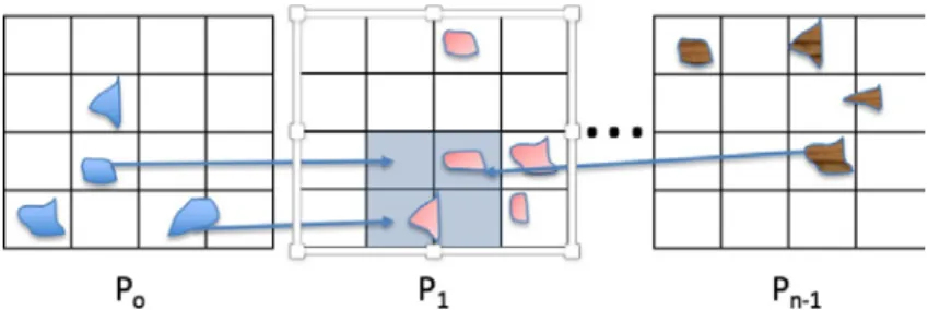
Figure 1: Local geometries read by MPI-Vector-IO is projected to a grid by each process. Shaded area represents tasks assigned to 𝑃𝑃1. For spatial locality, 𝑃𝑃1 needs geometries overlapping with its area from other processes
4 MPI-VECTOR-IO
In this section, we will discuss data parallel MPI-Vector-IO architecture with respect to I/O, file and spatial partitioning using MPI.
For efficient and scalable partitioning of vector data, we need to focus on all three aspects - I/O, computation, and communication. In order to parallelize spatial computations, MPI-Vector-IO performs data partitioning in two distinct phases - 1) file partitioning for data parallelism and 2) cellular grid based partitioning to ensure spatial locality.
Two access patterns are used depending on the size of the data and application. For large files, a block size needs to be specified with an upper bound of 2 GB per process due to ROMIO limitation. Block size can be varied by user to control the granularity of computation. If block size is not defined, then the file is logically divided equally among the processes. After file partitioning, each process reads the local geometries and projects them to a local grid as shown in Figure 1. Inter-process exchange of geometries is required to get a global partitioning of the overall data in order to ensure that each cell of the grid contains all the geometries that lies in it partially or completely. If a geometry spans multiple cells, then it is simply replicated to these cells. Duplicate avoidance is carried out later in the refinement phase. The data decomposition is in terms of cell which is also an abstract type to represent a unit task in our system. A subset of these cell-based tasks are assigned to processes.
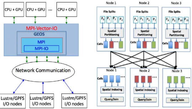
MPI-Vector-IO system carries out filter-and-refine on spatial data stored on parallel filesystem in a distributed fashion. Figure 2 shows the architecture and data flow in a cluster environment with high performance
interconnects and parallel filesystems. The general architecture shown in this figure represents the data flow for a range of applications like spatial query, join and overlay. The data flow diagram shows distributed spatial computation and communication using 3 compute nodes. The geometries in a file partition (𝑃𝑃0 to 𝑃𝑃11) are
mapped to corresponding grid cells. For populating the cells with geometries overlapping with its boundary, an R-tree is first built by inserting the individual cell boundaries. Then, for each geometry in the local file partition, the overlapping grid cells are determined by querying with the geometry’s MBR against this R-tree. An all-to-all personalized data exchange produces global spatial partitioning.
We start with our main contribution - parallel I/O and partitioning for polygonal data. Then, we will show how to parallelize spatial computations on top of MPI-Vector-IO.
Figure 2: MPI-Vector-IO architecture and data flow diagrams.
4.1 Design and implementation of
MPI-Vector-IO
Depending on the type of spatial data, MPI-Vector-IO supports both formatted as well as unformatted data. It takes advantage of the I/O interface in MPI that supports features like collective and independent I/O. The input layers are split into logical partitions among MPI processes. For text-based data like WKT, each file partition is treated as collection of strings and assigned to a single process. All the strings in each partition gets parsed into geometries first and then mapped to one or more grid cells based on its MBR’s spatial overlap with the grid cells.
Figure 3: File partitioning among processes (contiguous mode).
Contiguous File Access: In MPI-Vector-IO, the basic idea is to logically partition the entire file among N processes. Each process participates in reading a portion of a common file as shown in Figure 3. For formatted text data, default file view is used for contiguous file access. In order to handle data with co-ordinates and text attributes, we have used buffer of MPI_CHAR data type in MPI-IO functions. A user can select the I/O functions to be used in independent (Level 0) or collective (Level 1) mode by each process. If block size is not specified, then each process reads equal chunks of the file as shown in Figure 3. Otherwise, each process determines the file offsets based on the block size specified by the user. The block size is defined for each process. In this case, there are multiple iterations of file access required to read the complete file. As shown in Algorithm 1, all iterations except the last one read (N*blockSize) bytes. The last iteration requires special handling. Depending on the portion of file remaining in the last iteration, a subset of processes call the file read function.
Handling variable-length geometries: Due to file partitioning, a polygon vertex list can potentially get split across file partition read by a process. This is undesirable since a shape needs to be read by one process in its entirety. To prevent this splitting, a process needs to read slightly more than (FileSize/N) bytes. The exact number of bytes is determined by the maximum size of a shape in our current data sets which is 11 MB to handle the largest polygon. One way to resolve this issue is to allow the file access by two consecutive processes to overlap with each other near the block boundaries. This overlap area is similar to a halo region and its length can be specified if the upper bound on the size of a geometry is known a priori. Among the two contending processes, one of them needs to take the ownership of the geometry spanning a block boundary. This approach requires
O(N) bytes of redundant file reading because of overlapping read accesses. This problem is further exacerbated when multiple iterations are required to read the file completely because the block size read by each process is small.
Dynamic file partitioning: Another approach is to read fixed-size blocks with no overlaps by each MPI process and use send and recv communication in a ring fashion where an MPI process passes the incomplete geometry’s co-ordinates to its neighboring process as shown in Algorithm 1. MPI communication is used instead of MPI processes reading overlapped file blocks. In Line 12 of Algorithm 1, the processes are partitioned into two groups to avoid deadlock conditions. One group consists of even-numbered processes and the other of the numbered processes. The even-numbered processes perform a send followed by receive, and the
odd-numbered processes perform a receive followed by a send. Only three arguments are shown in the send/receive function calls, namely buffer address, buffer size and source/destination ranks. In Line 15 and 17, the receive function’s max buffer size is fixed as 11 megabytes. To get the actual number of data types received,
MPI_Get_count function is used. If an upper bound on the message size is not easy to calculate, MPI Probe and Get_Count functions are required to find the message size for receive function’s buffer allocation. Dynamic file partitioning solves the variable length geometries getting split among processes. This approach does not require
halo regions and has the advantage of not doing redundant file reading. Moreover, parallel file read access will be stripe aligned.
Figure 4: File partitioning (non-contiguous mode). Each process reads file partitions in a round-robin fashion.
Non-Contiguous File Access for Spatial Data: In many GIS applications, the co-ordinate data is partitioned among grid cells and the cells are distributed among MPI processes in a round-robin fashion for load-balancing. For example, in a grid-based polygon overlay operation, the output needs to be written to a single file in which the storage order corresponds to that of the global grid data layout in row-major order. Since the spatial data is distributed among processes, this requires non-contiguous file writing (shown in Figure 4). This ensures that the output file is same as if produced sequentially.
To ensure spatial data locality, points and line segments are often sorted in 2D using Z-order and Hilbert curve. Rectangles and polygons are partitioned into grid cells for the same purpose. For spatially sorted data,
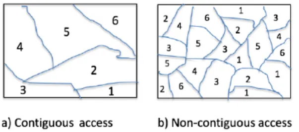
contiguous and non-contiguous file reading results in different partitioning. A contiguous access may result in coarse-grained and uneven spatial partitioning among different processes as shown in Figure 5 a) with 6 processes. For skewed data, this may lead to load-imbalance among processes. Non-contiguous read creates fine-grained tasks and declustering of data as shown in Figure 5 b). Heuristics like declustering geometries and round-robin assignment to tasks has been shown to be effective for load-balancing [30]. By defining custom file
views using derived data types, MPI-Vector-IO enables these techniques to be applied while doing file read for point, line segment, and polygonal data.
Figure 5: Spatial partitioning as a result of file partitioning among 6 processes with a) default file view (Figure 3) and b) non-contiguous file view (Figure 4).
Algorithm 1 Iterative File Reading - Message based 1: Input variables: fileSize, blockSize, N, rank 2: MPI_Offset globalOffset ← 0
3: MPI_Offset fileChunkSize ← N * blockSize 4: iterations ← [fileSize/fileChunkSize] 5: for (i=0; i <(iterations-1); i++) do
6: globalOffset ← i * fileChunkSize 7: start ← globalOffset + rank * blockSize
8: MPI_File_read_at_all(file, start, fileBuffer, blockSize) 9: lastDelimPos ← blockSize-1
10: while (fileBuffer[lastDelimPos] != DELIMITER) do
11: lastDelimPos-- 12: if (rank%2 == 0) then
13: MPI_Send((fileBuffer+lastDelimPos), 14: (blockSize-lastDelimPos), (rank+1)%N)
15: MPI_Recv(recvBuffer, maxBufferSize, (rank-1+N)%N) 16: else
17: MPI_Recv(recvBuffer, maxBufferSize, (rank-1+N)%N) 18: MPI_Send((fileBuffer+lastDelimPos),
19: (blockSize-lastDelimPos), (rank+1)%N) 20: handleLastIteration()
Unlike polygons that vary in length, spatial types like points, lines, and MBRs have fixed length. Files containing these special types are preprocessed and stored in binary as basic or struct type. MPI-IO functions then directly read the data as MPI datatypes. In case of spatial index files that need frequent access, the advantage in doing so is that file access becomes regular and much faster. Moreover, custom file views can be easily defined for these unformatted files with fixed-size records. This makes non-contiguous file access easier to implement. A file block size needs to be defined in terms of number of datatypes to specify the areas in file accessible per process. Implementing non-contiguous file access for variable length polygons and polylines requires preprocessing. Vertex count and displacement arrays containing length of geometries and arrayoffsets are populated as a preprocessing step. Using these auxiliary arrays, MPI_type_indexed derived data type is created to specify block layout in file views. Collective functions are used in all cases.
Spatial Type Spatial Reduction
MPI_POINT MPI_MIN RECT, LINE, POINT
MPI_LINE MPI_MAX RECT, LINE, POINT
MPI_RECT MPI_UNION RECT
Table 2: Spatial data types and reduction operators.
Figure 6: Using new types and operators in MPI functions.
4.2 Collective Computation and Communication for Spatial types
This subsection is motivated by the fact that user-defined data types and operations not only enhance the abstraction and reusability of a system, but also performance in case of MPI in the presence of hardware support [6]. Using derived datatypes and functions to specify the data layout, non-contiguous elements need not be copied to additional buffer for send/recv and file access operations, thereby, leading to optimized communication. In case of I/O, it may lead to fewer system calls and physical disk I/O.
4.2.1 Spatial data types.
MPI provides a rich set of predefined datatypes. Using these, we have defined additional derived types to represent spatial data that are supported by WKT and GEOS library e.g., MPI_Point, MPI_Line, MPI_Rect, etc. These data types are shown in Table 2. For instance, MPI_Rect is defined as a contiguous type of 4 doubles. Additional compound types such as multi-point, multi-line, and fixed-size polygon are defined by nesting basic spatial types. With these new spatial types, the efficiency of built-in MPI reduction operations can be leveraged, provided we define new reduction operators for the corresponding data type using MPI_Op_create and pass it to the user-defined function. An example showing how to use it is given in Figure 6.
4.2.2 Collective Reduction Operators for Spatial types.
With derived data types, existing MPI reduction operators like MPI_MIN, MPI_MAX, etc., do not work. So, we have redefined them for lines, MBRs, etc. The min operator can be used to find the line or rectangle with
minimum size among processes. New MPI_UNION operator on MBRs is also defined which has been used to find the grid dimensions from the union of MBRs generated by individual processes during spatial partitioning. To implement it, there is a user-defined function linked to the union operator that performs geometric union of rectangles. MPI uses this operator to carry out the function in a optimized reduction tree fashion. An example usage is shown in Figure 6. These operators can be non-commutative, but must be associative.
4.2.3 Communication buffer management.
There are two inputs to this module for each MPI process - 1) the spatial data read from a file partition that is already mapped to a cellular grid and 2) rankto-cells mapping, for example, round-robin. Since a process may have a geometry belonging to a cell mapped to a different process, data exchange is required for global spatial partitioning. MPI bufferoriented communication requires serialization and deserialization of geometries (grouped by cell) by each process. Each MPI process serializes the coordinates and geometry related text data for all MPI processes in its send character buffer for all-to-all exchange. For vector data consisting of polygons, the number of vertices vary considerably. MPI-Vector-IO provides collective communication functions to exchange spatial data of different types (including polygons) among processes. Due to the variation in the number of geometries and size of each geometry to be sent (received) to (from) other processes, each MPI process needs to provide send (recv) count and displacement arrays. As such, all-to-all collective communication
is performed in at least two communication rounds. Before actually sending the entire co-ordinate data using
MPI_Alltoallv, the processes exchange the buffer related information among them using MPI_Alltoall which is then used to calculate the receiver side count and displacement arrays of MPI_Alltoallv.
Handling large data exchange: For large data sets, it is often not possible to perform data exchange in a single phase due to memory limitations. As such, we have incorporated sliding window technique where
communication happens in distinct number of phases in an iterative manner. In each phase, spatial data contained in a chunk of cells are exchanged.
4.3 Parallelizing Spatial Computations using
MPI-Vector-IO
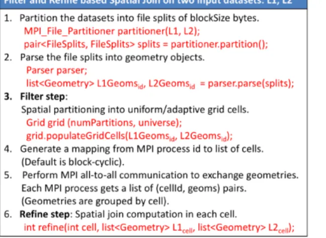
Many GIS applications involving query and join operations require a filter-and-refine approach. As such, MPI-Vector-IO extends this concept to be carried out in a distributed fashion. As a system, MPIVector-IO is designed in an extensible manner to take care of file splitting and spatial partitioning using object-oriented approaches to handle a variety of data formats with minimal change. Basic steps required to parallelize spatial computations are shown in Figure 7.
Parsing module: Spatial data is parsed while reading the file from disk and from the MPI communication buffer during deserialization. Unlike PnetCDF, our implementation is not tied to any specific file format. To handle a variety of file formats, our flexible interface presents the geometric data in those files as a collection of strings, thereby allowing user to define parsing method that returns a GEOS geometry for each string. For reading WKT data format, the parse interface is implemented by WKTParser class that extracts the coordinates by parsing them into Geometry objects. This extensible approach applies to other vector data as well e.g., XML and CSVbased spatial data. Other feature data associated with the geometry is stored in userdata field of GEOS Geometry class. Using GEOS library internally allows our system to represent a wide variety of shapes defined by OGC standard.
Figure 7: Main steps for performing spatial computation using MPI-Vector-IO.
For partitioned data, spatial computation can be carried out by extending refine interface that receives two collection of geometries in a cell. For spatial query workload, the second collection can be treated as geometries from batch query. Refine tasks are scheduled based on the task mapping across processes thereby carrying out distributed spatial computations in different cells. More details on the library with examples are provided on the project page 2.
5 EXPERIMENTAL RESULTS
This section provides an experimental study of the performance of our system using a variety of large vector datasets. First, as our contributions are about spatial data support in MPI, the experiments are designed to show
the performance of the various system components. We have chosen spatial join as a representative application. We have not compared MPI-Vector-IO with PnetCDF or ADIOS. Using these tools would require cumbersome conversion of the real vector datasets to tool-specific formats and preprocessing to calculate the file offsets for each geometry in order to allow random access.
Table 3: Real-world datasets and Sequential parsing time.
Dataset Shape File Size Count I/O (sec)
1 Cemetery Polygon 56 MB 193 K 2.1
2 Lakes Polygon 9 GB 8 M 328
3 Roads Polygon 24 GB 72 M 786
4 All Objects Polygon 92 GB 263 M 4728 5 Road Network Line 137 GB 717 M 2873
6 All Nodes Point 96 GB 2.7 B 3782
Parsing large datasets: Spatial data sets are growing in size. Table 3 shows the description of the datasets with different sizes, types, and number of shapes extracted from OpenStreetMap which represents map data from the whole world [22]. For spatial queries on large spatial data files of 100 GBs, I/O and parsing phase itself takes about an hour, as shown in the last column of the table.
Cluster Information: We have used COMET cluster with Lustre filesystem [9]. The cluster has 2.5 GHz Intel Xeon E5-2680v3 processors and 128 GB DDR4 DRAM. Each node has 24 cores. The network topology is FDR InfiniBand with 56 Gb/s link bandwidth. It has 6 petabytes of 100 GB/s durable storage. There are 96 OSTs available for striping. Maximum compute nodes that are allowed in a single job is 72. 16 MPI processes are run per node. We used Open MPI version 1.8.4 and GCC 4.9.2.
We have used ROGER cluster [29] with GPFS parallel filesystem. The compute nodes have two Intel Xeon E5-2660 v3 chips. Each chip has 10 cores, each running at 2.6GHz. Each node has 256 GB of physical RAM. The cluster is connected by a high-speed network with 40Gb/s switches in the core and 10Gb/s uplinks to each node. 20 MPI processes are run per node. We used MPICH/3.1.4 and GCC 4.9.2 to build the system. GEOS library version 3.4.2 has been used for local spatial indexing and join [17].
First, we evaluate MPI-Vector-IO on Lustre and GPFS. Then, in subsection 5.2, we evaluate an end-to-end spatial join system built on top of MPI-Vector-IO.
5.1
MPI-Vector-IO
performance evaluation
The results shown here are average of at least three runs. First, we discuss performance evaluation of file read operations (Level 0 and 1) on Lustre by varying stripe count (OST) and stripe size. On GPFS, we did not have the permission to change those parameters. Therefore, we used the default filesystem configuration on GPFS.
5.1.1 Lustre Experiments.
The granularity of spatial computation can be controlled by varying block sizes to be read by each process. A user can specify coarse-grained block size if the application is less compute intensive e.g. range query. However, spatial join requires fine-grained block decomposition since it is very compute intensive. Moreover, grain size also impacts load balancing. Therefore, here we show how much throughput is achievable for a variety of block sizes.
In the following experiments, 16 cores per node is used with 1 MPI process for each core. A single file is striped using different stripe count (upto 96 OST allowed) and stripe size to study the performance variations. Block size read by each process is kept same as the stripe size for file access alignment with the stripes.
Performance of Algorithm 1 depends on the number of iterations of file access required to read a whole file in blocks. The number of iterations depend on the number of processes, file size, and block size read by each process (see steps 3 and 4 of Algorithm 1). For instance, in case of Roads data set, using 256 processes and 32 MB block size, 4 iterations are required to read the complete file. Using 16 MB block size, 7 iterations are required. However, if we use 128 processes and 32 MB block size, file read functions are invoked 7 times. Each time 4 GB file chunks are read and the file offset is advanced accordingly. In the last iteration, only 168 MB needs to be read. Therefore, the block size used for the last iteration is different than 32 MB. It should be noted that fewer iterations also means less send/recv messages to handle the geometries getting split among
consecutive MPI ranks.
Independent Read (Level 0): In Figure 8, file read performance in the order of GB/s is shown for the largest polygonal data. The number of nodes is varied from 4 to 72 (maximum allowed). The performance improves when the number of processes is increased up to a certain extent due to the reduction in the number of file access. For all stripe counts, there is a range of processes where relatively high bandwidth is achieved. The maximum bandwidth achieved is 22 GB/s using 48 compute nodes. In Figure 9, file read bandwidth for Roads data is shown for different number of OSTs. Roads is much smaller data set than All Objects. Therefore, we have chosen a smaller stripe size (32 MB) to allow larger number of processes in this experiment. Block size read impacts the I/O performance and with smaller size, we can see up to 8-9 GB/s bandwidth for different number of OSTs. In Lustre, performance for a given number of processes generally increases with the number of OSTs before reaching maximum value. The higher I/O requirement for larger number of processes quickly saturates the link bandwidth.
Figure 8: File Read bandwith for All Objects (92 GB) with stripe size 64 MB and128 MB. Stripe count 64 (Level 0).
Contiguous and Collective Read (Level 1): We compared the performance of reading Lakes (9 GB) by employing two strategies - 1) overlapping file access by consecutive MPI ranks and 2) nonoverlapping file access with send-recv communication (referred to as message based) to handle file partitioning for variable length geometries. As shown in Figure 10, message based algorithm performs better for a range of processes and stripe counts. Block size was fixed to 32 MB. We repeated this experiment on NFS filesystem as well with different block sizes and reached to the same conclusion. The overhead of reading 11 MB halo region by each process is greater than exchanging missing co-ordinates. Therefore, we have used message-based file partitioning for Level 0 and 1 access patterns.
Figure 9: File Read bandwith for Roads (24 GB) for different stripe counts and fixed stripe size 32 MB (Level 0).
Figure 10: Performance comparison between Message vs Overlap access strategy for three different stripe counts (OST).
Figure 11: File Read time for Roads (24 GB) with stripe size 16 MB (Level 1).
Figure 11 shows the read performance for Roads using three stripe counts and 16 MB block size. The maximum bandwidth achieved is 3.5 GB/s with 96 OSTs. For Lakes (9 GB), the maximum bandwidth achieved is about 3.6 GB/s with the same number of OSTs. When we doubled the block size to 32 MB, up to 5 GB/s bandwidth is achieved. For both datasets, performance improved with using higher stripe counts (OST). In general, for a fixed block size, disk access frequency and message passing overhead decreases when the number of processes increase. However, in the figure, we can see the performance drop for 24, 48, and 72 nodes. For instance, performance using 48 nodes is worse than 32. Similarly, performance using 24 nodes is worse than 16 nodes. This is due to the fact that on Lustre, the upper bound on the number of MPI processes actually performing read operation (reader) is equal to the number of nodes. The actual number of readers can be less than the number of nodes as described in the next paragraph.
MPI hint with key cb_nodes can be provided by the user to set the number of nodes performing I/O operations. However, on Lustre, the actual number of readers is determined based on whether the number of nodes is a multiple or a divisor of the stripe count [21]. We notice good performance when the number of readers selected by ROMIO is equal to the number of nodes. This happens when the stripe count (OST) is a multiple of the
number of nodes. This is shown in Figure 11 for 16, 32, and 64 nodes. The number of readers selected by ROMIO is a function of number of nodes and stripe count. When the stripe count is greater than the number of nodes, then the number of readers selected is equal to the largest divisor of stripe count that is less than or equal to the number of nodes. For instance, only 16 readers are selected when 24 nodes are reading from 64 OSTs3 .
When 48 nodes are reading from 64 OSTs, 32 readers are selected4 . This explains the performance drop for 24
and 48 nodes as shown in the Figure. So, for collective read functions to perform well the combination of node count and stripe count should be chosen appropriately such that the number of nodes should be a multiple or divisor of the stripe count. This issue has been reported for write performance on Lustre [21].
In general, independent functions performed better than collective for our block-based contiguous file read use case due to the overhead involved in collectives. For collective functions, I/O happens in two distinct phases. Only a subset of MPI processes (a.k.a. aggregators) perform I/O on behalf of the other processes. Then the
aggregators distribute the data to other processes using MPI_Alltoallv. For larger block size, the two phase I/O algorithm is split into multiple cycles due to buffer size constraints [7]. This leads to sub-optimal performance. We tried different values for cb_buffer_size and cb_block_size in order to tune collective buffering. However, the difference caused by these hints was not noticeable.
5.1.2 GPFS Experiments.
All the experiments in this subsection were performed on ROGER cluster. The last column in Table 3 shows the sequential I/O time for a variety of datasets. File I/O time depends on size of the dataset. However, the parsing time depends on the type of shape and the number of geometries in a dataset. For instance, polygonal data (All Objects) takes more time for parsing than line data (Road Network) as shown in the table, even though Road Network is larger in size than All Objects.
Figure 12 shows performance impact of MPI data types on reading binary file in contiguous mode.
MPI_Type_struct performs better than MPI_Type_contiguous. The difference is that in case of the struct, MPI implementation internally creates the C struct based on the data type definition whereas in the contiguous case, user code creates a C struct using 4 contiguous floating point numbers.
Figure 13 shows the performance for new MPI_Op for geometric Union using 100K, 200K and 400K rectangles. This operator is used in our system to get the global spatial grid dimensions by the union of local grid
dimensions.
Figure 13: MPI Reduce and Scan for geometric Union.
Figure 14: I/O+Parsing performance for All Nodes (96 GB) and All Objects (92 GB) on GPFS (Level 1).
Figure 14 shows the file reading performance for All Nodes and All Objects using contiguous access mode. Both files are about the same size but All Objects takes more time because parsing polygons take more time than point data in All Nodes. The I/O performance scales up to 80 processes for both files.
Non-contiguous and Collective Access (Level 3): Figure 15 shows binary unformatted file reading time for
contiguous and non-contiguous access modes. The block sizes show the number of MBRs where an MBR consists of 4 floating point numbers. As we can see in the figure, file access in contiguous mode is much faster. MPI-IO implementation has to perform more work in case of non-contiguous access in terms of interprocess
communication involved in twophase I/O. For non-contiguous mode, larger block sizes perform better due to less aggregation and communication overhead.
Figure 15: Binary file (10 GB) reading time for noncontiguous (NC) access modes on GPFS (Level 1 and 3). Figure 16 shows file reading performance for polygonal data using contiguous and non-contiguous access modes. In case of irregular and formatted data as well, contiguous access mode performs well and improves with increase in the number of processes for both datasets. However, performance of non-contiguous access is very sensitive to block-size and number of processes. The block sizes are specified in terms of number of
polygons in this figure. Since polygons vary in length widely, the I/O request per process is very irregular and can vary considerably with change in block size and number of processes.
Figure 16: Non-Contiguous (NC) I/O for polygon data with different block sizes on GPFS.
5.2 End-to-end performance evaluation
All the experiments in this subsection were performed on ROGER cluster. Here, we will discuss the component-wise performance breakdown with respect to partitioning, communication and computation phases for spatial join workloads. The partitioning time includes the time taken to populate the grid cells with the geometries read from a local file partition. The communication time includes the buffer management overhead in serialization, deserialization and exchange of geometry objects. The join time includes time for spatial indexing and geometric intersection test. In the following plots, we note the time taken by each process and take the maximum time for each of the components.
The effect of grid-based spatial partitioning can be seen in Figure 17. As the number of grid cells increase, the overall execution time decreases. The load in terms of number of geometries across cells can vary. Moreover, the cell to process mapping also changes as the number of grid cells and processes increase. This affects the load per process which reflects in the communication time. The total time is less than the sum of different phases because here we report the maximum time among all processes for each phase.
Figure 17: Execution time breakdown for different number of grid cells for Spatial Join (Lakes, Cemetery) using 80 MPI processes.
Figure 18: Execution time breakdown for spatial join (#2, #1).
In Figure 18, the spatial join time dominates the overall execution time. With increasing number of processes, the join time decreases as well. In Figure 19, the communication cost dominates the overall execution time. The execution time breakdown of different phases for in-memory spatial indexing of Road Network(137 GB) is shown in Figure 20. The performance of all the components improves with increase in the number of processes. Using 320 processes, spatial indexing of 717M edges takes only 90 seconds.
Figure 19: Execution time breakdown for spatial join (#3, #1).
Using end-to-end spatial join as an exemplar, we have shown that MPI-Vector-IO can handle data and compute-intensive spatial operation on an order of magnitude larger data sets. This has been made possible by our proposed parallel I/O and data partitioning approach. However, more work is required to improve the overall scalability of the system by incorporating dynamic load balancing. Data partitioning and communication can be further improved by making it locality-aware. Previous work in this area have only used few shapefiles where each file can only be 2 GBs [1, 5, 28, 32]. Hence, the current work improves the state of the practice in HPC GIS domain.
Figure 20: Execution time breakdown for indexing 137 GB (Road Network) among 2048 grid cells.
6 CONCLUSIONS
Analyzing large amounts of spatial data to guide decision making has become essential to businesses as well as scientific discovery. A spatial data framework for HPC environment needs parallel I/O and partitioning support for large scale collection of variable length geometries. In this paper, we introduced MPI-Vector-IO which enables HPC based GIS to handle large vector datasets of different formats efficiently. Introduction of new derived types for spatial data and reduction operators for spatial primitives make MPI spatial-aware. Moreover,
MPI-Vector-IO system takes care of file and space partitioning along with data communication under the hood, thereby, making it easy to use for spatial data computations in HPC environment. Going forward, we intend to integrate our GPU based work [3] with MPI-Vector-IO.
ACKNOWLEDGMENTS
This work is partly supported by the National Science Foundation Grant No. 1756000.
REFERENCES
[1] Dinesh Agarwal, Satish Puri, Xi He, and Sushil K Prasad. 2012. A system for GIS polygonal overlay computation on linux cluster-an experience and performance report. In IEEE 26th International Parallel and
Distributed Processing Symposium Workshops & PhD Forum (IPDPSW). IEEE, 1433–1439.
[2] Dinesh Agarwal, Satish Puri, and Sushil K Prasad. 2018. Crayons: Empowering CyberGIS by Employing Cloud Infrastructure. CyberGIS for Geospatial Discovery and Innovation, Springer (2018).
[3] Danial Aghajarian, Satish Puri, and Sushil K. Prasad. 2016. GCMF: an efficient end-to-end spatial join system over large polygonal datasets on GPGPU platform. In Proceedings of the 24th ACM SIGSPATIAL
International Conference on Advances in Geographic Information Systems, 2016. 18:1–18:10.
[4] Ablimit Aji, Fusheng Wang, Hoang Vo, Rubao Lee, Qiaoling Liu, Xiaodong Zhang, and Joel Saltz. 2013. Hadoop-GIS: A high performance spatial data warehousing system over MapReduce. Proceedings of the VLDB Endowment 6, 11 (2013), 1009–1020.
[5] K. Araki and T. Shimbo. 2016. An MPI-based Framework for Proessing Spatial Vector Data on Heterogeneous Distributed Systems. In 2016 Fourth International Symposium on Computing and Networking (CANDAR).
554–558. https://doi.org/10.1109/CANDAR.2016.0101
[6] Enes Bajrović and Jesper Larsson Träff. 2011. Using MPI derived datatypes in numerical libraries. In European
MPI Users’ Group Meeting. Springer, 29–38.
[7] Mohamad Chaarawi and Edgar Gabriel. 2011. Automatically selecting the number of aggregators for collective I/O operations. In Cluster Computing (CLUSTER), 2011 IEEE International Conference on. IEEE, 428–437.
[8] Jerry Chou, Venkat Vishwanath, Kesheng Wu, et al. 2015. In-memory Query System for Scientific Dataseis. In
Proceedings of the 2015 IEEE 21st International Conference on Parallel and Distributed Systems (ICPADS). IEEE Computer Society, 362–371.
[9] COMET. 2017. COMET Cluster (XSEDE). (2017). http://www.sdsc.edu/support/user_guides/comet.html [10] NASA Data. 2017. NASA Earth Science Data. (2017).
https://aws.amazon.com/blogs/aws/process-earth-science-data-on-aws-with-nasa-nex/
[11] Taxi Data. 2017. New York Taxi Trip Data. (2017).
http://www.nyc.gov/html/tlc/html/about/trip_record_data.shtml
[12] Ahmed Eldawy and Mohamed F Mokbel. 2015. Spatialhadoop: A MapReduce framework for spatial data. In
Data Engineering (ICDE), 2015 IEEE 31st International Conference on. IEEE, 1352–1363. [13] ESRI. 1998. Shapefile technical description. An ESRI White Paper (1998).
[14] William Gropp, Torsten Hoefler, Rajeev Thakur, and Ewing Lusk. 2014. Using advanced MPI: Modern features of the message-passing interface. MIT Press.
[15] HDF. 2017. Hierarchical Data Format. (2017). https://support.hdfgroup.org/HDF5/
[16] Edwin H Jacox and Hanan Samet. 2007. Spatial join techniques. ACM Transactions on Database Systems (TODS) 32, 1 (2007), 7.
[17] GEOS Library. 2017. GEOS Geometry Opensource C++ Library. (2017). https://trac.osgeo.org/geos/
[18] Jay Lofstead, Milo Polte, Garth Gibson, Scott Klasky, Karsten Schwan, Ron Oldfield, Matthew Wolf, and Qing Liu. 2011. Six degrees of scientific data: reading patterns for extreme scale science IO. In Proceedings of the 20th international symposium on High performance distributed computing. ACM, 49–60.
[19] Preeti Malakar and Venkatram Vishwanath. 2017. Hierarchical Read–Write Optimizations for Scientific Applications with Multi-variable Structured Datasets. International Journal of Parallel Programming 45, 1 (2017), 94–108.
[20] OSM Map. 2017. OpenStreetMap WebPage. (2017). https://www.openstreetmap.org
[21] Robert McLay, Doug James, Si Liu, John Cazes, and William Barth. 2014. A user-friendly approach for tuning parallel file operations. In Proceedings of the International Conference for High Performance Computing, Networking, Storage and Analysis. IEEE Press, 229–236.
[22] OSM. 2017. OpenStreet Map Data. (2017). http://spatialhadoop.cs.umn.edu/datasets.html
[23] Planet.osm. 2017. Planet OpenStreetMap Data. (2017). http://wiki.openstreetmap.org/wiki/Planet.osm [24] Pnetcdf. 2017. Parallel netCDF: A Parallel I/O Library for NetCDF File Access. (2017).
https://trac.mcs.anl.gov/projects/parallel-netcdf
[25] S. Prasad, D. Aghajarian, M. McDermott, D. Shah, M. Mokbel, S. Puri, S. Rey, S. Shekhar, Y. Xe, R. Vatsavai, F. Wang, Y. Liang, H. Vo, and S Wang. 2017. Parallel Processing Over Spatial-Temporal Datasets From Geo, Bio, Climate And Social Science Communities: A Research Roadmap. 6th IEEE International Congress on Big Data, Hawaii (2017).
[26] Satish Puri, Dinesh Agarwal, Xi He, and Sushil K Prasad. 2013. MapReduce algorithms for GIS polygonal overlay processing. In Parallel and Distributed Processing Symposium Workshops & PhD Forum (IPDPSW), 2013 IEEE 27th International. IEEE, 1009–1016.
[27] Satish Puri, Dinesh Agarwal, and Sushil K. Prasad. 2017. Polygonal Overlay Computation on Cloud, Hadoop, and MPI. In Encyclopedia of GIS. 1598–1606.
[28] Satish Puri and Sushil K Prasad. 2015. Parallel Algorithm for Clipping Polygons with improved bounds and A Distributed Overlay Processing System using MPI. In 15th IEEE/ACM International Symposium on Cluster, Cloud and Grid Computing (CCGrid). IEEE.
[29] ROGER. 2017. Roger Supercomputer. (2017).
https://wiki.ncsa.illinois.edu/display/ROGER/ROGER%3A+The+CyberGIS+Supercomputer
[30] Shashi Shekhar, Sivakumar Ravada, Douglas Chubb, and Greg Turner. 1998. Declustering and load-balancing methods for parallelizing geographic information systems. IEEE Transactions on Knowledge and Data Engineering 10, 4 (1998), 632–655.
[31] WKT. 1998. Well-Known Text. https://en.wikipedia.org/wiki/Well-known-text (1998).
[32] X. Zhu, J. Huo, and Q. Qiu. 2015. A novel methodology for parallel spatial overlay over vector data: A case study with shape file. In 2015 IEEE International Geoscience and Remote Sensing Symposium (IGARSS).