Understanding the impact of built environment on travel behaviour with activity-based modelling: Evidence from Beijing

(1)

Understanding the impact of built

environment on travel behaviour with

activity-based modelling:

Evidence from Beijing

Lun Liu

Pembroke College

Department of Land Economy

University of Cambridge

This dissertation is submitted for the degree of Doctor of Philosophy

(2)

i

Declaration

This dissertation is the result of my own work and includes nothing which is the outcome of work done in collaboration except as declared in the Preface and specified in the text. It is not substantially the same as any that I have submitted, or, is being concurrently submitted for a degree or diploma or other qualification at the University of Cambridge or any other University or similar institution except as declared in the Preface and specified in the text. I further state that no substantial part of my dissertation has already been submitted, or, is being concurrently submitted for any such degree, diploma or other qualification at the University of Cambridge or any other University or similar institution except as declared in the Preface and specified in the text. It does not exceed the prescribed word limit for the relevant Degree Committee.

The following part of the research is a collaborative work with another two scholars and has been published:

—Material derived from Chapter 4:

Liu L., Silva E.A., Wu C., Wang H. 2017. A machine learning-based method for the large-scale evaluation of the qualities of the urban environment. Computers Environment and Urban Systems, 65, 113-125.

Lun Liu

Pembroke Collage Cambridge

(3)

ii

Acknowledgements

First and foremost, I would like to thank my supervisor, Dr Elisabete A Silva, for all she has done for me throughout the course of my PhD. It includes but is not limited to: showing interest in my research topic and admitting me to the PhD programme, equipping me with various research skills and mind sets, working close with me in our every (to be) published work, offering the opportunity to lecture in the Tripos and PGR programmes, helping refine the final thesis into a real one... Her own endeavour as a female faculty in pursuing the academic perfection is also a great encouragement to me—I indeed learned a lot.

This research is made possible through the support of many organisations and academians. One of the most important comes from the China Scholarship Council and the Cambridge Overseas Trust, who generously provided full scholarship (plus extra fieldwork funding) and made the PhD experience a financially worriless one. Prof Pete Tyler and Prof Douglas Crawford-Brown, my internal examiners, gave constructive feedbacks at several stages of the research. Dr Hui Wang and Chunyang Wu collaborated with me extensively in developing the machine learning algorithms in Chapter 4. Dr Hui Wang also shared his vast knowledge on the urban development of Beijing and gave much advice in interpreting and explaining the simulation results. I should also thank Dr Xuesong Gao and his students, for sparing their valuable time and helping with the data collection for the meta-analysis in Chapter 2. Last but not least, I thank all the staffs in Pembroke College, especially Dr Becky Coombs, for always responding to my needs and making my life in Cambridge as comfortable as possible.

Finally, thank you to all the friends that kept me accompany throughout these years: members of the LISA lab, Ransford, Helin, Yu, Qian, Chaowei, Felix; friends in other groups of the department and the university, Maomao, Aileen, Ziyou, Xiye, Qiaoling. Finally and finally, a big thank you to all my (extended) family members.

(4)

iii

Summary

The built environment has long been considered as a potentially influential factor in shaping and changing people’s travel behaviour. However, many gaps still exist in the understanding of the direction, size and mechanism of this influence. This thesis explores the complexities in the influence of the built environment on daily travel using a behaviour-oriented, activity-based modelling approach based on the notion of utility maximisation. The model simulates the full process of decision making in daily activity participation and travel, which involves the decisions on the type and frequency of activity participation, the sequence of activities, the choice of destinations and the time and mode of travel. Moreover, the thesis also addresses the lack of understanding on the influence of the ‘third dimension’ of the built environment — the street facades. A machine learning-based method is proposed to automatically evaluate the qualities of street facades from street view images.

Scenario analyses using the proposed model show that, both commute and non-commute travel are more sensitive to the built environment in proximity to home (in my experiment, 500 metre buffer zone). In the context of Beijing, the total car use and commute car use of a person is significantly affected by the level of land use mix and the continuity of street facades around home, among all built environment features. Non-commute car use is significantly affected by employment density, retail density, accessibility to commercial clusters, bus coverage, road density and the quality and continuity of street facades. Similar effects on the final outcomes of travel behaviour (such as total car use) by different built environment features can happen through diverse processes and have different implications for people’s actual experience and the urban system. Some of the results are consistent with theoretical assumptions and some are not, which provides alternative insights into the relationship between the built environment and travel behaviour.

(5)

iv

Chapter 01 Introduction ... 1

1.1 Motivation and objectives ... 1

1.2 Research gaps and related questions ... 2

1.3 Choice of the case ... 7

1.4 General methodology ... 9

1.5 Research outputs ... 11

1.6 Thesis organisation and structure ... 12

Chapter 02 Literature review ... 17

2.1 Theories and assumptions ... 17

2.1.1 Philosophies of urban planning and design ... 17

2.1.2 The built environment, causality and travel ... 19

2.1.3 Travel as an outcome of utility maximisation ... 22

2.1.4 Assumptions on the influence of the built environment ... 28

2.2 Summary of empirical research ... 36

2.2.1 Method of literature search ... 36

2.2.2 A brief overview of findings ... 37

2.3 A meta-analysis ... 40

2.3.1 Method ... 40

2.3.2 Results ... 48

2.4 The built environment in activity-based travel models ... 50

2.5 Chapter summary ... 55

Chapter 03 Data collection and pre-processing ... 57

3.1 The study area ... 57

3.2 Data sources ... 58

3.2.1 Data on travel behaviour ... 58

3.2.2 Data on the built environment... 66

3.2.3 Other data sets ... 68

3.3 Socioeconomic data pre-processing: creating an indicator of overall socioeconomic well-being ... 69

3.3.1 Methods... 69

3.3.2 Results ... 71

3.4 Built environment data pre-processing: measuring land use-related features using GIS ... 74

3.4.1 Measuring density ... 74

3.4.2 Measuring diversity ... 77

(6)

v

3.4.4 Measuring (road network) design ... 82

3.4.5 Measuring distance to transit ... 84

3.4.6 Measuring parking supply (demand management) ... 86

Chapter 04 Advanced data pre-processing: measuring street facade

features using machine learning algorithms ... 89

4.1 Why include street facade features ... 89

4.1.1 Building level: Construction and maintenance quality of the building facade (facade quality) ... 90

4.1.2 Street level: Continuity of the street wall (facade continuity) ... 91

4.2 Data and methodology ... 92

4.2.1 Data and framework ... 92

4.2.2 Expert rating... 94

4.2.3 Machine learning ... 96

4.3 Results ... 98

4.3.1 Results of expert rating ... 98

4.3.2 Machine learning performance ... 98

4.3.3 Evaluation results ... 101

Chapter 05 Activity-based modelling on the impacts of the built

environment on travel behaviour ... 104

5.1 Overview of the model ... 104

5.1.1 The modelling paradigm ... 104

5.1.2 The focus ... 107

5.1.3 The decision makers in the model ... 109

5.1.4 The modelling structure ... 110

5.2 Sub-model 1: Activity participation and organisation ... 116

5.2.1 Introduction to the sub-model ... 116

5.2.2 Method for parameter estimation ... 118

5.2.3 Results of parameter estimation ... 119

5.2.4 Validation of the sub-model ... 123

5.3 Sub-model 2: Location choice for primary destinations ... 124

5.4 Sub-model 3: Time of activity and mode choice ... 133

(7)

vi

5.5 Sub-model 4: Location choice for intermediate stops ... 146

5.6 Validation of the whole model ... 152

Chapter 06 Model application and simulation results ... 156

6.1 Method ... 156

6.2 Results of ‘local’ scenarios ... 158

6.2.1 Overall influences ... 158

6.2.2 Detailed influences ... 159

6.3 Results of ‘regional’ scenarios ... 169

6.4 Comparing with theoretical assumptions ... 173

6.5 Comparing with findings from American and European cities ... 177

6.6 Policy implications ... 179

Chapter 07 Conclusions and final remarks ... 184

7.1 Summary of findings... 184

7.2 Limitations and future research ... 188

Appendix A

Results from individual studies in the meta-analysis 190

Appendix B

Summary of built environment features ... 202

Appendix C

Supplementary results for Chapter 5 ... 205

(8)

vii

List of Tables

Table 2-1 Assumed effects of built environment changes on travel behaviour ... 34

Table 2-2 Studies published between Jan 2010 and Jan 2016 ... 42

Table 2-3 Elasticity estimation formulas ... 47

Table 2-4 Summary of elasticities derived from existing studies ... 49

Table 2-5 Summary of the inclusion of built environment features in existing activity-based models... 53

Table 3-1 Summary of the interviewees ... 62

Table 3-2 Housing prices of the selected residences in the small survey ... 64

Table 3-3 Demographic characteristics of the interviewees in the small survey 65 Table 3-4 Variables considered in LCA... 71

Table 3-5 Correlation matrix of the five measurements of entertainment density ... 75

Table 3-6 Road classification ... 83

Table 4-1 Rating standard for facade quality ... 95

Table 4-2 Rating standard for facade continuity ... 95

Table 4-3 Distribution of expert rating ... 98

Table 4-4 Performance of the qualification model ... 99

Table 4-5 Performance of the model on the facade quality (MSE) ... 99

Table 4-6 Performance of the model on facade continuity ... 99

Table 5-1 Components of the LUTI system ... 108

Table 5-2 Results of the small questionnaire survey ... 111

Table 5-3 Elements of the model ... 114

Table 5-4 Information delivery among sub-models ... 114

Table 5-5 Parameters in the model ... 115

Table 5-6 Log-likelihoods with different link functions ... 120

(9)

viii

Table 5-8 Confusion matrix on the number of commute activities ... 123

Table 5-9 Confusion matrix on the number of non-commute activities ... 123

Table 5-10 MNL model results on the location choice for primary destinations ... 130

Table 5-11 Calibrated weights of distance bands ... 131

Table 5-12 Simulated and observed travel distances on the test set ... 132

Table 5-13 Simulated and observed travel distances by ring roads on the test set ... 132

Table 5-14 MNL model results on mode choices ... 141

Table 5-15 Calibrated constants for mode choice ... 145

Table 5-16 Confusion matrix of the mode choice for work tours on the test set ... 145

Table 5-17 Confusion matrix of mode choice for school tours on the test set .. 145

Table 5-18 Confusion matrix of the mode choice for non-commute tours on the test set... 146

Table 5-19 MNL model results on the location choice for intermediate stops . 150 Table 5-20 Calibrated weights of detour distance bands ... 151

Table 5-21 Simulated and observed detour distances on the test set ... 152

Table 5-22 Validation of the whole model ... 153

Table 6-1 Assumptions and simulation results ... 175

Table 6-2 Comparison between the impacts of built environment features on VMT ... 179

Table A-1 Elasticity of VMT with respect to density ... 190

Table A-2 Elasticity of VMT with respect to diversity ... 191

Table A-3 Elasticity of VMT with respect to destination accessibility ... 191

Table A-4 Elasticity of VMT with respect to road network ... 193

Table A-5 Elasticity of VMT with respect to public transport service ... 193

Table A-6 Elasticity of walk trips with respect to density ... 194

(10)

ix

Table A-8 Elasticity of walk trips with respect to accessibility ... 197

Table A-9 Elasticity of walk trips with respect to road network design ... 198

Table A-10 Elasticity of walk trips with respect to public transport service ... 199

Table A-11 Elasticity of transit trips with respect to density ... 200

Table A-12 Elasticity of transit trips with respect to diversity ... 200

Table A-13 Elasticity of transit trips with respect to road network design ... 201

Table A-14 Elasticity of transit trips with respect to destination accessibility .. 201

Table B-1 Descriptive statistics of built environment features ... 202

Table B-2 Correlation matrix of built environment features ... 203

Table C-1 Distribution of activity purposes ... 205

Table C-2 Confusion matrix of the predictions of activity plans with and without built environment variables (two activities in the day) ... 205

Table C-3 Confusion matrix of the predictions of activity plans with and without built environment variables (three activities in the day) ... 206

Table C-4 AUCs for the prediction of whether a non-commute activity purpose is included in the activity plan with and without built environment variables (given that the number of non-commute activities > 0) ... 206

Table C-5 Frequency distribution of non-commute activities ... 207

Table C-6 Frequency distribution of activity plans ... 207

Table C-7 Link functions for ordinal regression model ... 207

Table C-8 Confusion matrix on the number of commute activities ... 208

Table C-9 Confusion matrix of the number of non-commute activities ... 208

Table C-10 Quota of alternative sampling for distance bands ... 208

Table C-11 Distribution of travel time given the activity type and position in the activity plan ... 209

(11)

x

List of Figures

Figure 1-1 Urban population densities around the world... 8

Figure 1-2 Trends of motorisation in Beijing ... 9

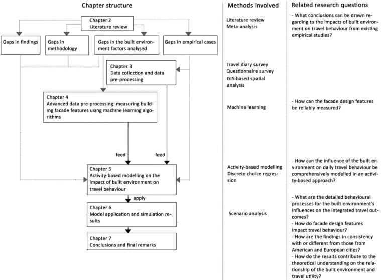
Figure 1-3 Thesis organisation and structure ... 16

Figure 2-1 Subdivision of daily activity-travel behaviour ... 25

Figure 2-2 Gains and costs of travel in relation to travel distance ... 27

Figure 2-3 Net travel utility in relation to travel distance (an example) ... 28

Figure 2-4 Assumed changes in travel gains and costs following enhanced density, diversity and destination accessibility ... 30

Figure 2-5 Assumed changes in travel gains and costs following enhanced road density/connectivity ... 31

Figure 2-6 Assumed changes in travel gains and costs following reduced distance to transit ... 32

Figure 2-7 Assumed changes in travel gains and costs following increased parking space ... 33

Figure 2-8 Assumed changes in travel gains and costs following enhanced street facade design ... 34

Figure 3-1 Base map of Beijing (coloured area indicates the study area) ... 58

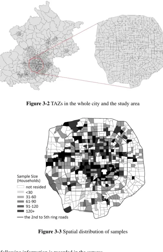
Figure 3-2 TAZs in the whole city and the study area ... 60

Figure 3-3 Spatial distribution of samples ... 60

Figure 3-4 Locations of the selected residences in the small survey ... 64

Figure 3-5 Boundaries of Jiedao and TAZ ... 67

Figure 3-6 Socioeconomic characteristics of the three social groups identified by LCA... 73

Figure 3-7 Population density ... 76

Figure 3-8 Employment density ... 76

(12)

xi

Figure 3-10 Entertainment density ... 77

Figure 3-11 Land use mix ... 78

Figure 3-12 Distance to the city centre ... 80

Figure 3-13 Clustering results using different parameters ... 81

Figure 3-14 Distance to the nearest commercial cluster ... 82

Figure 3-15 Density of primary roads ... 83

Figure 3-16 Density of secondary roads ... 84

Figure 3-17 Density of tertiary roads ... 84

Figure 3-18 Areas of bus coverage using different buffer distances ... 85

Figure 3-19 Bus coverage ... 86

Figure 3-20 Distance to the nearest subway station ... 86

Figure 3-21 Density of parking ... 87

Figure 4-1 Camera facing the street (left) and facing the buildings (right) ... 93

Figure 4-2 Work flow diagram ... 94

Figure 4-3 Rating examples ... 96

Figure 4-4 Comparison between machine scores and expert rating scores on the task of facade quality ... 100

Figure 4-5 Examples of errors in the task of facade continuity ... 101

Figure 4-6 Scores on facade quality ... 102

Figure 4-7 Scores on facade continuity ... 102

Figure 5-1 Model flow diagram ... 113

Figure 5-2 Flow diagram for Sub-model 1 ... 118

Figure 5-3 Flow diagram of Sub-model 2 ... 126

Figure 5-4 Congestion levels by hour ... 134

Figure 5-5 Flow diagram for Sub-model 3 ... 135

Figure 5-6 Flow diagram of Sub-model 4 ... 147

Figure 6-1 Impacts of built environment changes on VMT per capita ... 159

Figure 6-2 Decomposition of the influence of population density ... 161

(13)

xii

Figure 6-4 Decomposition of the influence of retail density ... 162

Figure 6-5 Decomposition of the influence of entertainment density... 162

Figure 6-6 Decomposition of the influence of land use mix ... 163

Figure 6-7 Decomposition of the influence of the distance to commercial clusters ... 164

Figure 6-8 Decomposition of the influence of primary road density ... 165

Figure 6-9 Decomposition of the influence of secondary road density ... 165

Figure 6-10 Decomposition of the influence of tertiary road density ... 165

Figure 6-11 Decomposition of the influence of bus coverage ... 166

Figure 6-12 Decomposition of the influence of bus coverage ... 167

Figure 6-13 Decomposition of the influence of parking density ... 167

Figure 6-14 Decomposition of the influence of facade quality ... 168

Figure 6-15 Decomposition of the influence of facade continuity ... 169

Figure 6-16 Changes in VMT under different regional scenarios... 170

Figure 6-17 Changes in commute VMT under different regional scenarios ... 170

Figure 6-18 Changes in non-commute distance under different regional scenarios ... 172

Figure 6-19 Changes in non-commute VMT under different regional scenarios ... 172

(14)

1

Chapter 01 Introduction

1.1 Motivation and objectives

Transportation is one of the sources of many vexing urban problems, namely, congestion, pollution, inequality and reliance to fossil fuels (Hanson & Giuliano, 2004). Among the many approaches in tackling transport-related problems, a host of urban planning and design philosophies—new urbanism, transit-oriented development, traditional town planning—have gained popularity as ways of shaping travel demand (Cervero & Kockelman, 1997). The theory of consumer choice is used as the theoretical base for the potential influences of the built environment, by assuming that the built environment impacts on (relative) trip costs (Boarnet & Crane, 2001).

Despite of the appealing potential of the built environment in modifying travel behaviour, the true effects need to be materialised with robust empirical evidences. As a consequence, the relationship between the built environment and travel behaviour has been extensively examined and become one of the most heavily researched subjects in urban planning (Ewing & Cervero, 2010). More than two hundred studies have been produced since the 1990s and more are still emerging.

However, existing research tend to focus on the influences of the built environment on the synthesised outcomes of travel (e.g. VMT, walking distance, see the meta-analysis in Section 2.3), while the behavioural processes that give rise to these outcomes have received much less attention. For instance, if a built environment change is found to be related with 10% reduction of VMT, then whether the reduction comes from lower activity frequency, or the choice of closer destinations, or smaller share of driving, or etc. From the practical perspective, different behavioural processes would have

(15)

2 different implications for people’s actual experience and can be related with different policy goals. Besides, gaps also exist in terms of the quite mixed, sometimes contradictory results produced by existing research (Salon, Boarnet, Handy, Spears, & Tal, 2012), as well as the lack of research on fast growing, high density Asian cities (P. Zhao, Lu, & De Roo, 2011) (see the next section for a detailed description of research gaps). Practically, these gaps would also pose challenges to the reliability of the research findings for planning policy making, which is particularly an issue considering that built environment interventions are often costly and long-standing (Cao, 2015a). Therefore, more research efforts are needed in improving the understanding of the relationship between the built environment and travel behaviour from both the theoretical and practical points of view.

The aim of this thesis is thus to explore the influence of the built environment on travel with special emphasis on the behavioural processes and mechanisms. The research will use Beijing as the empirical case. The overarching research question is what impacts the urban built environment has on people’s daily travel behavior. The thesis is guided by the hypothesis that various aspects of daily travel behavior can be influenced by the built environment. More detailed hypotheses in terms of the relationship between different pairs of built environment features and travel outcomes are put forward following a discussion on travel gains and costs in Section 2.1.4.

1.2 Research gaps and related questions

As mentioned before, despite of an overwhelming number of existing research on this topic, there still exist many research gaps. The gaps are related with multiple facets of research, including the methodology adopted, the variables and the cases used and the results. Some of the gaps will be further addressed in the literature review.

(16)

3 The gap in the findings of existing research is twofold. First, as mentioned before, a large proportion of existing findings are about synthesised outcomes of travel, such as VMT, total walking time and so on (see the review by Cervero and Ewing, 2010). It is plausible since these are key indicators of travel behaviour that can be linked with more general policy goals such as energy consumption, emission reduction and public health. However, as explained in the last section, the behavioural processes that give rise to these outcomes and influences have received much less attention (e.g. the travel frequency, destination choice and mode choice that together lead to the outcome of VMT).

Second, there exist a lot of differences in terms of the direction, significance and magnitude of the impacts of the built environment on travel behaviour (see Cervero and Ewing, 2010 for a summary of empirical results produced before 2010 and Appendix A for results produced between 2010 and 2016). It is especially the case in terms of the magnitude of the impacts. For instance, the effect size of the population density in one’s neighbourhood on VMT can range from -0.01 to -0.31, the effect size of land use diversity on VMT can range from -0.10 to -0.36 (these numbers are from only a subset of existing research, see Appendix A). Sources for the differences in findings include the strategies used for data collection, the measurements of built environment features, the statistical models, and more systematically, the varying nature of built environment-travel relationship in different urban contexts. This inconsistency causes a lot vagueness in the understanding on the built environment-travel relationship. Questions remain in terms of to which extent the built environment can direct people towards more sustainable patterns of daily travel, as well as the relative importance of various built environment factors in fulfilling this target (Joh, Nguyen, & Boarnet, 2012; Knuiman et al., 2014).

Gap in methodology

(17)

4 through regressions between synthesised outcomes of travel and a set of socioeconomic and built environment explanatory variables (see Appendix A for a summary of regressions in prior research). The regressions are methodologically sound and robust but when used alone, usually cannot probe into the detailed behavioural processes.

On the other hand, developments in the field of transport simulation and time geography gave rise to the activity-based transport modelling approach. It is underpinned by the notion that travel is derived from the necessity to participate in activities, which in turn reflect needs, desires and commitments of individuals and households, subject to a set of spatial, temporal, institutional, spatial–temporal and possibly budget constraints (Castiglione, Bradley, & Gliebe, 2015; Rasouli & Timmermans, 2014a). Although prototypes began to emerge as early as in the 1970s and substantial progress has been made in developing practical models since the 1990s (Rasouli & Timmermans, 2014a; Yasmin, Morency, & Roorda, 2015), the built environment factors are seldom sufficiently account for in the model systems (see Table 2-5 in Section 2.4 for a summary of built environment variables included in existing activity-based models).

Actually, the activity-based modelling approach can be developed into a helpful tool for the analysis of built environment-travel relationship. The influences of the built environment can be modelled at each detailed choice facet in the activity-travel decision making process (e.g. frequency of activity participation, travel distance for a specific purpose), which will enable a more nuanced understanding on the behavioural mechanisms underlying the observed influences.

Gap in the built environment factors analysed

Built environment factors analysed in existing research are usually sorted as ‘D’ variables, which was first put forward in the seminal work by Cervero and Kockelman (1997) as 3 ‘D’s and then extended to 5 ‘D’s or 6’D’s (Ewing & Cervero, 2001, 2010; Ewing & Handy, 2009). The ‘D’ variables are:

(18)

5 - Density (population density, employment density, building density, etc.)

- Diversity (land use mix, job-housing balance, etc.)

- Design (street density, intersection density, percentage of 4-way/3-way intersection, percentage of cul-de-sac, etc.)

- Destination accessibility (distance to the city centre, distance to ‘regional’ sub-centres, job accessibility by auto/transit in certain time limits, etc.)

- Distance to transit (distance to bus stops, distance to subway stations, etc.) - Demand management (parking supply)

Although these factors already provide a well-rounded account of the built environment, they are mainly two-dimensional and land use-related, while the factors related to the dimension of street facade have received much less attention. These factors can be termed as the seventh ‘D’, the design of street facade. The potential mechanism of the these factors’ influence on travel behaviour can be at least both psychical and functional (Montgomery, 1998; Southworth, 2005). Psychically, some qualities of the facade design may foster positive or negative feelings and thus encourage or discourage physical activities in the urban space (Sarkar et al., 2015; Witten et al., 2012). Functionally, the design and layout may also have an impact on the level of convenience and the utility of travel, e.g. providing much room for street shops at the ground floor. Nonetheless, it should be noted that it is not absolutely rigorous to categorise density and diversity as two-dimensional, since they can also be related to factors like building height or vertical mix.

Gap in empirical cases

By far, most empirical studies on this topic are from American and European (plus a few Oceanian) cities, while evidences from fast growing, high density cities in Asia are relatively scarce (Eom & Cho, 2015; Zegras, 2010; P. Zhao et al., 2011). Such a bias could also undermine the reliability and generalisability of the conclusions made from this line of research, considering that daily travel behaviour involves lots of contextual

(19)

6 specificity (Feng, Dijst, Prillwitz, & Wissink, 2013). Contextual differences that may affect the relationship between built environment and travel behaviour include the level of car ownership, the level of transport service, affordability, social culture, etc. (Feng et al., 2013; Giuliano & Dargay, 2006). Therefore, many studies have argued that scholars should be careful regarding the temporal and spatial transferability of spatial policies (e.g. Badoe and Miller, 1995; Ewing, Tian et al., 2015; Naess, 2015). For example, Ewing, Tian et al. (2015) warned that a study using data from, say, Portland or Houston, can be challenged for relevance to other regions of the US.

A few studies have reported quite different results on the built environment-travel relationship in different countries. For instance, a large number of Asian cities are featured by much higher density comparing with American and European cities (H. Chen, Jia, & Lau, 2008; Madlener & Sunak, 2011). Eom and Cho (2015) found that the impact of high density on reducing car use is greatly reduced when gross density reaches beyond a certain threshold, and some other built environment factors also demonstrate more or less different effects. Giuliano and Dargay (2006) also pointed out that the widespread conviction that higher densities are associated with less travel distance is more pronounced in the US than in Britain. Nonetheless, only very limited research efforts have been made to query the differences in built environment-travel relationship in different urban contexts (e.g. Giuliano and Narayan, 2003; Guiliano and Dargay, 2006; Gim, 2013; Milakis, 2008; Senbil et al., 2009; Feng et al., 2013).

In order to fill in the gaps, the research aims to answer the following questions. (1) To fill the gap in findings - What conclusions can be drawn regarding to the

impacts of built environment on travel behaviour from existing empirical studies? What are the detailed behavioural processes underlying the built environment’s influences on the synthesised travel outcomes? It should be noted that the answer to the second question can also be context dependent, thus it is impossible to reach an ultimate conclusion in one research alone. However, the contribution lies in

(20)

7 raising this issue and proposing a modelling approach to probe into it.

(2) To fill the gap in findings & methodology - How can the influence of the built environment on daily travel behaviour be comprehensively modelled in an activity-based approach?

(3) To fill the gap in the built environment factors analysed – How can the street facade features be reliably measured? How do they impact travel behaviour?

(4) To fill the gap in findings & empirical cases – What are the impacts of the built environment on travel behaviour in Beijing? How are the findings consistent with or different from those from American and European cities? How do the results contribute to the theoretical understanding on the relationship of the built environment and travel utility?

1.3 Choice of the case

The city of Beijing is chosen as the case of study in this research. It is chosen as an example of high-density and fast-growing Asian city, which provides a quite different urban context comparing with American and European cities that have been extensively studied. Since the early 1980s, in parallel with the economic boom, Beijing has been undergoing rapid urban growth. The built-up area increased from 1106.1 square kilometres in 1990 to 2416.5 square kilometres in 2010 and during the same period, the population increased from 5.8 million to 24.2 million. Such growth has made Beijing one of the most-densely resided cities in the world (Figure 1-1).

(21)

8 Figure 1-1 Urban population densities around the world

Note: residents per km2, 2015, screen shot at the same scale

Source: http://luminocity3d.org/WorldPopDen/#9/43.7671/-79.5877

Along with urban growth, the process of motorisation began in Beijing at the end of the 1990s. Between 1999 and 2009, the number of vehicles registered in the city increased rapidly at an annual rate of 17.2%, which was to a large extent contributed by the increase of private cars (P. Zhao & Lu, 2011). During the same period, the total length of roads in Beijing increased from 2,441 to 6,248 kilometres. These trends inevitably changed people’s travel behaviour: the share of driving increased from 5% in 1986 to 32.6% in 2012, and the share of cycling decreased from 62.7% to 13.9% (Beijing Transportation Research Center, 2013). Increasing motorised travel has become a key issue of concern for the sustainable urban development in Beijing: gasoline consumption increased from 26 to 120 toe (the tonne of oil equivalent) per 1000

(22)

9 inhabitants between 1995 and 2004 and road transport accounted for the major share of incremental energy consumption and CO2 emissions (P. Zhao & Lu, 2011). At the same time, urban growth drove more people out of the city centre to former suburban areas, which induced longer commute distances and triggered brisk demand for transportation (Z. Wang, Deng, & Wong, 2016). These conditions will provide a quite different urban context for the analysis of built environment-travel relationship. Besides, for the case itself, it may gain more from such research than the highly urbanised cities since new urban structures, forms and designs are quickly emerging, potentially influencing travel patterns for decades to come (Zegras, 2010).

Figure 1-2 Trends of motorisation in Beijing Source: P. Zhao & Lu, 2011

1.4 General methodology

The over-arching methodology in this thesis is activity-based travel modelling. It simulates activity-travel related decisions such as which activities are conducted when, where, for how long, with whom, and the transport mode involved (Arentze & Timmermans, 2004; Castiglione et al., 2015; Ma, Arentze, & Timmermans, 2012). The strength of the model developed in this research (named as Built Environment Activity-Travel Integrated Model, BEATIM) lies in the comprehensive incorporation of the built

(23)

10 environment conditions in the decision making process. This modelling approach can help address the first and the second gaps in Section 1.2 by linking the activity-based modelling with the built environment-travel analysis and thus enabling a more behavior-oriented and decomposed analysis of the built environment’s influence.

Activity-based models typically fall into one of two paradigms: utility-maximising econometric models and computational process models, though this categorisation is neither exclusive nor exhaustive (Bhat, Guo, Srinivasan, & Sivakumar, 2004; Pinjari & Bhat, 2011; Rasouli & Timmermans, 2014a; Yasmin et al., 2015). Some authors also mentioned a type of constraints-based models, which puts more emphasis on checking whether any given activity agenda is feasible in a specific space–time context (Rasouli & Timmermans, 2014a). The utility-maximising models and the computational process models bear different strengths. The former are more advantageous for the examination of alternative hypotheses regarding the causal relationships between activity-travel patterns, the built environment and socioeconomic characteristics of individuals (Bhat et al., 2004; Yasmin et al., 2015), while the latter are better at modelling decision making under incomplete information and imperfect rationality, and the learning process (Arentze & Timmermans, 2004; Auld & Mohammadian, 2012). The BEATIM model developed in this research generally takes the utility-maximising paradigm for its strength in examining the influences of the built environment, and also incorporates weak computational process features reflected in a series of action rules (see Chapter 5 for detailed description of the model).

Besides, in order to address the third gap, the machine learning method is employed to evaluate the street facade. Usually, this type of built environment features cannot be directly measured from various readily-available geodatabases, but by human field auditors through manual observation and recording (Brownson, Hoehner, Day, Forsyth, & Sallis, 2009). However, the manual nature makes this method inherently expensive and derives few economy of scale (Harvey, 2014). The machine learning method

(24)

11 proposed in this research leverages state-of-the-art techniques and data sources (i.e. online street view images) to realise the automatic evaluation of this type of built environment features (see Chapter 4 for detailed descriptions).

Moreover, several sub-methods are also employed in this research, which include: - Travel diary survey (implemented by the municipal government), on ca. 116,000

individuals, to collect information on people’s 24-h activity-travel behaviour; - Questionnaire survey (implemented by myself), on 200 individuals, to collect

information on people’s travel decision making process;

- GIS-based spatial analysis, on various sources of spatial data, to measure the two-dimensional, land use-related ‘D’ features of the built environment;

- Discrete choice regressions, to estimate the weights of built environment features on various choice facets of activity-travel (activity participation and organisation, location choice for primary destinations and intermediate stops, time of activity and mode choice);

- Scenario analysis, to simulate the impacts of built environment changes on travel behaviour with the proposed activity-based model.

1.5 Research outputs

The main outputs are on three levels:

Theoretical:

Link to the first and second gaps – The research will provide an understanding on the behavioural processes that give rise to the influences of the built environment on daily travel. The results will be examined against the assumptions on the relationship between the built environment and travel (dis)utilities.

(25)

12 of the street facade design on travel behaviour.

Link to the fourth gap – The results from the case study of Beijing, a high density, fast growing Asian city, will be compared with the meta-analysis of the results from American and European cities. Theoretical reflections will be made based on the comparison.

Methodological:

Link to the first and second gaps – The research develops an activity-travel model that comprehensively incorporates the influences of the built environment on various aspects of daily activity-travel.

Policy-related:

Planning policy suggestions for various transport-related goals can be made from the simulation results.

Besides, there are two minor outputs. First, an updated meta-analysis of the effect sizes of built environment features in existing research is provided (see Section 2.3). Second, a machine learning-based method for the automatic evaluation of the street facade design is proposed (see Chapter 4).

1.6 Thesis organisation and structure

After this introduction, Chapter 2 provides a review of the theoretical base and the empirical findings on the built environment-travel relationship, as well as the progresses in activity-based modelling. The theoretical review starts from reviewing the urban planning and design philosophies that advocates the use of the built environment to influence and modify the travel behaviour. The microeconomic theory of utility maximisation is employed to explain the mechanism of this influence, based

(26)

13 on which a series of assumptions on the relationship between various built environment features and travel (dis)utilities are proposed. It is followed by a general review of empirical findings on this topic, and a more quantitative meta-analysis of the effect sizes. Last, the progresses in activity-based modelling are reviewed, with an emphasis on the treatment of built environment features in the existing model systems.

For this chapter, these detailed research questions will be answered:

- What are the theoretical bases for the impact of the built environment on travel behaviour?

- What have existing empirical studies found about the impact of the built environment on travel behaviour? What are the significance levels and magnitudes of the impacts reported by existing studies?

- How are activity-based models constructed?

Chapter 3 introduces the study area, the data sources and the measurement of the built environment features conventionally included in this line of research (the six ‘Ds’). Specifically, the data sources involve two field surveys for the collection of travel-related information, one large travel diary survey on people’s 24h travel behaviour and one small questionnaire survey on the processes of travel decision making.

For this chapter, these detailed research questions will be answered: - What is the spatial extent of the study area

- How are the data for my research collected?

- How are the ‘6D’ features measured from various data sources?

Chapter 4 deals with the measurement of the street facade design, which employs the state-of-the-art machine learning techniques. Two specific features are selected as key factors that could potentially influence the travel behaviour: the construction and maintenance quality of building facade (a building-level feature) and the continuity of

(27)

14 street wall (a street-level feature).

- What features of street facade design can be considered as key factors that could potentially influence the travel behaviour?

- How can street facade features be measured? How is the performance of machine learning algorithms?

Chapter 5 develops the activity-based model, which simulates a sequence of decision making related to daily activity participation and travel, and more importantly, the impacts of the built environment within the process. The design of the model framework, the construction of the four sub-models and the validation results will be discussed in detail.

- How can an activity-based model be designed to effectively simulate the decision making process of daily travel and incorporate the impacts of the built environment? - How can the model parameters be estimated?

- How well can the model perform to approximate the reality?

- In which situations does the model perform well and in which situations does it produce relatively large errors?

Chapter 6 applies the model to simulate the impacts of various built environment changes on travel behaviour through scenario analysis. Two types of scenarios are designed: ‘local’ scenarios, referring to a built environment change in one single TAZ, and ‘regional’ scenarios, referring to the built environment changes in varying buffer zones from a TAZ. As emphasised before, the analysis not only examines the synthesised travel outcomes, but also the behavioural processes. A few policy suggestions are drawn from the simulation results.

(28)

15 For this chapter, these detailed research questions will be answered:

- What are the impacts of various ‘local’ built environment changes on the activity participation and travel behaviour of residents at where the changes take place (e.g. activity frequency, distance of travel, mode choice, etc.)? Specifically, what are the impacts of the two newly-added street facade features?

- What are the impacts of ‘regional’ built environment changes?

- How are the results consistent with or different from those from American and European cities?

- How are the results consistent with or different from theoretical assumptions? What are the implications?

- What are the proper policies for various goals, such as reducing total car use or reducing the travel distance needed for fulfilling daily needs?

In the end, Chapter 7 concludes and discusses the limitations of this research, and points to future directions of research.

(29)

16 Figure 1-3 Thesis organisation and structure

(30)

17

Chapter 02 Literature review

2.1 Theories and assumptions

2.1.1 Philosophies of urban planning and design

It was observed in many cities, especially in the North America, that the increase in car travel has occurred hand in hand with urban sprawl. Consequently, planners plausibly assume that a reversal of this relation by compact urbanisation, densification, and mixed-use development, will reduce the need to travel—particular by car (Maat, Wee, & Stead, 2005). As a result, the idea of using the built environment to influence and modify travel behaviour has found their way into and become one of the key concerns of diverse urban planning and design concepts ever since the early 20th century (Maat et al., 2005; Zegras, 2010). Besides, in the field of transport engineering, the original ‘predictive’ focus of land development-transport analysis evolved to include an increasingly ‘prescriptive’ purpose—i.e. modifying land development patterns explicitly to influence travel demand (Boarnet & Crane, 2001; Zegras, 2010). The key ideas of some of the most influential planning and design strategies that aim at modifying the travel behaviour are briefly reviewed below.

- Jobs-housing balance: advocates that promoting the spatial matches between housing and jobs could help counter the trend of widening separation of suburban workplaces and the residences of suburban workers and increasing peak-period traffic congestion in the US (Cervero, 1989, 1996).

- New Urbanist (or neo-traditional) design: calls for a return to compact neighbourhoods with a combination of neighbourhood design elements including grid-like street patterns, mixed land uses and pedestrian amenities (Lund, 2003; Talen, 2013). It is believed that the neighbourhoods designed in such a manner are

(31)

18 less oriented toward automobile travel and more conducive to walking, bicycling and transit riding, especially for non-commute trips (Cervero & Radisch, 1996; Joh et al., 2012).

- Smart growth: aims to channel new development into existing urban areas and away from undeveloped areas and to improve the viability of alternatives to the car (Handy, Cao, & Mokhtarian, 2005), which are expected to counteract many of the negative effects associated with urban sprawl, including long vehicle travel and congestion (Tracy, Su, Sadek, & Wang, 2011). According to the American Planning Association, compact, transit accessible, pedestrian-oriented, mixed use development patterns and land reuse epitomise the application of the principles of smart growth (American Planning Association, 2002). Actually, there are many overlaps and common technical features between new urbanism and smart growth, as well as other related philosophies such as the walkable city, the compact city and so on (Lund, 2003).

- Compact city: the key idea is to bring activities closer to residents so that they can fulfil their needs and, because the distances are smaller, this allows slower modes (walking and cycling) and public transport to play a bigger role in their travel alternatives and reduces energy consumption and pollution (Aditjandra, Mulley, & Nelson, 2013; Neuman, 2005).

- Walkable city: advocates for better quality of the walking environment in transport planning and design to promote movement by foot and bicycle (Southworth, 2005). It also involves some of the planning and design doctrines mentioned above such as high density, mixed-use, pedestrian-oriented design (further includes high connectivity, safety, high quality of path, etc.), which are supposed to be conducive to walking (Sarkar et al., 2015; Southworth, 2005). Walkability can also be further linked with issues of public health, based on the notion that higher level of physical activity could lead to lower obesity and fewer weight-related chronic conditions, and better overall health (Doyle, KellySchwartz, Schlossberg, & Stockard, 2006). - Transit-oriented development: seeks to maximise access to mass transit and

(32)

non-19 motorised transportation with centrally located rail or bus stations surrounded by relatively high-density commercial and residential developments (Dittmar & Ohland, 2004), which is believed to enhance the attractiveness of public transport services as a whole over the car (Kamruzzaman, Baker, Washington, & Turrell, 2013).

These ideas appear to have made a great impact on modern urban planning and design, both academically and practically (Crane, 1995). Many of the planning and design doctrines have been gradually integrated into the curriculum at the top planning and architecture schools and also incorporated into numerous development plans and projects (Knaap & Talen, 2005). The large influence has naturally given rise to the need for stringent empirical research to testify the promised benefits. As a result, more than two hundred studies have been devoted to analysing the influence of the built environment on travel, particularly the doctrines advocated by the strategies mentioned above. The following sections will provide a review of the relevant research. Section 2.1.2 and 2.1.3 will focus on the theoretical foundation. Section 2.2 to 2.3 will focus on empirical findings.

2.1.2 The built environment, causality and travel

Despite of a large number of studies on examining the assumed influence of the built environment on travel, Naess (2015) critised that “theories explaining why correlations exist between built environment characteristics and travel behaviour are rarely exposed, let alone reflected on”. According to Naess, “compared to the efforts spent on applying the statistical analyses in an as impeccable way as possible, the literature usually spends considerably less space on discussing which variables to include in the statistical models and their order in a causal chain”.

The establishment of a causal relationship is a long standing issue of social research, since many of them seek to determine what causes what in the complex open system of

(33)

20 human society. In fact, the notion of causality itself makes a profound philosophical issue and there is still little agreement on the nature of causation (Beebee, Hitchcock, & Menzies, 2009, p. 1). For instance, some authors think that causation is a relatively non-fundamental feature of the world and can be understood in terms of other more fundamental features such as ‘regularities’; some think that in some sense causation is not a feature of reality at all; others think that causation is about as fundamental as it gets (Beebee et al., 2009, pp. 1-2).

In this thesis, I am not going to dig into the complexity of the philosophical debates on causality, but rather take a more practical framework for the understanding of causation in social research, which is used in the methodological guidebook by Schutt (2011) and Singleton Jr, Straits et al. (1993). According to the framework, there are basically two types of causal explanation in social research, which find their roots in the two intellectual tendencies to knowledge coined by Wilhelm Windelband, termed as nomothetic and idiographic (Schutt, 2011, p. 182). A nomothetic causal explanation identifies common influences on a number of cases or events, which is usually associated with quantitative methods (Schutt, 2011, p. 182). A causal effect from the nomothetic perspective refers to that the variation in one phenomenon leads to or results, on average, in the variation in another phenomenon (Schutt, 2011, p. 182). In contrast, the idiographic causal explanation is more about concrete, individual sequence of events, thoughts, or actions, which can be classified as narrative reasoning and more commonly associated with qualitative methods (Richardson, 1990; Schutt, 2011, p. 184). In the field of built environment-travel research, most existing research are conducted in a quantitative manner and can be considered as reflecting the nomothetic tendency, except for a few works by Naess and collaborators, who consciously took a highly narrative approach from the philosophical position of critical realism (2001, 2015),.

(34)

21 nomothetic causal connection exists, which are: (1) empirical association, (2) appropriate time order (cause precedes effect), (3) non-spuriousness (a relationship between two variables is not due to variation in a third variable), (4) identification of causal mechanism, (5) identification of causal context. While the first criterion is easy to identify with statistical methods, the second and the third requires more sophisticated strategies of research design and data collection. The fourth and the fifth criteria, though not necessarily involve methodological complexity, are much less discussed in existing research.

To be more specific, the time precedence criterion requires approaches that permit multiple directions of causality and/or involve longitudinal measurements. The non-spuriousness criterion needs explicit inclusion of people’s travel attitudes, which is considered to be the major source of spuriousness and the consequence is termed as ‘self-selection’ in this field of research (Cao, Mokhtarian, & Handy, 2009; Mokhtarian & Cao, 2008) (see Cao et al., 2009 for more details in travel attitude-related spuriousness). However, constrained by the costs of data collection, only a small proportion of existing research have, to some extent, incorporated these approaches and more tightly examined the relationship (see Cao et al., 2009 and Mokhtarian et al., 2008 for a review).

The latter two criteria are more about logical deduction for why and under what circumstances the alleged cause should produce the observed effect (Mokhtarian & Cao, 2008). As mentioned at the beginning of this section, Naess (2015) strongly criticised the considerably less research attention on the causal mechanisms. Such a gap may be explained by a general attitude of researchers in this field that takes the existence of a causal mechanism as granted—as Cao et al. (2009) wrote, that “all the statistical methods used in the studies in this field can rely on the travel price changes suggested by Boarnet and Crane (2001) as a plausible causal mechanism”. However, the travel price-based causal mechanism put forward by Boarnet and Crane (2001) is subject to

(35)

22 further refinement in many ways. Therefore, the next section will be spent on reviewing and developing the theoretical explanation for the mechanism of the built environment’s influence on travel behaviour, which, though insufficient alone for the establishment of a causal relationship, could at least help improve the understanding of quantitative results.

2.1.3 Travel as an outcome of utility maximisation

Basically, the aggregate-level relationships between the built environment and travel emerge from a set of transport rationales at the individual-level (Naess, 2015). As mentioned before, most existing works tend to resort to the economic consumer theory that explains individual behaviour and motivations as a result of utility maximisation (Ben-Akiva & Lerman, 1985; Boarnet & Crane, 2001, p. 66; Cervero & Kockelman, 1997; Domencich & McFadden, 1975; Maat et al., 2005; McFadden, 1974; Zegras, 2010). Although the notion of ‘rational man’ and utility maximisation is commonly questioned, the fact that humans are not entirely rational decision-makers with complete information does not imply that they do not at all use instrumental rationality (Naess, 2013). This behavioral paradigm has served as the basis for a rich production of models in transportation-related choice analysis, including the mode of travel, destinations to visit, the household residence, etc. (see examples in Ben-Akiva and Lerman, 1985) (Goulias, 2009). Besides, the repetitive nature of daily travel indicates that people may have already searched and compared many alternatives and optimised their choices from day to day, so that the observed behaviour can be considered as an outcome under near-complete information.

In the framework by Boarnet and Crane (2001), travellers perform trade-offs among available alternatives as in any situation where decisions are made concerning the allocation of scarce resources, whether or not they involve actual money (pp. 61-62). The built environment influences trip-making through impacts on (relative) trip costs (Boarnet & Crane, 2001, pp. 61-62). A later work by Maat et al. (2005) extends this

(36)

23 framework including the benefit side of travel, i.e. activity realisation, following the notion of transport as a derived demand from activity participation, which has an intellectual link with the activity-based approach of travel analysis (Axhausen & Garling, 1992) and Hägerstrand's time geography (1970). The main contribution of Maat et al.’s framework is twofold. First, it assumes that people do notmake separate decisions considering only trips, but that they try to schedule activities in a daily pattern, and therefore, they do not maximise utility for separate travel choices, but optimise their entire activity pattern (Maat et al., 2005). This more integral framework more realistically accounts for the possibility that people may use travel time saved from better accessibility of one activity on participating more other activities (Maat et al., 2005). Second, following the key concept of time geography that both space and time are scarce resources and constrain daily activity patterns (Axhausen & Garling, 1992; Hägerstraand, 1970), the activity-based approach also takes into account the fact that individuals are not free to choose any alternative but are constrained by the total amount of time in a day (Maat et al., 2005).

However, although these frameworks are helpful in understanding the motivations of travel decision making, they do not involve explicit assumptions on the influence of the built environment on travel choices. For instance, Maat et al. (2005) merely briefly discussed the change of the travel utility curve in a condition that is broadly described as ‘compact design’. A related problem is that few published papers in this field ever explicitly stated the hypothesis of research in terms of how travel behaviour would be influenced by built environment (e.g. see Næss, 2013, Cervero & Kockelman, 1997 as examples of those that provided hypothesis) (Naess, 2010). It is especially an issue with the activity-based framework. The assumption of ‘overall utility maximisation’ may lead to more than one mechanism of influence of the causal powers. Some causal mechanisms may amplify each other while others may neutralise or reduce each other’s influences (Naess, 2013). Besides, to the best of my knowledge, none of existing frameworks mentions the gains from travel itself, such as health gains from walking

(37)

24 and cycling, or ‘psychic’ gains from aesthetically pleasing streetscapes (Boarnet & Crane, 2001; Naess, 2013). Therefore, building upon existing works, I would like to put forward a framework which more comprehensively discusses the gains and costs of travel and makes deductions about the influences of the built environment.

Figure 2-1 shows the subdivision of daily activity-travel behaviour based on the activity-based framework, and how they together contribute to the synthesised travel outcomes such as total travel distance and VMT. First, an individual needs to have a general idea about the amount of activity participation in a given day. Activities can be categorised into commute activities (work and go to school), which are usually quite routine and tend to take place at fixed locations, and non-commute activities (all other activities), which are more flexible both in terms of the frequency and the location. For each of the activities that one chooses to participate, a location, a travel mode and a time of activity need to be further selected. These decisions may not have a clear priority and can be mutual influential. For instance, people may perform trip chaining for higher efficiency, in which case multiple activities are combined into one tour so that the total travel distance could be shorter. Besides, considering that people are constrained by the total time budget, the travel costs of one activity (usually more obligatory ones, such as working) can also affect the participation of other activities (usually more discretionary ones). All these subdivided facets together contribute to the synthesised travel outcomes.

(38)

25 Figure 2-1 Subdivision of daily activity-travel behaviour

Maat et al. (2005) analysed the net utility of travel as a function of travel time since they thought that individuals are not primarily interested in travel distance, but rather in the costs of bridging that distance, particularly the time cost. While totally agree with this notion, I still think that it is more appropriate to use travel distance as the independent variable. First, travel distance is more straightforward and predictable given the built environment conditions of an area, while travel time could vary with the traffic speed. Second, travel time is already mediated by the built environment as a function of the travel distance and the road network or the placement of public transit stations, etc., thus it can be considered as a ‘second-order’ variable while travel distance is ‘first-order’.

The diagram in Figure 2-2 illustrates the assumed changes in travel gains and costs as functions of travel distance. As mentioned before, two types of travel gains are considered, gains from conducting activities and gains from travel itself. For non-commute activities, the activity gains generally increase with travel distance since the

(39)

26 further one travels, the more opportunities are within reach and the bigger the chance of being able to reach an opportunity with a higher utility, e.g. cheaper price or more specialised goods (Boarnet & Crane, 2001; Maat et al., 2005). It is assumed that the increase would slow down as the travel distance gets longer, because the additional benefits of travelling longer can be subject to the law of diminishing returns. For example, the second-nearest supermarket might be more attractive than the nearest, perhaps because of lower prices or more variety in products, but the additional benefits of the fifth-nearest compared with the fourth-nearest might be smaller (Maat et al., 2005). It should be noted that, in reality, due to the heterogeneity of the urban space, the curve may not be smooth and continuous but instead bumpy and discontinuous (see Maat et al., 2005 for an example of net travel utility in mixed and concentrated uses). For commute activities, the relationship between travel gains and travel distance can be very bumpy, since the gains can only be realised at places where there are suitable job positions. The more professional and specialised a job is, the more heterogeneous is the distribution of suitable positions.

The travel gains are shown with dotted line since they may not exist if an individual does not value these benefits or does not take a proper travel mode to realise the benefits. For instance, the health benefits of travel are mainly related to active travel modes (walking and cycling) and slightly related to public transit since the trip to and from bus/metro stations may also involve active travel. However they are hardly related to driving or taking taxi. Moreover, these benefits may not even be considered if an individual does not care about health issues. Similarly, the psychic benefits of travelling in an enjoyable urban environment are more experienced if an individual travels in a slow mode and may not actually exist if an individual does not appreciate such qualities. It is assumed that these travel gains are proportional to the travel distance.

The costs of travel are mainly associated with the time spent, the monetary costs and the physical efforts. The curves are differentiated among different travel modes. For

(40)

27 simplicity, three types of modes are considered, which are driving, taking public transit (bus or subway) and active travel (walking or cycling). For driving and taking public transit, the intercepts are above zero since usually some initial actions are required, such as walking to the parking lot, starting the engine, finding a parking space at destination and traveling to and from the subway/bus station, etc. (Maat et al., 2005). Either of the intercepts can be larger than the other, affected by factors such as the distance to public transit stations, the availability of parking spaces, etc. The slope is the highest for active travel since longer time and more physical energy are needed to cover a same distance. Either of the slopes of public transit and driving can be larger than the other, depending on the traffic speed and so on. All curves are supposed to be concave because longer travel could result in growing tiredness, which is the strongest for active travel, medium for taking public transit and the mildest for driving. Another reason for the concave shape is that time is scarce resource so there could be a growing marginal cost. In practice, the shapes of these lines could be more complicatedly affected by the structural conditions of the society, the specific mind set of a person, and the specific conditions of a trip (Naess, 2013). For instance, in a circumstance that drivers are rude and careless, or a person is particularly sensitive to safety risks, the cost slope of active travel could be steeper.

(41)

28 The net utility can then be derived by minusing the costs from the gains as shown in

Figure 2-3. An individual would choose the combination of travel distance and travel mode that produces the highest net utility, if such an alternative is feasible (e.g. not inhibited by car ownership or time budget). It should be noted that, as mentioned before, the shapes of the curves and the positions of the peaks and intercepts may not take the exact form as shown in the figure, but are affected by many factors including the institutional conditions, personal preferences, and more importantly for this research, the built environment settings. In the next part, the impacts of built environment factors on travel gains and costs and the choice outcomes will be discussed.

Figure 2-3 Net travel utility in relation to travel distance (an example)

2.1.4 Assumptions on the influence of the built environment

In travel research, the built environment have often been described through features named with words beginning with D. The ‘three Ds’, coined by Cervero and Kockelman (1997), are density, diversity and (road network) design, followed later by destination accessibility and distance to transit (Ewing & Cervero, 2001; Ewing et al., 2015). Parking supply is also sometimes coined as the sixth ‘D’, namely demand management (Ewing & Cervero, 2010). Besides, as mentioned in the introduction, in order to fill in the gap that the influence of street facade features is seldom analysed (see Section 1.2),

Understanding the impact of built environment on travel behaviour with activity-based modelling: Evidence from Beijing