`
0
-Motivated Low-Rank Sparse Subspace Clustering
Maria Brbi´c and Ivica Kopriva,
Senior Member, IEEE
Abstract—In many applications, high-dimensional data points can be well represented by low-dimensional subspaces. To identify the subspaces, it is important to capture a global and local structure of the data which is achieved by imposing low-rank and sparseness constraints on the data representation matrix. In low-rank sparse subspace clustering (LRSSC), nuclear and
`1 norms are used to measure rank and sparsity. However, the
use of nuclear and `1 norms leads to an overpenalized problem
and only approximates the original problem. In this paper, we propose two`0quasi-norm based regularizations. First, the paper presents regularization based on multivariate generalization of minimax-concave penalty (GMC-LRSSC), which contains the global minimizers of `0 quasi-norm regularized objective. Af-terward, we introduce the Schatten-0 (S0) and `0 regularized objective and approximate the proximal map of the joint solution using a proximal average method (S0/`0-LRSSC). The resulting
nonconvex optimization problems are solved using alternating direction method of multipliers with established convergence conditions of both algorithms. Results obtained on synthetic and four real-world datasets show the effectiveness of GMC-LRSSC andS0/`0-LRSSC when compared to state-of-the-art methods.
Index Terms—alternating direction method of multipliers, gmc penalty,`0regularization, low-rank, sparsity, subspace clustering
I. INTRODUCTION
H
IGH dimensional data analysis is a widespread problem in many applications of machine learning, computer vision, and bioinformatics [1]–[6]. However, in many real-world datasets, the intrinsic dimension of high-dimensional data is much smaller than the dimension of the ambient space and data can be well represented as lying close to a union of low-dimensional subspaces. The problem of segmenting data according to the low-dimensional subspaces they are drawn from is known as subspace clustering [7]. Thanks to their capability to handle arbitrarily shaped clusters and their well-defined mathematical principles, spectral based methods [8], [9] are widely used approaches to subspace clustering. These methods solve the subspace clustering problem by relying on the spectral graph theory and cluster eigenvectors of the graph Laplacian matrix corresponding to the smallest eigenvalues [10].One of the main challenges in subspace clustering is the construction of the affinity matrix that captures well
This work was supported by the Croatian Science Foundation grant IP-2016-06-5235 (Structured Decompositions of Empirical Data for Computationally-Assisted Diagnoses of Disease) and by the European Re-gional Development Fund under the grant KK.01.1.1.01.0009 (DATACROSS). M. Brbi´c and I. Kopriva are with the Laboratory for Machine Learning and Knowledge Representation, Division of Electronics, Rudjer Boskovic Institute (e-mail: [email protected]; [email protected]).
(di)similarities between data points. Among various ap-proaches proposed in the literature, methods based on sparse [11], [12] and low-rank representations [13]–[15] have been among the most successful in many applications [16]. These methods exploit the self-expressiveness property of the data and represent each data point as a linear combination of other data points in the dataset. Low-rank representation (LRR) [13], [14], [17] captures the global structure of the data by imposing a low-rank constraint on the data representation matrix. Low-rank implies that representation matrix is described by a weighted sum of small number of outer products of left and right singular vectors. In order to ensure convexity of the related optimization problem, the rank minimization is relaxed as the nuclear or Schatten-1 norm minimization problem [18]– [20]. Different from LRR, Sparse Subspace Clustering (SSC) [11], [21] captures local linear relationships by constraining representation matrix to be sparse. Using the tightest convex relaxation of the`0 quasi-norm, the SSC model solves sparsity maximization problem as`1 norm minimization problem [22], [23]. Both LRR and SSC guarantee exact clustering when subspaces are independent, but the independence assumption is overly restrictive for many real-world datasets [24], [25]. Under appropriate conditions [26], SSC also succeeds for disjoint subspaces. However, when the number of dimensions is higher than three, SSC can face connectivity problems resulting in a disconnected graph within a subspace [27]. A natural way to construct adaptive model able to capture the global and the local structure of the data is to constrain representation matrix to be low-rank and sparse. In [16], [28]– [30] that is done by combining nuclear and`1 norms as the measures of rank and sparsity, respectively. The motivation lies in the fact that minimization of these norms results in a convex optimization problem.
Although convex, nuclear and `1 norms are not exact measures of rank and sparsity. Therefore, optimal solution of the nuclear and `1 norms regularized objective is only approximate solution of the original problem [31]. Proxim-ity operator associated with the nuclear norm overpenalizes large singular values, leading to biased results in low-rank constrained optimization problems [32], [33]. Similarly, in sparsity regularized problems`1 norm solution systematically underestimates high amplitude components of sparse vectors [34]. Nonconvex regularizations based on `p quasi-norms
(0 ≤ p <1) or their approximations have been proposed for various low-rank [32], [33], [35]–[39] and sparsity regularized problems [34], [40]–[47]. Recently, nonconvex approximations of rank and sparsity have also been introduced in subspace clustering problem [48]–[52]. Specifically, `0-induced sparse subspace clustering is introduced in [48]. The correspond-ing optimization problem is solved uscorrespond-ing proximal gradient descent which under assumptions on the sparse eigenvalues
978-1-5386-5541-2/18/$31.00 c2018 IEEE.
converges to a critical point. In [49] authors replaced the nuclear norm regularizer with the nonconvex Ky Fan p
-k norm [53] and proposed proximal iteratively reweighted optimization algorithm to solve the problem. In [50], [54] rank is approximated using Schatten-q quasi-norm regularization (0 < q < 1). The optimization problem in [50] is solved using generalized matrix soft thresholding algorithm [55]. Schatten-q quasi-norm minimization with tractable q = 2/3 and q =1/2 is proposed in [51]. The Schatten-q (Sq)
quasi-norm for 0 < q < 1 is equivalent to `q quasi-norm on
vector of singular values. Compared to the nuclear norm, it makes a closer approximation of the rank function. In this regard, S0 quasi-norm can be seen as an equivalent to the `0 quasi-norm and stands for the definition of the rank function. Furthermore, [52] combines Sq regularizer (0 < q < 1) for
low-rank and `p quasi-norm regularizer (0 < p < 1) for
sparsity constraint. However, recent results in [56] show that in`p regularized least squares (0≤p<1) smaller values of p
lead to more accurate solutions. If`1 norm is also considered, authors show that for large measurement noises`1outperforms
`p, p <1. However, for small measurement noises `0 quasi-norm regularization outperforms`p,0<p≤1.
Motivated by the limitations discussed above, we intro-duce two S0/`0 quasi-norm based nonconvex regularizations for low-rank sparse subspace clustering (LRSSC). First, we propose regularization based on multivariate generalization of the minimax-concave penalty function (GMC), introduced in [34] for sparsity regularized linear least squares. Here, this approach is extended to the rank approximation. The GMC penalty enables to maintain the convexity of low-rank and sparsity constrained subproblems, while achieving better approximation of rank and sparsity than nuclear and
`1 norms. Importantly, this regularization is closely related to the continuous exact `0 penalty which contains the global minimizers of `0 quasi-norm regularized least-squares objec-tive [34], [57]. GMC penalty yields solutions of low-rank and sparsity constrained subproblems based on firm thresholding of singular values and coefficients of representation matrix, respectively. The firm thresholding function Θ:R→Ris is
defined as [58]: Θ(x;λ,a)= 0, if |x| ≤λ
a(|x| −λ)/(a−λ)sign(x), ifλ≤ |x| ≤a
x, if |x| ≥a.
(1)
Next, we propose the direct solution of S0 and `0 quasi-norms regularized objective function. The solution of corre-sponding low-rank and sparsity constrained subproblems is based on iterative application of hard thresholding operator [59]–[61] on the singular values and coefficients of the repre-sentation matrix, respectively. The hard thresholding function
H:R→R is defined as [59]: H(x;λ)= x, if|x|>√2λ {0,x}, if|x|=√2λ 0, if|x|<√2λ. (2) Simultaneous rank and sparsity regularization is handled using the proximal average method, introduced in [62] for convex
problems and extended recently to nonconvex and nonsmooth functions [63], [64]. Proximal average allows us to approxi-mate the proximal map of joint solution by averaging solutions obtained separately from low-rank and sparsity subproblems, leading to a problem with a low computational cost in each iteration. Furthermore, using proximal average method enables us to establish global convergence guarantee for S0/`0 regu-larized LRSSC.
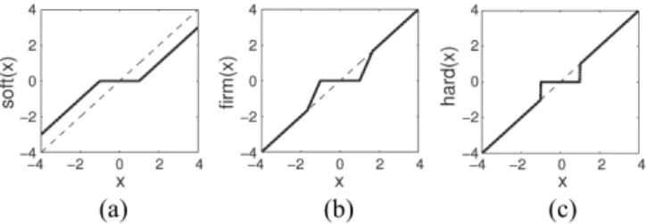
Better approximation of rank and sparsity is a consequence of the properties of firm and hard thresholding operators asso-ciated with GMC and`0 regularizations. As opposed to them, the soft thresholding operator underestimates high amplitude coefficients in `1 norm based sparsity regularized objective, as well as large singular values in low-rank approximation problem. As an example, Fig. 1 shows soft, firm and hard thresholding operators used in LRSSC, GMC-LRSSC and
S0/`0-LRSSC, respectively.
Fig. 1. Proximity operators for threshold valueλ=1. (a) Soft-thresholding operatorso f t(x;λ)=sign(x)max(0,|x| −λ)is associated with`1norm.
(b) Firm-thresholding operator defined in (1) and associated with the scaled MC penalty and used in GMC-LRSSC formulation. Parameter a is for visualization proposes set to0.6. (c) Hard-thresholding operator defined in (2) and associated with`0quasi-norm.
To solve corresponding optimization problems we derive algorithms based on computationally efficient Alternating Direction Method of Multipliers (ADMM) [65]. Although ADMM has been successfully applied for many nonconvex problems [66]–[68], only recent theoretical results establish convergence of ADMM for certain nonconvex functions [69]– [72]. For GMC regularization, we show that the sequence generated by the algorithm is bounded and prove that any limit point of the iteration sequence is a stationary point. For
S0/`0regularization with proximal average approach, based on the property that `0 andS0 quasi-norms belong to a class of semialgebraic functions and satisfy the Kurdyka-Łojasiewicz inequality [73], the global convergence of the algorithm can be guaranteed.
Experimental results on synthetic and four real-world datasets demonstrate that the proposed `0 based low-rank sparse subspace clustering algorithms converge fast and to a point with lower or similar clustering error than the convex approximations with nuclear and `1 norms. Compared to the state-of-the-art subspace clustering methods, the proposed algorithms perform better on four benchmark datasets.
A. Contributions
The contributions of this paper are summarized as follows: 1) We introduce nonconvex generalized minimax-concave penalty in the low-rank sparse subspace clustering
prob-lem, such that the global minimizers of the proposed objective coincide with that of a convex function defined using the continuous exact `0 penalty [57]. The intro-duced penalty maintains the convexity of the sparsity and low-rank constrained subproblems. The proximal operator of the related GMC penalty function is the firm thresholding function [34].
2) We introduceS0 and`0 pseudo-norm regularizations for LRSSC. Using the proximal average method [62], [63], we average the solutions of proximal maps of low-rank and sparsity subproblems, with the hard thresholding function as a proximity operator of the related penalties [59].
3) We derive ADMM based optimization algorithms for LRSSC constrained either with a GMC penalty or with
S0/`0 quasi-norms. Iterative firm or hard thresholding of singular values and coefficients of representation matrix is used to obtain the solution of rank and sparsity constrained subproblems.
4) We prove that the sequence generated by the GMC regularized LRSSC algorithm is bounded and that any limit point of the iteration sequence is a stationary point that satisfies Karush-Kuhn-Tucker (KKT) conditions. 5) We establish the convergence property of the S0/`0
reg-ularized approach with proximal average and show that the algorithm converges regardless of the initialization. To the best of our knowledge, we are the first to show convergence with S0 and `0 penalties in the low-rank and sparsity constrained optimization problem.
The remainder of this paper is organized as follows. Section II gives a brief overview of the related work. In Section III and IV we introduce GMC and S0/`0 regularized low-rank sparse subspace clustering methods, respectively. We formu-late the problem, present optimization algorithms, and analyze convergence and computational complexity. The experimental results on synthetic and four real-world datasets are presented in Section V. Finally, Section VI concludes this paper.
B. Main Notation
Scalars are denoted by lower case letters, vectors by bold lower-case letters, matrices are denoted by bold capital and subspaces by calligraphic letters.k ·kFdenotes Frobenius norm
defined as the square root of the sum of the squares of matrix elements.k · k1 denotes`1 norm defined as the sum of absolute values of matrix elements. k · k∗denotes nuclear norm defined as the sum of singular values of a matrix. `0 quasi-norm is denoted by k · k0 and for matrix A∈RN×M defined as:
kAk0 =#ai j ,0, i=1..N, j=1..M ,
where # denotes cardinality function. Schatten-0 quasi norm is denoted by k · kS0 and defined as:
kAkS0 =kdiag(Σ)k0,
where A = UΣVT is the singular value decomposition (SVD) of matrix A. Since `0 quasi-norm does not satisfy homogeneous property it is not a norm, but with a slight abuse of notation we will refer to it as the`0 norm in the rest of the
paper. Null vector is denoted by 0 and diag(·) is the vector of diagonal elements of a matrix. Table I summarizes some notations used in the paper.
TABLE I
NOTATIONS AND ABBREVIATIONS Notation Definition
N Number of data points
n Dimension of data points
L Number of subspaces
X∈Rn×N Data matrix
C∈RN×N Representation matrix
W ∈RN×N Affinity matrix
X=UΣVT Singular value decomposition ofX
σ(X) Vector of singular values ofX
II. BACKGROUND
Consider the data matrix X ∈Rn×N the columns of which
are data points drawn from a union of L linear subspaces
ÐL i=1Si of unknown dimensions di =dim(Si) iL=1 inRn. Let Xi ∈ Rn×Ni be a submatrix of X of rank d i, 0 < di < Ni and ÍL
i=1Ni = N. Given data matrix X, subspace clustering
segments data points according to the low-dimensional sub-spaces. The first step is the construction of the affinity matrix W ∈RN×N whose elements represent the similarity between
data points. An ideal affinity matrix is block diagonal (up to a permutation): non-zero distance is assigned to the points in the same subspace and zero distance to the points from different subspaces. Spectral clustering algorithm [8], [9] is then applied to the affinity matrix to obtain memberships of data points to the subspaces.
A. Related Work
Low-Rank Representation (LRR) [13], [14] aims to find a low-rank representation matrixC ∈RN×N for input data
ma-trixX by solving the following convex optimization problem: min C C ∗ s.t. X=X C, (3)
where the nuclear norm is used to approximate the rank ofC. Let X =UΣVT be the SVD of X. The closed form solution
of problem (3) is given by [14]: ˆ
C=V VT. (4)
When data points are contaminated by additive white Gaus-sian noise (AWGN), the following minimization problem is solved: min C λ 2 X−X C 2 F+ C ∗, (5)
where λ is the rank regularization constant. The optimal solution of problem (5) is given by [17], [74]:
ˆ C=V1(I− 1 λΣ−21 )V T 1, (6) where U = [U1 U2], Σ = diag(Σ1 Σ2) and V = [V1 V2]. Matrices are partitioned according to the setsI1 ={i :σi >
1 √
λ} and I2 = {i : σi ≤
1 √
λ}, where σi denotesith singular
value of X.
Sparse Subspace Clustering (SSC) [11] represents each data point as a sparse linear combination of other data points and solves the following convex optimization problem:
min C C 1 s.t. X =X C, diag(C)=0, (7)
where constraintdiag(C)=0 is used to avoid trivial solution of representing a data point as a linear combination of itself. For data contaminated by the AWGN, the following mini-mization problem is solved to approximate sparse representa-tion matrixC: min C 1 2 X−X C 2 F+τ C 1 s.t. diag(C)=0, (8) where τ is the sparsity regularization constant. This problem can be solved efficiently using ADMM optimization procedure [11], [65].
Low-Rank Sparse Subspace Clustering (LRSSC) [29] re-quires that the representation matrix Cis simultaneously low-rank and sparse. LRSSC solves the following problem:
min C λ C ∗+τ C 1 s.t. X =X C, diag(C)=0, (9) whereλ andτ are rank and sparsity regularization constants, respectively. For the AWGN corrupted data the following problem needs to be solved to approximate C:
min C 1 2 X−X C 2 F+λ C ∗+τ C 1 s.t. diag(C)=0. (10) After representation matrix C is estimated, the affinity matrix W ∈RN×N is calculated as follows:
W =|C|+|C|T. (11) In the next two sections, we introduce two nonconvex regularizers for the low-rank sparse subspace clustering. We formulate low-rank sparse subspace clustering problem in the following general form:
min C 1 2 X−X C 2 F+λg(C)+τf(C) s.t. diag(C)=0, (12) whereg(C)and f(C)are functions that, respectively, measure rank and sparsity of the data representation matrix C. The convex formulation used in (10) implies g(C) = C
∗ and f(C)=C 1. III. GMC-LRSSC ALGORITHM A. Problem Formulation
We propose to regularize rank and sparsity using multi-variate GMC penalty function, introduced in [34] for sparse regularized least-squares. We start with some definitions and results that will be used throughout the paper.
Definition 1 ( [34]):Letz∈RN andB∈
RM×N. The GMC
penalty function ψB:RN →Ris defined as:
ψB(z)=kzk1−SB(z), (13)
whereSB:RN →Ris the generalized Huber function defined
as: SB(z)= inf v∈RN n kvk1+1 2kB(z−v)k 2 2 o . (14) Lemma 1 ( [34]): Let z ∈ RN, y ∈ RM, A ∈ RM×N and λ >0. Define F:RN →Ras: F(z)=1 2ky−Azk 2 2 +λψB(z), (15) where ψB : RN → R is the GMC penalty. If ATA−λBTB
is positive semidefinite matrix, F is a convex function. The convexity condition is satisfied by setting:
B=pγ/λA, 0≤γ≤1. (16) The parameter γ controls the nonconvexity of the penalty
ψB. Larger values of γ increase the nonconvexity of the penalty.`1 norm can be seen as a special case of this penalty by settingγ=0.
Lemma 2 ( [34]): Let z ∈ RN, y ∈ RM, A ∈ RM×N and
λ >0. If ATAis diagonal with positive entries andBis given by (16), then for 0 < γ ≤1 the minimizer of F is given by element-wise firm thresholding. Formally, if
ATA=diag(α21, ..., α2N), (17) then
zoptn =Θ([ATy]n/α2n;λ/α2n, λ/(γα2n)), (18)
whereΘstands for the firm thresholding function [58] defined entry-wise in (1).
Definition 2 ( [75], [76]): Function f : RN → R is an
absolutely symmetric function, if:
f(z1,z2, ...,zN)= f(|zπ(1)|,|zπ(2)|, ...,|zπ(N)|), (19) holds for any permutation πof {1, ...,N}.
Proposition 1: Let BTB be a diagonal matrix and ψ
B be the GMC penalty function defined in (13). The subdifferential of singular value function ψB◦σ of a matrix X is given by the following equation:
∂[(ψB◦σ)(X)]=Udiag(∂ψB[σi(X)])VT, (20)
where X=UΣVT is the SVD of X.
Proof: It follows from [34] that ifBTBis a diagonal matrix, the GMC penaltyψB is separable, comprising a sum of scalar MC penalties: BTB=diag(α12, ..., αN2) ⇒ψB(z)= N Õ n=1 φαn(zn), (21) whereφb:R→Ris the scaled MC penalty [34], [77] defined
as: φb(y)= ( |y| −12b2y2, if |y| ≤1/b2, 1 2b2, otherwise. (22) Therefore, according to Definition 2, ψB is an absolutely symmetric function. The proof of the proposition then follows from the property of the singular value function f ◦σ [76], where f is an absolutely symmetric function.
Proposition 1 allows us to use GMC penalty for rank ap-proximation. We formulate GMC penalty regularized objective
for low-rank sparse subspace clustering. Let B∈RN×N, and
let σ(C) denote vector of singular values ofC. By choosing
g(C)=ψB(σ(C)) as a rank function, and f(C) =ψB(C) as a sparsity function in equation (12), we define the following nonconvex objective function:
min C 1 2 X−X C 2 F+λψB(σ(C))+τψB(C) s.t. diag(C)=0, (23) where ψB denotes GMC penalty defined in (13), regularized by matrixB. In the next section we will show that by solving the objective (23) with ADMM, both sparsity and low-rank subproblems can be reduced to the equation (15) with diagonal ATA. In this case, GMC penalty is closely related to the continuous exact `0 penalty [34], [57], that approximates the convex hull of the least squares with`0regularization. Further-more, diagonal ATA reduces both subproblems to
element-wise firm thresholding function, defined in (1). In low-rank minimization subproblem, the firm thresholding operator needs to be applied to the vector of singular values.
B. Optimization Algorithm
To solve optimization problem in (23), we introduce aux-iliary variables J, C1 and C2 to split variables and solve subproblems independently. The reformulated objective for GMC penalty in (23) is equivalent to:
min J,C1,C2 1 2 X−X J 2 F+λψB(σ(C1))+τψB(C2) s.t. J =C1, J =C2−diag(C2), (24) The augmented Lagrangian function of (24) is:
Lµ1,µ2 J,C1,C2,Λ1,Λ2= 1 2 X−X J 2 F+λψB(σ(C1)) +τψB(C2)+ µ1 2 J−C1 2 F+ µ2 2 J−C2+diag(C2) 2 F + Λ1,J−C1 + Λ2,J−C2+diag(C2) , (25) where µ1, µ2 > 0 are penalty parameters and Λ1, Λ2 are Lagrange multipliers.
Update rule for Jk+1: Given Ck
1, C k 2,Λ k 1, Λ k 2, µk1, µ k 2, we minimize the Lagrangian function in (25) with respect to J:
min J Lµ1k,µ k 2 C k 1,C2k,J,Λk1,Λk2 = min J 1 2 X−X J 2 F +µ1 2 J−C1k 2 F+ µ2 2 J−C2k+diag(C2k) 2 F+ Λk1,J−C1k + Λk2,J−C2k+diag(C2k). (26) The optimal solution of (26) is given by the following update: Jk+1 =XTX+(µk1+µk2)I−1XTX+µk1C1k+µ2kC2k−Λ1k−Λ2k
.
(27)
Update rule for Ck+1
1 :Given J
k+1,Λk
1, µk1, we minimize the
Lagrangian function in (25) with respect to C1: min C1 Lµk 1,µ k 2 J k+1,C 1,C2k,Λk1,Λ2k =min C1 λψB(σ(C1))+ µk 1 2 Jk+1−C1 2 F+ Λk1,Jk+1−C1 =min C1 λψB(σ(C1))+ µk 1 2 J k+1+Λ k 1 µk 1 −C1 2 F. (28) It can be seen that (28) corresponds to the least squares problem in (15) with ATA = I and therefore, diagonal. It
follows from the condition (16) that in order to maintain convexity of the subproblem, we need to set B=
q
µk
1γ/λI, 0 < γ ≤ 1. Using Lemma 2 and Proposition 1, (28) can be solved by element-wise firm thresholding of singular values of matrix Jk+1+Λk1/µk1
.
Specifically, letUΣVT denote the SVD of matrix Jk+1+
Λ1k/µk1. The closed-form solution of (28) is given by: C1k+1 =UΘ Σ; λ µk 1 , λ γµk 1 VT, (29) whereΘis the firm thresholding function defined in (1).
Update rule for C2k+1: Given Jk+1, Λk2, µk2, we minimize the objective (25) with respect to C2:
min C2 Lµk 1,µ k 2 J k+1,Ck+1 1 ,C2,Λk1,Λk2 =min C2 τψB(C2)+ µk 2 2 J k+1+Λ k 2 µk 2 −C2 2 F, (30)
with subtraction of diagonal elements ofC2k+1:
C2k+1←C2k+1−diag C2k+1. (31) Similarly as the update forC1, matrixATAis diagonal matrix and we can ensure convexity of the subproblem (30) by setting B=qµk
2γ/τI, 0 < γ ≤1. The problem (30) is then solved by firm thresholding elements of matrix Jk+1+Λk2/µk2
and given by: C2k+1 =Θ Jk+1+Λ k 2 µk 2 ; τ µk 2 , τ γµk 2 , C2k+1←C2k+1−diag C2k+1. (32)
Update rules for Lagrange multipliersΛt1+1,Λ2t+1:GivenJk+1, C1k+1,C2k+1,µk1,µk2, Lagrange multipliers are updated with the following equations:
Λk1+1 =Λk1 +µ1k Jk+1−C1k+1
Λk2+1 =Λk2 +µk2 Jk+1−C2k+1. (33)
Penalty parameters µ1, µ2 are are in each step k updated according to:
µik+1=min(ρµik, µmax), i=1,2, (34)
where ρ >1 is step size for adaptively changing µ1, µ2. Due to numerical reasons µ1, µ2 are bounded with µmax, while in the convergence proof we use formulation µik+1 = ρµik, i=1,2.
The main steps of the proposed algorithm are summarized in Algorithm 1.
Algorithm 1 GMC-LRSSC by ADMM optimization
Input: Data points as columns in X ,{τ, λ}>0,0< γ≤1
Output: Assignment of the data points to kclusters
1: Initialize: J,C1,C2,Λ1,Λ2 =0,{µ(0)i >0}i2=1, ρ >1
2: Compute XTX for later use 3: whilenot converged do 4: Update Jk+1 by (27)
5: Normalize columns of J to unit`2 norm
6: UpdateCk+1
1 by (29)
7: UpdateCk+1
2 by (32)
8: UpdateΛk1+1,Λk2+1 by (33)
9: Update µki+1 =min(ρµki, µmax),i=1,2
10: end while
11: Calculate affinity matrixW =|C1|+|C1|T
12: Apply spectral clustering [9] toW
C. Convergence Analysis
Although choosing γ ∈ [0,1] guarantees convexity of the low-rank and sparsity subproblems and convergence of related subproblems, the objective in (23) is nonconvex. In this section, we analyze convergence of the proposed method and show that any limit point of iteration sequence satisfies Karush-Kuhn-Tucker (KKT) conditions [78].
Proposition 2:The sequences(Jk,C1k,C2k,Λk1,Λk2) gener-ated by Algorithm 1 are all bounded.
We now state the main theorem related to convergence property of GMC-LRSSC algorithm.
Theorem 1: Let Yk = Jk,C1k,C2k,Λk1,Λk2 ∞
k=1 be a sequence generated by Algorithm 1. Suppose that limk→∞ Yk+1 −Yk = 0. Then, any accumulation point of the sequence {Yk ∞
k=1 satisfies the Karush-Kuhn-Tucker (KKT) conditions for problem (24). In particular, whenever
{Yk ∞k=1 converges, it converges to a point that satisfies KKT conditions.
The proofs of Proposition 2 and Theorem 1 are given in the Appendix.
D. Stopping Criteria and Computational Complexity
The steps in Algorithm 1 are repeated until convergence or until the maximum number of iterations is exceeded. We check the convergence by verifying the following inequalities at each iteration k:Jk −Ck 1k∞ ≤, Jk−Ck 2k∞ ≤, Jk − Jk−1k
∞ ≤. We found that setting error tolerance to=10−4 works well in practice. In each step we normalize columns of matrixJ. This normalization is frequently applied to stabilize convergence of non-negative matrix factorization algorithms [79].
The computational complexity of Algorithm 1 is O(nN2+ T N3), where T denotes the number of iterations. In the experiments, we set the maximalT to100, but on all datasets the algorithm converged within less than 15 iterations. Note that the computational complexity of spectral clustering step isO(N3).
IV. S0/`0-LRSSC ALGORITHM A. Problem Formulation
In addition to the GMC penalty, we propose to directly use
S0 and`0 as constrains for low-rank and sparsity. Specifically, by choosing g(C) = kCkS0 as a rank function, and f(C) =
kCk0 as a measure of sparsity in formulation (12), we obtain the following nonconvex optimization problem:
min C 1 2 X−X C 2 F+λ C S0+τ C 0 s.t. diag(C)=0. (35) The proximity operator H:R→R of kxk0 is defined entry-wise as: H(y;λ)=argmin x∈R n1 2(y−x) 2+λkxk 0 o , (36)
The closed form solution of (36) at y ∈ R is the hard thresholding function defined in (2). The proximity operator of C
S
0 is the hard thresholding function applied entry-wise to the vector of singular values [60], [61].
B. Optimization Algorithm
To solve minimization problem in (35), we split original problem into two variables J and C. That leads to the following objective function:
min J,C 1 2 X−X J 2 F+λkCkS0+τkCk0 s.t. J =C−diag(C), (37) The augmented Lagrangian function of (37) is:
Lµ J,C,Λ = 1 2 X−X J 2 F+λkCkS0+τkCk0 +µ 2 J−C+diag(C) 2 F+ Λ,J−C+diag(C), (38) where µis penalty parameter andΛis Lagrange multiplier.
Update rule for Jk+1: Given Ck, Λk, µk, minimization of
the Lagrangian function in (38) yields the following update: Jk+1=XTX+µkI−1XTX+µkCk−Λk. (39)
Update rule for Ck+1: Given Jk+1, Λk, µk, the following
problem needs to be solved: min C λ C S0+τ C 0+ µk 2 J k+1+Λk µk −C 2 F. (40)
Whenλ,0 andτ=0, the proximal map reduces to:
Pgµ =arg min C λ C S0+ µk 2 J k+1+Λk µk −C 2 F. (41)
Let UΣVT denote the SVD of matrix Jk+1 +Λk/µk
. The closed-form solution of (41) is given by:
Ck+1=UH Σ; λ µk VT, (42)
whereH is the hard thresholding function defined in (2) and applied entry-wise toΣ. Similarly, when λ=0andτ,0the
proximal map is given by: Pµf =arg min C τ C 0+ µk 2 J k+1+Λk µk −C 2 F. (43)
Closed-form solution of (43) is obtained by the hard threshold-ing operator H applied entry-wise to matrix Jk+1+Λk/µk
: Ck+1=HJk+1+Λ k µk; τ µk , Ck+1←Ck+1−diag Ck+1. (44) Proximal average, introduced recently in [62] and general-ized to nonconvex and nonsmooth setting in [63], [64], allows us to efficiently solve problem in (40) whenλ,0 andτ,0. In particular, given that the proximal maps Pµf and Pgµ can be easily solved using the hard thresholding operator, we approximate the proximal map Pµf+g by averaging solutions of proximal maps of low-rank and sparse regularizers:
Pµf+g ≈λPgµ+τPµ
f, (45)
where parameters τ andλare set such that τ+λ=1. Furthermore, since `0 and S0 norms belong to the class of semi-algebraic functions [73], the proximal average function
Pf+g is also a semi-algebraic function [63].
Update rule for Lagrange multiplier Λt+1: Given Jk+1, Ck+1, µk, Lagrange multiplier is updated with the following
equation:
Λk+1=Λk+µk Jk+1−Ck+1
(46) The main steps of the proposed algorithm are summarized in Algorithm 2.
Algorithm 2 S0/`0-LRSSC by ADMM optimization
Input: Data points as columns in X ,{τ, λ}>0,τ+λ=1
Output: Assignment of the data points to kclusters
1: Initialize: J,C,Λ =0, µ(0)>0,ρ >1
2: Compute XTX for later use 3: whilenot converged do 4: Update Jk+1 by (39)
5: Normalize columns of J to unit`2 norm
6: Calculate rank regularized proximal mapPgµ by (42)
7: Calculate sparsity regularized proximal mapPµf by (44)
8: UpdateCk+1=Pµf+g defined in (45), (41), (43)
9: UpdateΛk+1 by (46)
10: Update µk+1 =min(ρµk, µmax) 11: end while
12: Calculate affinity matrixW =|C1|+|C1|T
13: Apply spectral clustering [9] toW
C. Convergence Analysis
Theorem 2: Let Yk = Jk,Ck,Λk ∞
k=1 be a sequence generated by Algorithm 2. Then, for any sufficiently large µ, Algorithm 2 converges globally1.
1That is, regardless of the initialization, it generates a bounded sequence
that has at least one limit point which is a stationary point of (38).
Proof: The results in [63] guarantee convergence of the proximal average method. To guarantee global convergence of the Algorithm 2, we rewrite the problem (37) using the following more general form:
min C,J f1(C)+f2(J) subject to AC=BJ, (47) where A = I, B = I, f1(C) = λkCkS0 +τkCk0, f2(J) = 1 2 X−X J 2 F.
We will now show that the assumptions A1-A5 in [70] which guarantee convergence in nonconvex nonsmooth op-timization problem are satisfied. k · k0 and k · kS0 are non-negative lower semi-continuous functions and lower bounded. Therefore, f1 as a sum of these functions is also lower semi-continuous and lower bounded. Furthermore, f2 is coercive andB=I, so assumptions A1 and A4 hold.A=I andB=I imply that assumptions A2 and A3 hold. Next, f2is Lipschitz differentiable function so assumption A5 is also satisfied. Therefore, A1-A5 are satisfied and Algorithm 2 converges for any sufficiently large µ[70]. Of note, by splitting the original problem in (35) in three variables as done in GMC-LRSSC, we could not guarantee convergence since the assumption A2 would not be satisfied.
Furthermore, `0 andS0 norms belong to the class of semi-algebraic functions and satisfy Kurdyka-Łojasiewicz inequal-ity [73], [80]. Sum of algebraic function is again a semi-algebraic function, soLµ J,C,Λ
in (38) is a semi-algebraic function and therefore, satisfies Kurdyka-Łojasiewicz inequal-ity. This allows us to establish stronger convergence property, that is, sequence Jk,Ck,Λk
generated by Algorithm 2 converges regardless of the initialization to the unique limit point [70].
D. Stopping Criteria and Computational Complexity
The steps in Algorithm 2 are repeated until convergence or when the maximum number of iterations is exceeded. The convergence is achieved when inequalities Jk −Ckk∞ ≤ andJk−Jk−1k∞ ≤ are satisfied. In all experiments error tolerance is set to10−4.
As in GMC-LRSSC, the computational complexity of Al-gorithm 2 isO(nN2+T N3), whereT denotes the number of iterations. We set the maximal number of iterationsT to100, but the algorithm typically converged within20iterations.
V. EXPERIMENTALRESULTS
In this section, we compare the clustering performance and efficiency of the proposed algorithms with the state-of-the-art subspace clustering algorithms on synthetic and four real-world datasets. The performance is evaluated in terms of clustering error (CE) defined as:
CE(rˆ,r)= min π∈ΠL 1− 1 N N Õ i=1 1{π(ˆri)=ri} , (48)
whereΠL is the permutation space of [L].
We compare the performance of our algorithms with the state-of-the-art subspace clustering algorithms, including
Sparse Subspace Clustering (SSC) [21], Low-Rank Repre-sentation (LRR) [13], [14], closed form Low-Rank Subspace Clustering (LRSC) [17], Sparse Subspace Clustering via Or-thogonal Matching Pursuit (SSC-OMP) [81], Thresholding based Subspace Clustering (TSC) [82], Nearest Subspace Neighbor (NSN) [83], Low-Rank Sparse Subspace Clustering (LRSSC) [29], `0-Sparse Subspace clustering (`0-SSC) [48], [84] and Schatten-pnorm minimization based LRR [51] (S2/3 -LRR and S1/2-LRR).
A. Experimental Setup
In all experiments, we set the parameters of GMC-LRSSC, andS0/`0-LRSSC as follows:τ=1−λ, ρ=3, µmax=106, in stopping criteria to10−4and maximum number of iterations to 100. Parameters λ and initial value of µ are tuned more carefully. For GMC-LRSSC λ is parameterized using α as 1/(1+α), whereαis tested in range[10−3,103]with step10. Both λ and τ are scaled by µ0
2. For S0/`0-LRSSC parameter
λis optimized in range[0.1,0.9]with step0.1. After the best
λ is found, µ0
2 in GMC-LRSSC and µ0 in S0/`0-LRSSC are tested in the set {1,3,5,10,20}. Initial value of parameter µ1 in GMC-LRSSC is set to 0.1 in all experiments. For GMC-LRSSC we test nonconvexity parameterγ∈ {0.1,0.6,1}. That resulted in γ=1 on the Extended Yale B dataset, γ=0.6 on the MNIST dataset and γ=0.1 on the USPS and ISOLET1 datasets. On synthetic data we test γ from0.1to1 with step 0.1.
For other state-of-the-art algorithms, we use the source codes provided by the authors. If the best parameters are available, we set them as reported in the corresponding pa-pers/source codes. Otherwise, we tuned the parameters and retained those with the best performance. Specifically, for SSC parameter α ∈ {10,20,50,80,100,200,500,800,1000}, for LRR λ ∈ {0.05,0.1,0.3,0.5,1,2,3,4,5,6,7}, for LRSC
τ ∈ {0.1,5,10,20,50,80,100,200,500,800} and α ∈ {0.1τ,0.5τ,0.9τ,1.11τ,2τ,10τ}, for S2/3-LRR and S1/2-LRR
λ ∈ {0.01,0.05,0.1,0.3,0.5,0.8,1,1.5,2,3,5,10}, and λ in `0-SSC is tuned in range [0.1,1] with step 0.1. In NSN and SSC-OMP number of neighbors is chosen in the set {2,3,5,8,10,12,15,18,20}. For TSC we set q = max(3,dn/20e). For LRSSC we test λ parameter in range
[10−3,104] with step 10 on real-world datasets. In order to have completely same setting on the synthetic data, we tune the LRSSC parameters in the same way as for GMC-LRSSC. Parameters of all algorithms are tuned on 20 runs and for
L = {3,5,10} with different random seed than in the final experiment. In the final experiment we run each algorithm 100 times.
B. Synthetic Data
In the synthetic data experiment we compare LRSSC, GMC-LRSSC and S0/`0-LRSSC for different levels of noise and number of samples. We generate three 5-dimensional disjoint subspaces embedded in the 100-dimensional space. Subspace bases {Ui}3
i=1 ∈ R
100×5 are constructed such that rank([U1,U2,U3])=10. We randomly sample Ni data points
from each subspace by computing {Xi = UiAi}i3=1, where
{Ai}i3=1 ∈ R5×Ni is generated from N (0,1) distribution. We
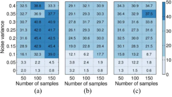
sample the same number of data points from each subspace, i.e. N1 = N2 = N3. We then add Gaussian noise with zero mean and vary the noise variance. Fig. 2 shows the average clustering error over10runs for different number of samples per subspace and different noise variance.
Fig. 2. Clustering error (%) on synthetic data when varying number of samples per subspace (x-axis) and noise variance (y-axis). (a) LRSSC. (b) GMC-LRSSC. (c)S0/`0-LRSSC.
For 50 data points per subspace and small measurement noise, S0/`0-LRSSC performs better than LRSSC and GMC-LRSSC. On the other hand, for larger measurement noise GMC-LRSSC is the best performing algorithm. When we increase the number of data poins to 100, GMC-LRSSC remains the best performing algorithm for most levels of noise. However, when further increasing number of data points,S0/`0 performs better except for very large measurement noise. This is in line with results presented in [56] which show that `0 quasi-norm regularization of least-squares problems outper-forms `p regularization 0 < p ≤ 1 for small measurement
noise. Whereas LRSSC and GMC-LRSSC in most cases do not improve performance when increasing the number of data points, S0/`0 is often able to exploit additional data.
C. Face Recognition Dataset
The Extended Yale B dataset [85], [86] consists of face images of 38 individuals (subjects). It contains 64 frontal face images of each individual acquired under different illumination conditions. We use down-sampled 48×24 pixel images and consider each vectorized image as one data point. The face images of each individual in Yale B dataset lie approximately in a 9-dimensional subspace [11].
We perform experiments for different number of clusters, ranging from 5 to 30. In each experiment we sample uniformly
L clusters from the total number of subjects and compute average of clustering error over 100 random subsets. The results are reported in Table II with the two best results high-ligted in boldface. Compared to the state-of-the-art methods, GMC-LRSSC andS0/`0-LRSSC achieve the lowest clustering error on all four clustering tasks. The difference between our algorithms and the second best performing other is significant for 10, 20 and 30 clusters (FDR<1%; Benjamini-Hochberg corrected). Importantly, by increasing the number of clusters,
TABLE II
CLUSTERING ERROR(%)ON THEEXTENDEDYALEBDATASET
L SSC LRR LRSC SSC-OMP TSC NSN LRSSC `0-SSC S2/3-LRR S1/2-LRR GMC-LRSSC S0/`0-LRSSC
5 4.54 4.38 14.56 7.46 28.38 5.42 21.19 16.27 8.94 8.92 3.97 3.52
10 8.78 7.80 34.74 15.26 39.73 9.19 26.89 28.45 9.45 9.49 4.00 4.45
20 21.52 16.68 28.23 17.23 45.57 15.02 36.78 39.24 11.98 11.58 6.38 7.14
30 26.73 21.27 31.53 20.53 47.10 18.69 33.60 39.54 12.02 11.61 8.65 8.35
the difference between our `0-based formulations and convex low-rank and sparse formulations becomes larger.
To check the effect of parameter γ in GMC-LRSSC, we vary parameter γ from 0.1 to 1, where small γ means that GMC penalty ψB is close to convex, and γ =1 corresponds
to maximally nonconvex value of the penalty. Fig. 3 shows performance as a function of γ values for 10, 20 and 30 clusters. On all these tasks, larger values of γ achieve lower clustering error than the smaller values.
Fig. 3. Clustering error on the Extended Yale B dataset for 10,20and30
clusters when varyingγparameter in GMC-LRSSC.
D. Handwritten Digit Datasets
For handwriting recognition task, we consider two datasets: MNIST and USPS datasets. Both datasets contain pictures of ten digits (0-9), each digit corresponding to one cluster. The MNIST dataset contains 10000 centered 28×28 pixel images of handwritten digits. The USPS dataset consists of 92898 handwritten digit images, each of 16×16 dimension. The handwritten digits lie approximately in a 12-dimensional subspace [87].
For both datasets, we use a subset of available images, sam-pling uniformly 50 images per digit in each run and compute average of clustering error over 100 runs. The performance comparisons for different choice of digits are shown in Table III. On both datasets,S0/`0-LRSSC and GMC-LRSSC are the only algorithms that consistently achieve high performance across varying combinations of digits.
On the MNIST dataset S0/`0-LRSSC algorithm is among the best performing algorithms, and the difference is increas-ing for larger number of clusters. GMC-LRSSC has lower performance than S0/`0-LRSSC for three combinations, but it is still significantly better than SSC, LRR and LRSSC. SSC and LRSSC have the best performance for digit sets {2,4,8}
and {2,4,6,8,9}, but they fail to give satisfactory results on other combinations of digits.
On the USPS dataset GMC-LRSSC is slightly better than
S0/`0-LRSSC, except for the combinations of five digits.
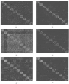
Specifically, on the digit set {2,4,6,8,9} S0/`0-LRSSC out-performs all other methods. For the hardest problems with10 clusters GMC-LRSSC and S0/`0-LRSSC again have signifi-cantly better performance (FDR<1%) than all other methods, that is 7.2% and 4.8% higher than the second best method, respectively. Fig. 4 illustrates derived affinity matrices on the USPS dataset for 10 clusters.
Fig. 4. Visualization of affinity matrices on the USPS dataset using all10
digits. (a) SSC. (b) LRR. (c) LRSSC. (d)`0-SSC. (e) GMC-LRSSC. (f)S0/`0
-LRSSC.
E. Speech Recognition Dataset
For the speech recognition task, we evaluate algorithms on the ISOLET dataset [88]. The task is to cluster subjects, where each subject spoke the name of each letter of the alphabet twice. We use dataset ISOLET1 containing 26 subjects with 30 data points from each subject. The features include spectral coefficients, contour features, sonorant, presonorant and post-sonorant features. To check whether the subspace clustering assumption holds on the ISOLET1 dataset, we compute the singular values of several subjects. Fig. 5 demonstrates that singular values decay rapidly and confirms that data points are drawn from low-dimensional subspaces.
We sample uniformly L = {5,10,15,20} clusters from the total number of subjects over 100 random subsets. The average clustering errors are reported in Table IV. For all tested numbers of clustersS0/`0-LRSSC is the best performing
TABLE III
CLUSTERING ERROR(%)ONMNISTANDUSPSDATASETS
Digits Dataset SSC LRR LRSC SSC- TSC NSN LRSSC `0-SSC S2/3- S1/2- GMC- S0/`0 -OMP LRR LRR LRSSC LRSSC 2,4,8 MNIST 7.43 14.14 10.59 11.06 12.09 13.02 7.01 7.82 14.80 15.03 8.66 8.92 USPS 6.02 10.37 7.61 21.04 8.32 18.67 7.13 4.88 8.83 9.70 4.92 6.40 3,6,9 MNIST 3.89 3.49 4.61 5.69 3.25 2.99 4.15 3.49 5.93 6.61 2.93 3.25 USPS 2.05 1.57 4.50 23.43 1.43 2.22 8.13 1.09 3.02 3.68 0.97 1.27 1,4,7 MNIST 47.50 45.09 44.14 42.21 33.72 14.05 47.09 45.40 43.42 42.57 34.50 27.33 USPS 2.21 4.01 4.33 58.07 7.45 9.45 8.61 3.68 4.27 5.37 2.65 3.82 2,4,6,8,9 MNIST 25.54 33.54 29.22 29.43 28.95 27.04 26.78 28.94 34.90 36.29 27.40 27.20 USPS 15.69 22.30 18.86 53.43 20.35 26.69 18.67 14.31 19.22 19.95 15.37 13.38 0,1,3,5,7 MNIST 53.60 33.61 35.92 37.51 30.16 22.39 46.86 33.74 32.50 33.08 29.80 27.85 USPS 30.00 22.83 28.47 74.66 25.58 13.36 35.44 30.17 27.41 27.68 24.76 10.89 0-9 MNIST 47.49 45.13 46.88 46.45 40.00 34.81 45.68 39.51 43.19 43.66 38.01 34.89 USPS 28.28 33.44 28.58 84.01 29.34 28.43 33.10 27.27 28.75 29.24 20.46 22.45 TABLE IV
CLUSTERING ERROR(%)ON THEISOLET1DATASET
L SSC LRR LRSC SSC-OMP TSC NSN LRSSC `0-SSC S2/3-LRR S1/2-LRR GMC-LRSSC S0/`0-LRSSC
5 10.98 7.61 10.25 27.79 11.58 8.23 8.63 9.23 7.45 8.06 7.07 6.87
10 17.11 14.65 15.84 44.44 19.35 16.04 14.72 18.21 14.10 14.34 13.92 13.81
15 25.64 23.14 22.88 54.03 27.07 23.61 23.87 25.73 20.37 20.24 20.29 19.90
20 31.05 30.60 27.93 59.89 31.70 27.94 29.90 30.28 26.02 25.24 25.32 25.07
Fig. 5. Singular values of several speakers on the ISOLET1 dataset.
method. GMC-LRSSC is the second best method for 5 and 10clusters, while for15and20it achieves the same result as Schatten-2/3 and Schatten-1/2LRR.
F. Computational Time and Convergence
We further test the convergence behavior of GMC-LRSSC and S0/`0-LRSSC. The convergence conditions of GMC-LRSSC are satisfied within less than 15 iterations on all four real-world datasets. Fig. 6 illustrates convergence behavior of GMC-LRSSC on the MNIST and ISOLET1 datasets for 10 clusters. S0/`0-LRSSC converges within 20 iterations on the Extended Yale B, MNIST and USPS datasets. Fig. 7 shows behavior ofS0/`0-LRSSC on the MNIST and ISOLET1 datasets for 10 clusters. Although the maximal number of iterations is exceeded on the ISOLET1 dataset, Fig. 7 shows that the error decays rapidly and within 20 iterations.
The average computational time over 100 runs of each algorithm is shown in Table V. On all datasets, LRSC is consistently the fastest algorithm. GMC-LRSSC is among the fastest algorithms, whereasS0/`0-LRSSC is among the fastest
algorithms on the Extended Yale B and MNIST datasets. As explained above, on ISOLET1 dataset S0/`0-LRSSC exceeds maximum number, resulting in higher computational time. All experiments were run in MATLAB 2017a environment on the PC with256 GB of RAM and Intel Xeon CPU E5-2650 v42 processors operating with a clock speed of2.2 GHz.
Fig. 6. Convergence of GMC-LRSSC. (a) MNIST dataset. (b) ISOLET1 dataset.
Fig. 7. Convergence of S0/`0-LRSSC. (a) MNIST dataset. (b) ISOLET1
TABLE V
AVERAGE TIME(S)ON THEEXTENDEDYALEB, MNISTANDISOLET1DATASETS
Dataset L SSC LRR LRSC SSC- TSC NSN LRSSC `0-SSC S2/3- S1/2- GMC- S0/`0 -OMP LRR LRR LRSSC LRSSC Yale B 5 30.88 10.21 0.18 0.56 0.44 1.28 10.65 40.11 9.85 10.02 0.39 0.59 10 54.30 31.52 0.41 1.29 1.00 2.94 69.97 101.00 33.78 34.32 1.86 2.91 30 180.67 271.52 2.47 6.29 6.20 14.84 642.33 623.94 295.74 297.36 19.19 29.24 MNIST 3 0.56 1.17 0.05 0.15 0.17 0.52 0.37 2.63 1.35 1.37 0.12 0.11 5 1.31 4.01 0.10 0.27 0.29 0.85 1.40 5.11 5.03 5.10 0.30 0.26 10 4.59 13.56 0.26 0.60 0.67 1.83 12.44 14.37 17.09 17.41 1.45 1.18 ISOLET1 5 6.83 4.78 0.09 0.20 0.25 0.60 4.24 4.71 5.99 6.12 0.41 2.36 10 14.23 17.23 0.26 0.47 0.61 1.31 30.05 12.82 21.78 22.21 1.87 12.95 20 38.37 30.34 0.28 1.17 1.64 3.05 133.86 45.79 34.05 34.87 6.96 50.93
VI. CONCLUSION ANDDISCUSSION
In this paper we have introduced two nonconvex regulariza-tions in low-rank sparse subspace clustering: (i) multivariate generalization of minimax-concave penalty function; and (ii)
S0/`0 regularization with a proximal operator approximated using the proximal average method. Under the proposed framework, we have presented two algorithms based on the alternating direction method of multipliers. We have per-formed extensive experiments on synthetic and four real world datasets, including face recognition, handwriting recognition and speech recognition tasks. Our experimental results have shown that both proposed methods converge fast and achieve clustering error lower than nuclear and `1 norms regularized objective. Moreover, for larger number of clusters proposed methods consistently outperform existing subspace clustering methods. That is explained by their more accurate approxi-mation of rank and sparsity of the data representation matrix than it is the case with nuclear and`1 norms.
The choice of norm should be decided depending on the dataset. In future work we plan to study how different ini-tializations affect the accuracy of the proposed nonconvex regularization based methods. Instead of directly solving NP hard`0quasi-norm minimization problem, we are interested in finding a way to gradually build a solution. A possible strategy could be to start with`1norm solution. Since analytic formulas for thresholding function exist for p=1/2 and p=2/3[89], we can gradually shrink p and use the current solution to initialize the next step of the algorithm. This approach is called
p-continuation strategy in [56].
APPENDIX
PROOF OFPROPOSITION2ANDTHEOREM1 In this section, we first prove the boundedness of variables in Algorithm 1. This result helps us to establish convergence property of Algorithm 1. We then prove Theorem 1 in the paper, where we show that any converging point satisfies Karush-Kuhn-Tucker (KKT) conditions [78].
Proof of Proposition 2:
From the first order optimality conditions of Lagrangian
function in (25) we have: 0∈∂C1Lµ1k,µ2k J k+1,Ck+1 1 ,C k+1 2 ,Λ k 1,Λ k 2 0∈∂C2Lµk 1,µ k 2 J k+1,Ck+1 1 ,C2k+1,Λk1,Λk2 . (49)
The optimality condition of problem in (30) implies that:
∂τψ
B Ck2+1 i j−Λ2k+1i j =0, (50) where ∂ψB C2k+1 i j denotes gradient of the GMC penalty
ψB at C2k+1i j. By the definition of the scaled MC penalty in (22) and using B=qµk 2γ/τI we have: ∂φb ci j= sign(ci j) − µk 2γ τ ci j, if |ci j| ≤ µτk 2γ 0, if |ci j| >µτk 2γ , (51) whereci j denotes C2 i j.
If |ci j| > τ/(µk2γ), then from (50) and (51) directly follows
Λk2+1i j =0.
Otherwise, we get the following equality:
Λk2+1 i j=sign C2k+1i j − µ k 2γ τ C2k+1i j. (52) Since Ck+1 2 i j ≤ τ/(µk2γ), it follows Λk2+1 i j ≤ 1.
Therefore, sequence Λk2 is bounded.
The optimality condition of problem in (28) implies that:
∂λψ B σ C1k+1 i j− Λk1+1 i j=0, (53)
Similarly, following the proof for C2 and using Proposition 1, it can be shown that the sequence
Λk1 is also bounded. Using the definitions of Jk+1,Ck+1
1 andC
k+1
2 as minimizers, we have the following inequalities [90]:
Lµk 1,µ k 2 J k+1,Ck+1 1 ,C k+1 2 ,Λ k 1,Λ k 2 ≤ Lµk 1,µ k 2 J k+1,Ck+1 1 ,C2k,Λk1,Λk2 ≤ Lµk 1,µ k 2 J k+1,Ck 1,C k 2,Λ k 1,Λ k 2 ≤ Lµk 1,µ k 2 J k,Ck 1,C k 2,Λ k 1,Λ k 2 . (54)
Note that the last term equals: Lµk 1,µ k 2 J k,Ck 1,C k 2,Λ k 1,Λ k 2 =Lµk−1 1 ,µ k−1 2 J k,Ck 1,C k 2,Λ k−1 1 ,Λ k−1 2 + 2 Õ i=1 aikΛki −Λ k−1 i k 2 F, (55) where ai = µk i+µ k−1 i 2(µk−1 i ) 2, i = 1,2. Since µk = ρµk −1, ρ > 1, it follows that µk is non-decreasing andÍ∞
k=0µ1k i <∞,i=1,2. We then have: ∞ Õ k=1 µk i +µk −1 i 2(µk−1 i ) 2 = ∞ Õ k=1 1+ρ 2µk−1 i <∞. (56) Since Λk1 and
Λk2 are bounded, then
kΛk1 −Λk1−1k2
F
and
kΛk1 − Λ1k−1kF2 in (55) are also bounded. Therefore, from (54), (55) and (56) follows that
Lµk 1,µ k 2 J k+1,Ck+1 1 ,C k+1 2 ,Λ k 1,Λk2 is upper-bounded. Furthermore, it holds that:
1 2 X−X Jk 2 F+λψB(σ(C k 1))+τψB(C2k) =Lµk−1 1 ,µ k−1 2 J k,Ck 1,C2k,Λk −1 1 ,Λk −1 2 −1 2 Λk1 2 F− Λ1k−1 2 F µk−1 1 −1 2 Λk2 2 F− Λk2−1 2 F µk−1 2 (57) Since Lµk−1 1 ,µ k−1 2 J k,Ck 1,C k 2,Λ k−1 1 ,Λ k−1 2 is upper-bounded andΛk1 andΛk2 are both bounded, Jk is also bounded.
The boundedness of
Ck
1 and
Ck
2 follows from the update rules for Lagrange multipliers in(33)and boundedness of Jk , Λk1 , and Λk2 . Therefore, sequence Jk,C1k,C2k,Λ1k,Λk2 generated by Algorithm 1 is bounded. Bolzano-Weierstrass theorem [91] then guarantees the existence of a convergent subsequence.
Proof of Theorem 1: Let J∗,C∗1,C2∗,Λ∗1,Λ∗2
be a critical point of (24). The KKT conditions are derived as follows:
(1) J∗−C∗1=0, (2) J∗−C∗2=0, (3) −XT X−X J∗+ Λ∗1+Λ∗2=0 (4) Λ∗1 ∈∂C 1λψB σ(C ∗ 1) (5) Λ∗2 ∈∂C 2τψB C ∗ 2 . (58)
From the 1st and 4th KKT conditions, it follows: J∗+Λ ∗ 1 µ∗ 1 ∈J∗+ µλ∗ 1 ∂C 1ψB σ(C ∗ 1) =C∗1+ λ µ∗ 1 ∂C 1ψB σ(C ∗ 1) . (59)
Let U1Σ1V1T be the SVD of matrix C1∗. Using Proposition 1,
the right hand side of (59) equals: C1∗+ λ µ∗ 1 ∂C1ψB σ(C ∗ 1) = U1Σ1V1T+ λ µ∗ 1 U1∂Σ1 ψB Σ1 V T 1 =U1 Σ1+ λ µ∗ 1 ∂Σ1 ψB Σ1 V T 1 ,U1Qa1,b1 Σ1 V1T, (60) where a1 = µ∗1/λ and b1 = q µ∗ 1γ/λ, 0 < γ ≤1. The scalar functionQa,b is defined asQa,b(x),x+1a∂φb(x), where φb
is the scaled MC penalty defined in (22).Qa1,b1(x)is applied element-wise to singular values of matrixC∗
1. Let U2Σ2V2T be the SVD of matrix J∗ +Λ∗1/µ
∗ 1
. From (59), we get the following relation:
U2Σ2V2T ∈U1Qa1,b1 Σ1
V1T. (61) It is easy to verify that Qa1,b1 is a monotone function [92], [93] andQ−1a 1,b1(x)=Θ x; λ µ∗ 1 , λ γµ∗ 1 for 0< γ≤1, whereΘis the firm thresholding function defined in (1). ApplyingQ−1a
1,b1 to both sides of (61) and replacingU1Σ1V1T =C∗1, we get:
C∗1=U2Q−a11,b1 Σ2 V2T =U2Θ Σ2;µλ∗ 1 , λ γµ∗ 1 V2T. (62) Similarly, from the 2nd and 5th KKT conditions, we have the following relations: J∗+Λ ∗ 2 µ∗ 2 ∈J∗+ τ µ∗ 2 ∂C2ψB C ∗ 2 =C∗2+ τ µ∗ 2 ∂C2ψB C ∗ 2 ,Qa2,b2 C ∗ 2), (63) wherea2 =µ∗2/τ andb2 = q µ∗ 2γ/τ,0< γ≤1. Again, applying Q−1a
2,b2 to both sides of (63), we get the following equations: C∗2=Q−1a 2,b2 J∗+Λ ∗ 2 µ∗ 2 =ΘJ∗+Λ ∗ 2 µ∗ 2 ; µτ∗ 2 , τ γµ∗ 2 . (64) Therefore, the 4th and 5th KKT conditions can be rewritten as: (4) C1∗=U2Θ Σ2;µλ∗ 1 , λ γµ∗ 1 V2T (5) C2∗=Θ J∗+Λ ∗ 2 µ∗ 2 ; τ µ∗ 2 , τ γµ∗ 2 . (65)
We now show that KKT conditions are satisfied when assumptions of Theorem 1 hold. From (33) we have:
Λk1+1−Λk1 =µ1k Jk+1−C1k+1
Λk2+1−Λk2 =µk2 Jk+1−C2k+1. (66)
Since by the assumption Λk1+1−Λk1
→0and Λk2+1−Λk2
→ 0, then the first two KKT conditions are satisfied.
From the update rule in (27), we have:
XTX+(µk1+µk2)I Jk+1−Jk =µk 1 C1k−Jk +µk 2 C2 k−Jk −Λ1k−Λ2k+XT X−X Jk. (67)
From the the first two conditions, it follows that when Jk+1− Jk →0, the 3rd KKT condition is satisfied.
Next, using the update for C1 in (29) we obtain the following equation: C1k+1−C1k =U2Θ Σ2; λ µk 1 , λ γµk 1 V2T−Ck1, (68) whereU2Σ2V2T is the SVD of matrix Jk+1+Λ1k/µk1. From the update rule for C2 in (32) it follows:
C2k+1−C2k =Θ Jk+1+Λ k 2 µk 2 ; τ µk 2 , τ γµk 2 −C2k. (69) WhenC1k+1−C1k →0andC2k+1−Ck2 →0, follow the equations in (65). Since Yk ∞
k=1 is bounded and equations (66), (67), (68), (69) go to zero, we conclude that the sequence Yk ∞k=1
asymptotically satisfies the KKT conditions in (58).
ACKNOWLEDGMENT
The authors would like to thank Shin Matsushima for his helpful comments on improving the statements of Proposition 2 and Theorem 1. The authors would also like to thank the Editor and reviewers for their comments which helped to improve this paper.
REFERENCES
[1] X. Wang and X. Tang, “A unified framework for subspace face recog-nition,” IEEE Trans. Pattern Anal. Mach. Intell., vol. 26, no. 9, pp. 1222–1228, 2004.
[2] J. Wright, A. Y. Yang, A. Ganesh, S. S. Sastry, and Y. Ma, “Robust face recognition via sparse representation,”IEEE Trans. Pattern Anal. Mach. Intell., vol. 31, no. 2, pp. 210–227, 2009.
[3] S. Rao, R. Tron, R. Vidal, and Y. Ma, “Motion segmentation in the presence of outlying, incomplete, or corrupted trajectories,”IEEE Trans. Pattern Anal. Mach. Intell., vol. 32, no. 10, pp. 1832–1845, 2010. [4] F. de Morsier, M. Borgeaud, V. Gass, J. P. Thiran, and D. Tuia,
“Kernel low-rank and sparse graph for unsupervised and semi-supervised classification of hyperspectral images,” IEEE Trans. Geosci. Remote Sens., vol. 54, no. 6, pp. 3410–3420, 2016.
[5] H. Song, W. Yang, N. Zhong, and X. Xu, “Unsupervised classification of polsar imagery via kernel sparse subspace clustering,”IEEE Geosci. Remote Sens. Lett., vol. 13, no. 10, pp. 1487–1491, 2016.
[6] A. W.-C. Liew, N.-F. Law, and H. Yan, “Missing value imputation for gene expression data: computational techniques to recover missing data from available information,”Brief. Bioinf., vol. 12, no. 5, pp. 498–513, 2011.
[7] R. Vidal, “Subspace clustering,” IEEE Signal Process. Mag., vol. 28, no. 2, pp. 52–68, 2011.
[8] J. Shi and J. Malik, “Normalized cuts and image segmentation,”IEEE Trans. Pattern Anal. Mach. Intell., vol. 22, no. 8, pp. 888–905, 2000. [9] A. Y. Ng, M. I. Jordan, and Y. Weiss, “On spectral clustering: Analysis
and an algorithm,” inAdvan. Neural Inf. Process. Syst. 14, 2001, pp. 849–856.
[10] U. von Luxburg, “A tutorial on spectral clustering,” Stat. Comput., vol. 17, no. 4, pp. 395–416, 2007.
[11] E. Elhamifar and R. Vidal, “Sparse subspace clustering: Algorithm, theory, and applications,” IEEE Trans. Pattern Anal. Mach. Intell., vol. 35, no. 11, pp. 2765–2781, 2013.
[12] X. Peng, Z. Yu, Z. Yi, and H. Tang, “Constructing the L2-graph for robust subspace learning and subspace clustering,”IEEE Trans. Cybern., vol. 47, no. 4, pp. 1053–1066, 2017.
[13] G. Liu and Y. Lin, Z. annd Yu, “Robust subspace segmentation by low-rank representation,” in26th Int. Conf. Mach. Learn., 2010, pp. 663–670. [14] G. Liu, Z. Lin, S. Yan, J. Sun, Y. Yu, and Y. Ma, “Robust recovery of subspace structures by low-rank representation,”IEEE Trans. Pattern Anal. Mach. Intell., vol. 35, no. 1, pp. 171–184, 2013.
[15] J. Wang, X. Wang, F. Tian, C. H. Liu, and H. Yu, “Constrained low-rank representation for robust subspace clustering,” IEEE Trans. Cybern., vol. 47, no. 12, pp. 4534–4546, 2017.
[16] C. G. Li and R. Vidal, “A structured sparse plus structured low-rank framework for subspace clustering and completion,”IEEE Trans. Signal Process., vol. 64, no. 24, pp. 6557–6570, 2016.
[17] P. Favaro, R. Vidal, and A. Ravichandran, “A closed form solution to robust subspace estimation and clustering,” inIEEE Conf. Comput. Vision Pattern Recognit., 2011, pp. 1801–1807.
[18] E. J. Candès and B. Recht, “Exact matrix completion via convex optimization,”Found. Comput. Math., vol. 9, no. 6, p. 717, 2009. [19] E. J. Candès and T. Tao, “The power of convex relaxation: Near-optimal
matrix completion,”IEEE Trans. Inf. Th., vol. 56, no. 5, pp. 2053–2080, 2010.
[20] E. J. Candès, X. Li, Y. Ma, and J. Wright, “Robust principal component analysis?”J. ACM (JACM), vol. 58, no. 3, p. 11, 2011.
[21] E. Elhamifar and R. Vidal, “Sparse subspace clustering,” inIEEE Conf. Comput. Vision Pattern Recognit., 2009, pp. 2790–2797.
[22] E. J. Candès and T. Tao, “Decoding by linear programming,” IEEE Trans. Inf. Th., vol. 51, no. 12, pp. 4203–4215, 2005.
[23] D. L. Donoho, “For most large underdetermined systems of linear equations the minimal `1-norm solution is also the sparsest solution,”
Commun. Pure Applied Math., vol. 59, no. 6, pp. 797–829, 2006. [24] K. Tang, R. Liu, Z. Su, and J. Zhang, “Structure-constrained low-rank
representation,”IEEE Trans. Neural Netw. Learn. Syst., vol. 25, no. 12, pp. 2167–2179, 2014.
[25] K. Tang, D. B. Dunsonc, Z. Sub, R. Liub, J. Zhanga, and J. Dong, “Subspace segmentation by dense block and sparse representation,” Neural Netw., vol. 75, no. 1, pp. 66–76, 2016.
[26] E. Elhamifar and R. Vidal, “Clustering disjoint subspaces via sparse representation,” inIEEE Int. Conf. Acoustics, Speech Signal Process., 2010, pp. 1926–1929.
[27] B. Nasihatkon and R. Hartley, “Graph connectivity in sparse subspace clustering,” inIEEE Conf. Comput. Vision Pattern Recognit., 2011, pp. 2137–2144.
[28] L. Zhuang, H. Gao, Z. Lin, Y. Ma, X. Zhang, and N. Yu, “Non-negative low rank and sparse graph for semi-supervised learning,” inIEEE Conf. Comput. Vision Pattern Recognit., 2012, pp. 2328–2335.
[29] Y.-X. Wang, H. Xu, and C. Leng, “Provable subspace clustering: When LRR meets SSC,” in Advan. Neural Inf. Process. Syst. 26, 2013, pp. 64–72.
[30] M. Brbi´c and I. Kopriva, “Multi-view low-rank sparse subspace cluster-ing,”Pattern Recognit., vol. 73, pp. 247–258, 2018.
[31] D. L. Donoho and M. Elad, “Optimally sparse representation in general (nonorthogonal) dictionaries via`1minimization,”Proc. Natl. Acad. Sci,
vol. 100, no. 5, pp. 2197–2202, 2003.
[32] V. Larsson and C. Olsson, “Convex low rank approximation,” Int. J. Comput. Vision, vol. 120, no. 2, pp. 194–214, 2016.
[33] A. Parekh and I. W. Selesnick, “Enhanced low-rank matrix approxima-tion,”IEEE Signal Process. Lett., vol. 23, no. 4, pp. 493–497, 2016. [34] I. Selesnick, “Sparse regularization via convex analysis,”IEEE Trans.
Signal Process., vol. 65, no. 17, pp. 4481–4494, 2017.
[35] C. Lu, J. Tang, S. Yan, and Z. Lin, “Generalized nonconvex nonsmooth low-rank minimization,” inIEEE Conf. Comput. Vision Pattern Recog-nit., 2014, pp. 4130–4137.
[36] C. Lu, C. Zhu, C. Xu, S. Yan, and Z. Lin, “Generalized singular value thresholding,” inProc. the 29th AAAI Conf. Artif. Intell., ser. AAAI’15. AAAI Press, 2015, pp. 1805–1811.
[37] M. Malek-Mohammadi, M. Babaie-Zadeh, and M. Skoglund, “Iterative concave rank approximation for recovering low-rank matrices,” IEEE Trans. Signal Process., vol. 62, no. 20, pp. 5213–5226, 2014. [38] M. Kliesch, R. Kueng, J. Eisert, and D. Gross, “Improving compressed
sensing with the diamond norm,”IEEE Trans. Inf. Th., vol. 62, no. 12, pp. 7445–7463, 2016.
[39] C. Lu, J. Tang, S. Yan, and Z. Lin, “Nonconvex nonsmooth low rank minimization via iteratively reweighted nuclear norm,” IEEE Trans. Image Process., vol. 25, no. 2, pp. 829–839, 2016.
[40] X. T. Yuan and Q. Liu, “Newton-type greedy selection methods for
`0-constrained minimization,”IEEE Trans. Pattern Anal. Mach. Intell.,
vol. 39, no. 12, pp. 2437–2450, 2017.
[41] R. Peharz and F. Pernkopf, “Sparse nonnegative matrix factorization with`0-constraints,”Neurocomput., vol. 80, pp. 38–46, 2012.
[42] T. Blumensath and M. E. Davies, “Iterative hard thresholding for compressed sensing,”Applied Comput. Harm. Anal., vol. 27, no. 3, pp. 265–274, 2009.