Information encoding by deep neural networks: what can we learn?

Information encoding by deep neural networks: what can we learn?

L. ten Bosch

_{, L. Boves}

1

_{Radboud University Nijmegen, NL;}

_{Max Planck Institute for Psycholinguistics}

Abstract

The recent advent of deep learning techniques in speech tech-nology and in particular in automatic speech recognition has yielded substantial performance improvements. This suggests that deep neural networks (DNNs) are able to capture structure in speech data that older methods for acoustic modeling, such as Gaussian Mixture Models and shallow neural networks fail to uncover. In image recognition it is possible to link repre-sentations on the first couple of layers in DNNs to structural properties of images, and to representations on early layers in the visual cortex. This raises the question whether it is possi-ble to accomplish a similar feat with representations on DNN layers when processing speech input. In this paper we present three different experiments in which we attempt to untangle how DNNs encode speech signals, and to relate these repre-sentations to phonetic knowledge, with the aim to advance con-ventional phonetic concepts and to choose the topology of a DNNs more efficiently. Two experiments investigate represen-tations formed by auto-encoders. A third experiment investi-gates representations on convolutional layers that treat speech spectrograms as if they were images. The results lay the basis for future experiments with recursive networks.

Index Terms: deep neural networks, conventional knowledge, information encoding, structure discovery

1. Introduction

The speech technology field is being revolutionized by the ap-plication of deep learning techniques, in particular Deep Neural Nets (DNNs). DNNs, in various forms, are now being applied for many tasks in automatic speech processing. Their success in terms of conventional performance measures suggests that the parameters of a trained DNN reflect relevant structure in the training data.

The question how information is ‘covered’ or ‘represented’ in a trained DNN is long-standing [1, 2, 3, 4, 5, 6], but it is still not trivial to see whether and how a trained DNN can be interpreted and howwemight be able to learn from DNNs. The ability to interpret trained DNNs might advance, and perhaps revolutionize, our understanding of the phonetic or linguistic structure of speech.

In recent studies, the question how information can be en-coded in DNNs is addressed in different ways.

First, DNNs may discover structure in data sets because subsequent layers ignore more and more details that are irrele-vant for correctly predicting output labels [7, 8]. Increasingly abstract representations emerge by cascading multiple (non-linear) transformations [9]. Recent DNN classification results show that this interpretation is most convincing in image clas-sification tasks. The idea of each layer representing a more ab-stract representation of the input can be interpreted in terms of a mappingffrom the input spaceX to an output spaceY. If

this mapping can be decomposed as a cascade of sub-mappings,

e.g.,Y =g(f(X))(in whichf()represents the mapping from

Xto an unobservable (hidden, latent) spaceH, andg()a map-ping fromHtoY), this decomposition may directly be reflected

by a multilayer topology, and vice versa.

Alternatively, papers such as [10] focus on the role of DNNs to find optimal representations, in particular in the sense of fea-tures. They argue that learning of optimal representations can be achieved if the network is able to disentangle the underlying explanatory factors hidden in the observed data. This approach may be especially interesting when the data emerge from the in-teraction between many sources. However, as admitted in [10], it is as yet unclear how meta-level knowledge about underly-ing sources of variation can be brought to bear in designunderly-ing optimal training methods, and in interpreting trained networks. The layer-idea and the representation approach come back in the first experiment in this paper (see below).

A third, more geometrically inspired interpretation of the input-output relation in a DNN is based on the manifold as-sumption, which holds that data in the input space are all mapped to the vicinity of a manifold M of typically a much lower (functional) dimensionality embedded in a high dimen-sional embedding space (e.g. [1, 11, 10]). The application of manifold learning methods on speech signals [2] is motivated by the argument that speech is produced by relatively slow bal-listic movements of articulators. By modeling manifolds by a monotonic chain of simpler spatial forms, [12] showed that DNNs can represent data that lie on a low-dimensional mani-fold with great accuracy, suggesting that deep networks provide a very effective method for dimensionality reduction. To a first approximation, directions tangent to the manifold are well pre-served while directions orthogonal to the manifolds aren’t. This idea comes back in the second and third experiment in this paper.

A fourth approach is more theoretical and analyzes DNNs on an ‘information plane’, by invoking the notion of the ‘in-formation bottleneck’ [13]. Any DNN can be characterized by the mutual information between a hidden layer and the input and output variables, as a function of hidden layer depth. The resulting mutual information values are related via a chain of inequalities [13]. Tishby and colleagues [8] argue that the opti-mal architecture (number of layers and features/connections at each layer) is related to the bifurcation points of the informa-tion bottleneck trade-off (i.e., the amount of compression from the input layer to a hidden layer as a function of hidden layer depth). The hierarchical representations then correspond to the phase transitions related to these bifurcation points. In this vein, even more abstract approaches are being investigated, e.g. [14].

1.1. Description of our experiments

We describe three interrelated experiments that aim at unrav-eling the information captured in a trained DNN in different ways. Following the reasoning in [15] and the approach in [13], all DNNs are chosen to be relatively small: if it appears

diffi-Interspeech 2018

cult or impossible to unravel information from a DNN with a limited number of layers, it will be an uphill battle to extract information from larger networks. Our aim here, therefore, is mainly to provide a proof of principle.

The first experiment employs a Convolutional Neural Net (CNN) (cf. [16]) implemented in TensorFlow [17] and re-uses the data and method described in the low-footprint keyword spotting task [18]. It investigates the convolution matrices that are constructed in the first hidden layer of the resulting CNN, while varying the number of hidden units in the first and second hidden layer.

The second experiment investigates the representation on a bottleneck layer in a stacked autoencoder used on TIMIT, and focuses on the distribution of the bottleneck representations aligned with the TIMIT phone segmentation. The evolution of the statistical distribution of the phone classes using bottleneck representations is studied during learning.

The third experiment also applies stacked autoencoders on TIMIT. Following ideas in [9, 13, 8], we investigate the com-monstructure in bottleneck representations obtained in indepen-dently trained auto-encoders with the same topology. As might be expected, while the I/O relations of these networks are very similar (with very high correlations between the resulting out-puts for the same input), the internal bottleneck representations are very different.

2. Terminology, notation

The DNNs that we consider are either CNNs or stacked autoen-coders. The input and output space are denotedX andY,

re-spectively. Hidden layers at depthispan the space denotedHi

(or justH, when there is no confusion). If a bottleneck layer

H of an autoencoder has a dimensiondim(H)<dim(X) = dim(Y), the encoder mappingE can be considered as a sub-jective function fromXontoH; the decoder mappingDis an injective function fromH to Y (D : _H ,_{→ Y}). The image

D(_H) _{⊂ Y}is a manifold embedded inY with functional di-mension at mostdim(H).

3. Experiments

3.1. Convolutional matrices: the ears and noses

We re-used the DNN and the training data from [18]; the DNN was implemented using Tensorflow [17]. Leaving aside all de-tails here, the network consists of two convolutional layers, fol-lowed by a fully connected layer which seeds into a softmax output layer. The network is adapted from a visual classifica-tion system, which explains why the input consists of fixed-sized spectrograms (all training and test utterances must have a duration of exactly 1 s). TensorFlow provides relatively easy ac-cess to the trained convolution filters and to the representations formed at the convolution layers given a test utterance. The di-mensions of the convolution filters and the number of nodes in the layers are parameters. We kept the dimensions of the filters fixed, but varied the number of nodes in the layers, to investi-gate whether increasing this number would expose increasingly more detailed (and interpretable) spectro-temporal structures. After CNN training, we selected thenh(2, 4, 8, 16, 32)

con-volution matrices of size20by8(time·freq), each associated to each of thenhnodes in the first hidden layer. Each value ofnh

thus generates a ‘generation’ of convolution matrices.

It might be expected that convolution matrices are not ran-domly positioned, but instead that matrices in the ‘next’

gener-Figure 1: The genealogy of convolution matrices on the first hidden layer. The CNN used is from [18]. At the left, the two convolution matrices are presented that result form a training with 2 hidden nodes on the first hidden layer. The next column contains the four convolution matrices resulting from a training with four hidden nodes, etc.

ation (fornh) in some way ‘improve’ the matrices in the

pre-vious generation (fornh/2). Due to the dotprod operation in

the CNN, these matrices can be interpreted as weightings in the spectro-temporal domain. By using the angle between the ma-trices as between-matrix distance (i.e., a distance closely related to the dotprod operation) it appears that the matrices obtained for lownh(2, 4, 8, 16 and 32) can be arranged in a balanced

hi-erarchical structure: after linking each matrix in the next ‘gener-ation’ to its closest parent matrix from the previous generation, often each parent appears to link with exactly 2 matrices in the next generation.

The corresponding specialization tree fornh= 2,4,8,16

is depicted in fig. 1. At the left, the two convolution matrices are shown in the casenh= 2. The next column contains the four

convolution matrices resulting from a training withnh = 4;

also the links to the closest ‘parent’ are depicted. Ramification takes place from left to right (details omitted for the sake of clar-ity). The resulting convolution matrices clearly show a time-frequency structure, somewhat similar to the ‘ears and noses’ observed in the first hidden layer of the well-known face classi-fication networks. The interaction between time and frequency (similar to the Gabor patterns) can be interpreted as primitive shape descriptions of spectral (formant) transitions, with simi-larities to the results [6] that were obtained by combining speech and image input data.

3.2. Dynamics in bottleneck representations

In the second experiment we focus on the phonetic represen-tation on the bottleneck layer in a DNN trained on TIMIT. Here we study how well vowels, semivowels, liquids, frica-tives, nasals and plosives can be separated by computing the Kullback-Leibler (KL) dissimilarity in the bottleneck represen-tations related to each phone-pair, as a function of epoch. The phone-phone KL measure was computed using gaussmixk.m (VoiceBox, [19]), in which each class is first estimated using a Gaussian mixture and next the KL dissimilarity between both classes is estimated. Albeit an approximation, it provides an adequate alternative for the (less tractable) analytical approach. For the sake of feasibility, the DNN consisted of two stacked autoencoders with hidden layers of size 8 and 5, respec-tively. The resulting DNN has three hidden layers, with dimen-sion 8, 5 (bottleneck), and 8, respectively. Each autoencoder training was characterized by a L2 Weight Regularization equal

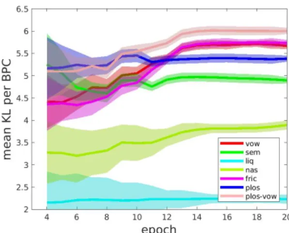
Figure 2: This figure shows, for 7 broad phonetic classes (BPCs), the improvement of the average KL dissimilarity within a BPC, as function of training epoch. The KL dissimilarity is computed on the basis of the DNN’s bottleneck representation. For the sake of comparison, the top plot shows the KL dissim-ilarity between very distinct BPCs (vowels and plosives), as function of epoch. The bands around these plots show the vari-ation around the averages, as observed across 16 independent DNN optimization runs.

to 0.01, a Sparsity Regularization equal to 4, and a sparsity pro-portion of 0.05. All encoder transfer functions were ‘logsig’ (f(x) = 1/(1 + exp(₋x)), and the decoder transfer function was ‘purelin’ (f(x) =x).

The input spaceX was chosen to be sequence of single-MFCC vectors of dimension 13 (c0, . . . , c12), after mean sub-traction per utterance. For each component, the variance was kept. Since the DNNs used here are less deep than the Deep belief networks used in other studies (e.g., [20]) we chose the (already orthogonalized) MFCC representations rather than the log energies per Mel-band.

Instead of displaying raw confusion matrices, we focus on the average phone-phone KL dissimilarity within each of the 6 broad phonetic classes (BPC): vowels, semivowels, liquids, fricatives, nasals and plosives. These averages, measured on the basis of the bottleneck representation, are shown in Fig. 2 as a function of epoch (here, ‘epoch’ is a unit of 20 consecu-tive DNN training iterations). For the sake of comparison, the top plot shows the KL dissimilarity between very distinct BPCs (vowels and plosives); this is near ceiling.

In order to study robustness, we performed the same train-ing a number of times. The transparent bands show the varia-tion around the averages, as obtained from 16 independent DNN training runs with different optimization settings. The pattern-ing suggests that the acoustic-phonetic information in the bot-tleneck unfolds in the same way for DNNs sharing the same topology.

The figure shows that the phones within each BPC get better separable during training. Vowels and fricatives are best separa-ble within their BPC, followed by plosives, semivowels, nasals and finally liquids. However, rates of improvement differ by a factor of around 3 to 4 during certain periods of the training. It appears that the best performing BPCs primarily profit from a steep rise during the first part of the training, while lower-performing BPCs such as nasals and liquids lack this speed rise and show a very shallow increase in performance across the

Figure 3:Example of predictions in the output spaceY.

Origi-nalc1(dashed, red) and a number ofc1-predictions (solid) from independently trained different DNNs.

entire training. In general, low performing BPCs also show a much larger variation across different training runs compared to better performing BPCs. This difference between BPCs cannot be attributed to frequency of occurrence of the phone tokens; instead, it is likely that this difference has to do with how ‘en-tangled’ the phone encoding is in the bottleneck space. This will be addressed in the third experiment.

3.3. Are bottleneck representations diffeomorphic?

In the third experiment we focus on the bottleneck layerHwith dimensionnh, but from another viewpoint: we compare

differ-ent bottleneck represdiffer-entations in separately trained DNNs that share the same topology (8−nh−8). Similar to the previous

experiment, the DNNs were set-up as autoencoders on TIMIT and used the ‘tansig’ function as transfer function and the ‘pure-lin’ from the last hidden layer to the output layer. There was no regularization: no additional constraints were imposed on the hidden representations.

The DNNs have the freedom to implement the mapping from input space (X)to output space (Y) in multiple ways (e.g.,

modulo affine transformations such as scaling, reflections, per-mutations and rotations in the hidden layers), which evidently may result in different ‘solutions’ inH (see also [13], p. 12). The question is whichstructureis shared among these different solutions. Can all hidden representations be ‘morphed’ into one another, or are there distinct ‘non-morpheable families’?

We first investigated 16 DNNs with nh = 6, and first

checked that these were mutually comparable in their I/O map-ping X → Y. Fig. 3 shows the cepstral component c1 in the originalX space (red, solid) and severalY outputs (black, dashed). For all cepstral components, the average correlation between predicted and observed components was 0.96, with a low standard error between observed and predicted components (0.3). The correlations between the components inY across

different training runs have an average of 0.975 (min. 0.95). Such a nice correspondence was absent between the hidden representations. Even when permutations were taken into ac-count, correlations between the best-pairing components ranged from 0.4 up to 0.85. However, it appears that, fornh= 6, all

differentH representations could successfully benon-linearly morphedinto each other, yielding an average correlation be-tween themorphedH and the targetHequal to 0.96. That is,

between any two hidden representationsH(1)andH(2), a

mor-phingM:H(1)

→H(2)_{exists that adequately morphsH}(1) intoH(2)_{. The morphing function}

Mwas chosen of the fol-lowing form:y= (L1·T·L2·)x=L1(T(L2(x)))in which

T represents the ‘tansig’, andL1andL2linear weightings. This ‘morphing’ experiment was repeated for different val-ues of nh, ranging from 5 to 8. Not surprisingly, the

corre-lation between predicted output and input of the autoencoders increases withnh(fornh= 5and 8, this average is 0.93, and

0.97, respectively). The average correlation between the com-ponents ofH(1)_andH(2)_{after morphing increased from 0.94} (nh = 5) to 0.97 (nh = 8). This suggests that, for a given

nh, two different hidden representations share the same

‘knowl-edge’ about the acoustic data structure in the input space, albeit in a non-linearly morphed, twisted way.

The question is how these morphing functions behave. It can be expected that the morphing functionMfromH(1)_to

H(2)will be 1-1 and smooth (i.e. a diffeomorphism) on a large

region ofH(1)_{, but not necessarily on the entireH}(1)_{. We} ex-pect this region to be larger if the morphisms are more accu-rate, that is, for larger values ofnh. This was investigated by

considering the determinantdet()of the Jacobian matrix ofM

(Jac(_M)). This determinant depends on the location inH(1)_. A value of 0 would imply that the morphing functionMis not 1-1 any more. The larger the ‘volume’ of the subspace inH(1)

on which det(Jac(_M))keeps away from0, the fewer issues arise in the preservation of the information fromXtoY.

In general, in the majority of all points centered around the mean inH(1)_{, eitherdet(Jac(}

M))>0ordet(Jac(_M))<0

(this happens if the mapping includes e.g. a mirroring, or a per-mutation of coordinates, which of course does not matter at all for the input-output mapping of the DNN itself). An example of this ‘sign preserving’ behavior is shown in Fig. 4, fornh= 6.

The figure shows, for a concrete DNN pair, the relation between

det(Jac(M))(vertical axis) and the distance from the mean in

H(1)_{evaluated along many random ‘rays’ through the mean of}

H(1). The distance to the mean ofH(1)is expressed in terms

of standard deviation, taking into account the covariance matrix ofH(1)_{. For points around the mean ofH}(1)_{, the determinant} remains positive, but for distances about2σfrom the mean, the

determinant might cross 0 and change sign (exactly when this happens depends on the direction chosen in theH(1)_{space; this} cannot be displayed in the figure). The dark gray and light gray band indicate the 90 and 95 percentile, respectively, while the dark line represent the median, across all rays. The positiveness ofdet(Jac(_M))around the mean implies that there is a sub-stantial ‘safe’ volume around the mean in which the morphing is indeed 1-1. Fornh = 6, 84% of all TIMIT feature vectors

are located in this ‘safe’ volume. For values ofnh < 6, this

volume appears smaller (e.g., fornh= 5, it covers only 69%

of all TIMIT feature vectors) , while for largernhthis volume

is larger (nh= 8: 94%). If the mapping fromX →Y would

be perfect, the ‘safe’ volume would likely cover theentirespace

H(1)_{. These results suggest that an inspection of the hidden} rep-resentation of a DNN should be considered modulo non-linear morphing functions: two seemingly differentHrepresentations might actually yield the same I/O mapping (cf. [13], p. 12).

4. Discussion and conclusion

In this paper we aim at understanding the internal representation (H) in a trained DNN. Three different experiments were carried out to untangle how a DNN encodes information in speech, and to relate these representations to phonetic knowledge.

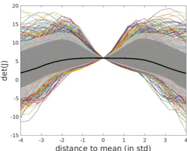
Figure 4: Determinant of the Jacobian of the mappingM :

H(1)

→ H(2)_{, as function of the distance from the mean in}

H(1)_{. On the horizontal axis, 0 refers to the location of the} mean. The plot shows an overlay of values obtained along different ‘rays’ trough the mean. The black line represents the median, while the dark and light gray areas represent the

[₋90,90]percentile region and the[₋95,95]region, respec-tively. Clearly the determinant remains positive within about a

2σ-wide area around the mean, independent of the direction.

The first experiment is chosen in line with [7, 10] and uses a CNN. It shows how convolution matrices in the first layer of a CNN show glimpses of spectro-temporal patterns similar to formant transitions. There is a similarity with the ears and noses in well-known image classification DNNs. When the number of nodes in the first hidden layer was increased from 2 to 4, 4 to 8, etc., the new convolution matrices can be seen as refining the ones in the previous run, in line with [7, 6].

The second experiment focuses on the Kullback-Leibler dissimilarity between classes in the bottleneck space as a func-tion of epoch, in which the classes are defined by the TIMIT segmentation for vowels, semivowels, liquids, nasals, fricatives, and stops. The information in the bottleneck can be considered a snapshot: during a training, classes consistently appear to their own improvement rates (with differences between classes up to a factor 4). At any time, the representation on the bottleneck may be a mix of mature and less mature unfolded acoustic struc-ture, in line with observations in [13, 8].

The third experiment shows that bottleneck representations of DNNs with the same topology trained on the same data can, in many cases, be adequately morphed into each other in a non-linear fashion. Linear mappings are insufficient for this pur-pose. This shows that bottleneck representations are actually exchangeable for other representations that look very different. It is tempting to relate this to the ‘information plane’ [8]. In our experiments we did not see hidden representations that could not be morphed, but we cannot exclude this a priori – it would imply the existence of ‘families’ or ‘regimes’ of hidden repre-sentations.

We applied small DNNs. From these experiments, which we regard as first steps, we learned that the information avail-able at the hidden layers may provide a lot of useful informa-tion, but the investigations reported here still require quite some CPU time and math machinery. Nevertheless we think informa-tion extracinforma-tion from hidden layers, also from deeper networks, is an interesting and potentially useful future direction.

5. References

[1] J. B. Tenenbaum, V. de Silva, and J. C. Langford, “A global ge-ometric framework for nonlinear dimensionality reduction,” Sci-ence, vol. 290, pp. 2319–2323, 2000.

[2] A. Jansen and P. Niyogi, “Intrinsic spectral analysis,”IEEE Trans-actions on Signal Processing, vol. 61, no. 7, pp. 1698–1710, 2013. [3] G. Marcus, “Deep Learning: A Critical Appraisal,” ArXiv

e-prints, 2018.

[4] J. Wolff, “Solutions to problems with deep learning,” ArXiv e-prints, Jan. 2018.

[5] Y. LeCun, Y. Bengio, and G. Hinton, “Deep learning,”Science, vol. 521, 2015.

[6] K. Leidal, D. Harwath, and J. Glass, “Learning modality-Invariant representations for Speech and Images,”IEEE Workshop on Au-tomatic Speech Recognition and Understanding (ASRU), 2017. [7] O. Russakovsky, J. Deng, H. Su, J. Krause, S. Satheesh, S. Ma,

Z. Huang, A. Karpathy, A. Khosla, M. Bernstein, A. C. Berg, and L. Fe, “Imagenet: Large scale visual recognition challenge,” In-ternational Journal of Computer Vision (IJCV), 2015.

[8] N. Tishby and N. Zaslavsky, “Deep learning and the information bottleneck principle,”CoRR, vol. abs/1503.02406, 2015. [Online]. Available: http://arxiv.org/abs/1503.02406

[9] G. E. Hinton and R. Salakhutdinov, “Reducing the dimensionality of data with neural networks,”Science, vol. 313, no. 5786, pp. 504–507, 2006.

[10] Y. Bengio, A. Courville, and P. Vincent, “Representation learning: A review and new perspectives,”IEEE Transactions on Pattern Analysis and Machine Intelligence, vol. 35, no. 8, pp. 1798–1828, 2013.

[11] V. Singh Tomar and R. C. Rose, “Graph based manifold regu-larized deep neural networks for automatic speech recognition,” ArXiv e-prints, Jun. 2016.

[12] R. Basri and D. W. Jacobs, “Efficient representation of low-dimensional manifolds using deep networks,” in Proceedings 5th International Conference on Learning Representations, 2017. [Online]. Available: https://openreview.net/pdf?id=BJ3filKll [13] R. Shwartz-Ziv and N. Tishby, “Opening the black box of deep

neural networks via information,”CoRR, vol. abs/1703.00810, 2017. [Online]. Available: http://arxiv.org/abs/1703.00810 [14] P. Mehta and D. J. Schwab, “An exact mapping between the

Variational Renormalization Group and Deep Learning,”ArXiv e-prints, Oct. 2014.

[15] R. Basri and D. Jacobs, “Efficient representation of low-dimensional manifolds using deep networks,”Proceedings of the International Conference on Learning Representations (ICLR), pp. 1–13, 2017.

[16] Y. Zhang, M. Pezeshki, P. Brakel, S. Zhang, C. Lau-rent, Y. Bengio, and A. C. Courville, “Towards end-to-end speech recognition with deep convolutional neural net-works,”CoRR, vol. abs/1701.02720, 2017. [Online]. Available: http://arxiv.org/abs/1701.02720

[17] M. Abadi, P. Barham, J. Chen, Z. Chen, A. Davis, J. Dean, M. Devin, S. Ghemawat, G. Irving, M. Isard, M. Kudlur, J. Levenberg, R. Monga, S. Moore, D. G. Murray, B. Steiner, P. A. Tucker, V. Vasudevan, P. Warden, M. Wicke, Y. Yu, and X. Zhang, “Tensorflow: A system for large-scale machine learning,”CoRR, vol. abs/1605.08695, 2016. [Online]. Available: http://arxiv.org/abs/1605.08695

[18] T. N. Sainath and C. Parada, “Convolutional neural networks for small-footprint keyword spotting,” inProc. Interspeech, 2015, pp. 1478 – 1482.

[19] VoiceBox. [Online]. Available: www.ee.ic.ac.uk/-hp/-staff/-dmb/-voicebox/

[20] A.-r. Mohamed, G. E. Dahl, and G. Hinton, “Acoustic modeling using deep belief networks,”IEEE Transactions on Audio, Speech, and Language Processing, vol. 20, pp. 14–22, 2012.