40, Bd. du Pont d’Arve PO Box, 1211 Geneva 4 Switzerland Tel (++4122) 312 09 61 Fax (++4122) 312 10 26 http: //www.fame.ch E-mail: [email protected]
FAME - International Center for Financial Asset Management and Engineering Matthias HAGMANN
HEC-University of Lausanne and FAME
Olivier SCAILLET
HEC-University of Geneva and FAME
Local Multiplicative
Bias Correction
for Asymmetric Kernel
Density Estimators
Research Paper N° 91 Revised October 2005
Local Multiplicative Bias Correction
for Asymmetric
Kernel Density Estimators
M. Hagmann
aO. Scaillet
bFirst version: September 2003
This version: October 2005
Abstract
We consider semiparametric asymmetric kernel density estimators when the unknown density has support on[0,∞). We provide a unifying framework which relies on a local multiplicative bias correction, and contains asymmetric kernel versions of several semiparametric density estimators considered previously in the literature. This framework allows us to use popular parametric models in a nonparametric fashion and yields estimators which are robust to misspecification. We further develop a specification test to determine if a density belongs to a particular parametric family. The proposed estimators outperform rival non- and semiparametric estimators in finite samples and are easy to implement. We provide applications to loss data from a large Swiss health insurer and Brazilian income data.
Key words and phrases: semiparametric density estimation, asymmetric kernel, income distribution, loss distribution, health insurance, specification testing.
JEL Classification: C13, C14.
a HEC Lausanne and FAME, 33 Route de Chavannes, CH-1007 Lausanne.
E-mail: [email protected].
b HEC Genève and FAME, UNIMAIL, 102 Bd Carl Vogt, CH-1211 Genève.
1
Introduction
One of the major concerns of insurance companies is the study of a group of risks. For insurers, a good understanding of the size of a single claim is of most importance. Loss distributions describe the probability distribution of a payment to the insured. Traditional methods in the actuarial literature use parametric specifications to model single claims. The most popular specifications are the lognormal, Weibull and Pareto distributions. Hogg and Klugman (1984) and Klugman, Panjer and Willmot (1998) describe a set of continuous parametric distributions which can be used for modelling a single claim size. It is, however, unlikely that something as complex as the generating process of insurance claims can be described by just a few parameters. A wrong parametric specification may lead to an inadequate measurement of the risk contained in the insurance portfolio and consequently to a mispricing of
insur-ance contracts. These remarks also apply to financial losses, portfolio selection and risk management
procedures in a banking context.
In a totally different area of research, economists studying income distributions and income inequality use similar parametric models to estimate the distribution of income and its evolution over time. Popular models are the gamma, lognormal and Pareto distributions, see Cowell (1999). Whereas the lognormal distribution is thought to have the best overall shape, the Pareto is considered to be a more suitable distribution for individuals in the upper end of the income distribution. Although these densities may capture some stylised facts of income distributions, it is again unlikely that income distributions can be described by just a few parameters. The imposition of a wrong parametric model may lead to inconsistent estimates and misleading inference, as well as to disputable conclusions in inequality measurement for example.
A method which does not require the specification of a parametric model is nonparametric kernel smoothing. This method provides valid inference under a much broader class of structures than those imposed by parametric models. Unfortunately, this robustness comes at a price. The convergence rate of nonparametric estimators is slower than the parametric rate, and the bias induced by the smoothing procedure can be substantial even for moderate sample sizes. Since both income and losses are positive variables, the standard kernel estimator proposed by Rosenblatt (1956) has a boundary bias. This
boundary bias is due to weight allocation by the fixed symmetric kernel outside the support of the
distribution when smoothing close to the boundary is carried out. As a result, the mode close to the boundary typical for income and loss distributions is often missed. Additionally, standard kernel methods yield wiggly estimation in the tail of the distribution since the mitigation of the boundary bias leads to favour a small bandwidth which prevents pooling enough data. Precise tail measurement of loss distributions is however of particular importance to get appropriate risk measures when designing an efficient risk management system.
We propose a semiparametric estimation framework for the estimation of densities which have sup-port on [0,∞). Our estimation procedure can deal with all problems of the standard kernel estimator mentioned previously, and this in a single way. Although the above parametric models may be inaccu-rate, they can be used in a nonparametric fashion to help to decrease the bias induced by nonparametric smoothing. If the parametric model is accurate, the performance of our semiparametric estimator can be close to pure parametric estimation. Following Hjort and Glad (1995) (H&G), we start with a para-metric estimator of the unknown density (economic theory may help in providing the parapara-metric start), and then correct nonparametrically for possible misspecification. To decrease the bias even further, we give some local parametric guidance to this nonparametric correction in the spirit of Hjort and Jones (1996) (H&J). This is achieved by employing either local polynomial or log polynomial models,
where the latter method results always in nonnegative density estimates. We call this approach local
multiplicative bias correction, or LMBC to be short.
We emphasize that appropriate boundary bias correction is more important in a semiparametric than a pure nonparametric setting. This is because the bias reduction achieved by semiparametric techniques allows us to increase the bandwidth and thus to pool more data. This, however, increases the boundary region where the symmetric kernel allocates weight to the negative part of the real line. This motivates us to develop LMBC in an asymmetric kernel framework which eliminates the
boundary issue completely1. Asymmetric kernel estimators were recently proposed by Chen (2000)
as a convenient way to solve the boundary bias problem. The symmetric kernel is replaced by an
asymmetric gamma kernel which matches the support of the unknown density2. As an alternative
to the gamma kernel, Scaillet (2004) introduced kernels based on the inverse Gaussian and reciprocal inverse Gaussian density. All of these kernel functions haveflexible form, are located on the nonnegative real line and produce nonnegative density estimates. Also, they change the amount of smoothing in a natural way as one moves away from the boundary. This is particularly attractive when estimating densities which have areas sparse in data because more data points can be pooled. As pointed out by Cowell (1999) ”Empirical income distributions typically have long tails with sparse data”. The same holds true for empirical loss distributions and we therefore think that these kernels are very well suited in this context. The variance advantage of the asymmetric kernel comes, however, at the cost of a slightly increased bias as one moves away from the boundary compared to symmetric kernels, which highlights the importance of effective bias reduction techniques in the tails. In a comprehensive
1The theoretical results derived in this paper show that the form of the bias reduction achieved through LMBC is analogous in the symmetric and asymmetric kernel case, although the mathematics and the strategy of the proof yielding these results are totally different. Obviously we cannot exploit symmetry in the derivation of the results for asymmetric kernels.
2Other remedies include the use of particular boundary kernels or bandwidths, see e.g. Rice (1984), Schuster (1985), Jones (1993), Müller (1991) and Jones and Foster (1996).
simulation study, Scaillet (2004) obtains attractivefinite sample performance of these asymmetric kernel estimators. He also reports that boundary kernel estimators lead too often to negative density estimates without outperforming asymmetric kernel density estimators. Chen (2000) reports superior performance of the gamma kernel estimator compared to other remedies proposed in the literature as the local linear estimator of Jones (1993). A particular advantage of the gamma kernel estimator is its consistency when the true density is unbounded atx= 0, which is important for the estimation of highly skewed loss and income distributions. This is shown in Bouezmarni and Scaillet (2005) who also establish uniform and
L1 convergence results for asymmetric kernel density estimators. Furthermore they report nice finite
sample performance of the asymmetric kernel density estimator w.r.t. the L1 norm.
Our simulation study underlines the importance of efficient boundary correction in a semiparametric
framework. We find that LMBC in connection with asymmetric kernels yields excellent results. These
estimators perform better in a mean integrated squared error (MISE) sense than pure nonparametric estimators. If the parametric information provided is accurate, wefind that a MISE reduction of 50-80% can be reasonably expected. Even if the misspecification considered is large, our LMBC estimator still achieves a MISE reduction of around 25%. Asymmetric kernel based LMBC estimators outperform their symmetric rivals: first because they eliminate the boundary bias issue more successfully (allowing a larger bandwidth), and second because they have an intrinsic advantage in the tails of the density. Furthermore, they are often easier to implement.
As a by-product of our approach, we propose a new attractive semiparametric specification test to determine whether a particular unknown density belongs to a parametric class of densities. The test is very simple to implement and should prove useful in empirical applications. We also explain how this statistic can be used to determine which density can be felt as a suitable parametric start.
Although we concentrate in the empirical part on loss and income distributions, similar issues as
discussed above are also important in the finance literature. Aït-Sahalia (1996a) develops an
estima-tion procedure for diffusion models of the short term interest rate. Based on Bickel and Rosenblatt’s (1973) work on density matching, Aït-Sahalia (1996b) also proposes a way to test various parametric specifications for diffusion models of the short rate. In his estimation and specification framework, the nonparametric estimation of the stationary distribution of the interest rate process plays a key role. The intertemporal general equilibrium asset pricing model of Cox, Ingersoll and Ross (1985) implies that this distribution follows a gamma probability law. Although this interest rate model may again be overly restrictive, it gives some economic guidance about the likely form of the stationary distribution of the short rate. This information can be incorporated in a semiparametric estimator like ours. Fur-thermore, our results are potentially important for estimation and specification testing of the baseline
hazard function in financial duration analysis. In this literature parametric models like the Burr and
(2000) for an overview of autoregressive conditional duration models (ACD), Tyurin (2003) for a recent application of the competing risk model to the foreign exchange market, and Fernandes and Grammig (2005) for exploitation of asymmetric kernels in financial duration analysis. Clearly the standard ker-nel estimator is again not appropriate in these contexts, since it does not take into account that the underlying variables, interest rates and durations, are nonnegative.
The outline of the paper is as follows. In Section 2 we introduce our semiparametric estimation framework and relate it to the relevant associated literature. This unified framework embeds semipara-metric density estimators developed by H&G, H&J, and Loader (1996), and allows us to fully clarify the interdependence between these approaches. Section 3 recalls asymmetric kernel methods. Section 4 contains the main contribution of the paper, namely the extension of the LMBC framework to the asymmetric kernel case. We develop several examples, which show that the estimation procedure is user
friendly and remarkably simple to implement in most cases3. The procedure is therefore appealing for
applied work. We also discuss bandwidth choice and model diagnostic tests. In Section 5 we compare the performance of our estimators through an extensive simulation study. To the best of our knowledge,
it is the first time that the various semiparametric approaches mentioned above are compared on a
finite sample basis. In Section 6 we provide two empirical applications: thefirst one to loss data from a large Swiss health insurer, the second one to Brazilian income data. Section 7 contains some concluding remarks. An appendix gathers the proofs and technicalities related to the properties of the various estimators considered in the text.
2
Local multiplicative bias correction
In nonparametric regression, local polynomial fitting is a very popular approach, e.g. Fan and Gijbels
(1996) and the references therein. Gozalo and Linton (2000) are the first to consider local fitting of a general functional using a least squares criterion, a normal error distribution version of a local likelihood estimator. For density estimation, the local likelihood approach was independently developed at the same time by H&J and Loader (1996). For a recent extension of the approach with application to Value-at-Risk (VaR) in risk management, see Gourieroux and Jasiak (2001). Whereas Loader (1996) concentrates on local polynomial fitting to the logarithm of the density, H&J allow for general local functionals like Gozalo and Linton (2000) in regression estimation.
In this section, we briefly introduce an estimation framework based on familiar symmetric kernel methods, which contains as special cases the local likelihood and multiplicative bias correction approach as described in H&J, Loader (1996), and H&G, respectively. This framework will allow us to derive the
properties of these methods using asymmetric kernels in a single step, instead of treating the methods separately. Furthermore it allows us to shed some light on the intertwinning of these methods.
Let X1, ..., Xn be a random sample from a probability distribution F with an unknown density
function f(x) where x has support on [0,∞). We propose the following local model as a basis to
estimate the true density function f(x):
m(x, θ1, θ2(x)) =f(x, θ1)r(x, θ2(x)). (2.1)
Thefirst part of the local modelmconsists off(x, θ1), which is a parametric family of densities indexed
by the global parameterθ1 = (θ11, ..., θ1p)∈Θ1 ∈Rp.This term serves as a global parametric start and
is assumed to provide a meaningful but potentially inaccurate description of the true densityf(x). The second part ofmdenoted byr(x, θ2(x))with θ2(x) = (θ21(x), ..., θ2q(x))∈Θ2 ∈Rq serves as the local
parametric model for the unknown function r(x) =f(x)/f(x, θ1). The role of this ’correction function’
is, as the name says, to correct the potentially misspecified global start densityf(x, θ1)towards the true
density f(x). H&J briefly discuss this local model as a particular example in their paper, whereas we use it to provide a general framework for several semiparametric estimators proposed in the literature. We call this local multiplicative bias correction (LMBC) since only the multiplicative correction factor is modelled locally. Note that the correction function r(x) is uniformly equal to one if the parametric start is well specified. Hence when the degree of misspecification is not too severe it is intuitively more natural to model the correction factor locally than the unknown density itself.
The procedure is as follows: first, estimate the parameter θ1, which does not depend on x, by
maximum likelihood. It is well known that when the parametric model f(x, θ1) is misspecified, θ1
converges in probability to the pseudo true value θ01 which minimizes the Kullback-Leibler distance
of f(x, θ1) from the true f(x), see e.g. White (1982) and Gourieroux, Monfort and Trognon (1984).
Second, choose θ2(x)such that
1 n n X i=1 Kh(Xi−x)v(x, Xi, θ2)− Z Kh(t−x)v(x, t, θ2)f ³ t,ˆθ1 ´ r(t, θ2)dt= 0 (2.2)
holds, where Kh(z) = (1/h)K(z/h) is a symmetric kernel function, h is the bandwidth parameter and v(x, t, θ2) is a q×1 vector of weighting functions. We omit for notational simplicity the possible
dependence of the weighting function on θ1. If we choose the score ∂logm(x, θ1, θ2(x))/∂θ2 as the
weighting function, then Equation (2.2) is just the first order condition of the local likelihood function given in H&J. In general, the form of the weighting function is driven by the tractability of the implied resulting estimator and is discussed in more detail as we proceed in the paper. The local multiplicatively bias corrected density estimator is
ˆ f(x) =f³x,ˆθ1 ´ r³x,ˆθ2(x) ´ . (2.3)
From the theoretical results concerning bias and variance of the local likelihood estimator given in H&J, it immediately follows that this estimator has the same variance as the standard kernel density estimator introduced by Rosenblatt (1956). The bias is however different. Compared to H&J, we prefer to state the bias in terms of the correction factor. This is more intuitive and simplifies the comparison between different estimation strategies. To ease notation, we writef0(x) =f
¡
x, θ01¢andr0(x) =f(x)/f
¡ x, θ01¢. Whenθ2 is one dimensional, the bias is4
Bias³fˆ(x)´ = σ2Kh2 µ 1 2f0(x) h r0(2)(x)−r(2)(x, θ02)i (2.4) +{v (1) 0 (x) v0(x) f0(x) +f (1) 0 (x)} h r(1)0 (x)−r(1)(x, θ02)i ! ,
where σ2K = R z2K(z)dz and v0(x) denotes v(x, x, θ02). The magnitude of this bias term depends on
how well the correction function can be approximated locally by a suitable parametric model. This is so if r(x) is smooth, or equivalently, if the global parametric start is close to the true density. In the single parameter case, the bias also depends on the weighting function and on the distance between the slopes of the correction function and its local model. If dim (θ2)≥ 2, the bias is free of this term and
only the first term in the brackets appears. For further details we refer to H&J.
Direct local modelling of the density can be obtained by choosing the parametric start density as an improper uniform distribution. W.l.o.g. set f0(x)to one. Then the only source of bias reduction is
provided by the local model r(x, θ). The bias is 12σ2
Kh2 h r0(2)(x)−r(2)(x, θ0 2) i as in H&J.
The multiplicatively corrected kernel estimator of H&G emerges from choosing the weighting function as 1/f³x,ˆθ1
´
, and choosing the local model as a constant. From Equations (2.2) and(2.3) it follows that the estimator is
ˆ f(x) = f ³ x,ˆθ1 ´ R Kh(t−x)dt 1 n n X i=1 Kh(Xi−x) 1 f³Xi,ˆθ1 ´. (2.5)
From(2.4), the bias is(1/2)σ2
Kh2f0(x)r(2)(x), which is the bias obtained by H&G and does not depend
on the chosen weighting function. We remark that this is the only possible choice of weighting function which sets the second bracket term in Equation (2.4) to zero. Assuming that K has support [−1,1]5, the term in the denominator of Equation (2.5) integrates to one if x lies in the interior, meaning that
x/h → κ > 1. However, close to the boundary where 0 ≤ κ < 1, this integral term normalizes the density estimate and therefore adjusts for the undesirable weight allocation of the symmetric kernel
4Sinceˆθ
1 exhibits √n-convergence which is faster than the nonparametric rate, the additional variability introduced
through thefirst step estimation ofθ1does not influence the bias and variance offˆ(x)up to negligible higher order terms.
5This setup can easily be extended to infinite support kernels. However, finite support is a standard assumption, delineating boundary and interior regions.
outside the support of the density. This adjustment is not optimal and boundary bias is still of the undesirable order O(h). Like in nonparametric regression, see e.g. Fan and Gijbels (1992), one of the possible boundary bias correction methods which achieves an O(h2) order is the popular local linear estimator, see Jones (1993) for the density case. To obtain a local linear H&G version we propose to choose the local model as r(t, θ2) = θ21 +θ22(t−x) and the weight functions as 1/f(t, θ1) and
(t−x)/f(t, θ1). The resulting estimator is equivalent to the H&G estimator in the interior of the
density. Close to the boundary it provides however again a correction due to weight allocation of the symmetric kernel to the negative part of the real line. Define αj(κ) =
Rκ
−1K(u)u
jdu, then the local linear estimator in the boundary region is
ˆ f(x) =f ³ x,ˆθ1 ´rˆ(x)−[α1(κ)/hα2(κ)] ˆg(x) ¡ α0(κ)−α1(κ)2/α2(κ) ¢ , (2.6)
where ˆg(x)is the sample average of Kh(Xi−x)
h (Xi−x)/f ³ Xi,ˆθ1 ´i .
After presenting this unifying framework for previously proposed estimators, we now turn to an asymmetric kernel version of the above approach. Since the support of these kernels matches the support of the density under consideration, no boundary correction of the type presented above is necessary by construction. Wefirst briefly review asymmetric kernel estimators for densities defined on the nonnegative real line introduced by Chen (2000) and Scaillet (2004). In Section 4 we will treat the LMBC case.
3
Asymmetric kernel methods
The asymmetric kernel density estimator is
ˆ fb(x) = 1 n n X i=1 K(Xi;x, b), (3.1)
where bis a smoothing parameter satisfyingb→0 andbn→ ∞ asn→ ∞. The asymmetric weighting
function K is either a gamma density KG with parameters(x/b+ 1, b)as proposed by Chen (2000), an inverse Gaussian density KIG with parameters (x,1/b), or a reciprocal inverse Gaussian density KRIG with parameters (1/(x−b),1/b) as proposed by Scaillet (2004). These kernel densities are
KG(t; x b + 1, b) = tx/bexp (−t/b) Γ(x/b+ 1)bx/b+1, KIG(t;x, 1 b) = 1 √ 2πbt3 exp µ − 1 2bx µ t x −2 + x t ¶¶ , KRIG(t; 1 x−b, 1 b) = 1 √ 2πbtexp µ −x−b 2b µ t x−b−2 + x−b t ¶¶ .
Note that these asymmetric kernels do not take the formω(x−t, b)whereω is an asymmetric function (instead of a symmetric one), and thus do not belong to the class of asymmetric kernels studied by
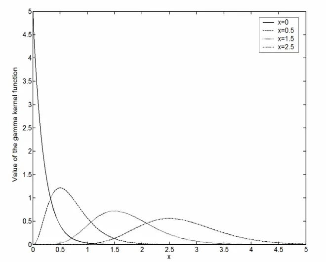
Abadir and Lawford (2004). Figure 1 displays the gamma kernel for some selected x-values. All
asymmetric kernels share the property that the shape of the kernel changes according to the value of x. This varying kernel shape changes the amount of smoothing applied by the asymmetric kernel since the variance of, for instance, KG(t;xb + 1, b) is xb+b2, which is increasing in x as we move away from the boundary. This is also reflected in the bias and variance expressions, which we give here for the gamma kernel estimator, and on which we concentrate below:
Bias³fˆbG(x)´ = ½ f(1)(x) +1 2xf (2)(x) ¾ b+o(b), (3.2) Var³fˆbG(x) ´ = ( 1 2√πn− 1b−1/2x−1/2f(x) if x/b → ∞, Γ(2κ+1) 21+2κΓ2(κ+1)n−1b−1f(x) if x/b→κ.
This estimator is not subject to boundary bias, but involves thefirst derivative of the unknown density. This is becausexis not the mean of the gamma kernelKG(t;xb+ 1, b), rather its mode. This is different for the inverse Gaussian and reciprocal inverse Gaussian kernel estimators, whose biases only involve the second order derivative of the unknown density. To circumvent thefirst derivative in the bias expression, Chen (2000) also proposes a second gamma kernel which is, as Scaillet (2004) reports, similar in shape as the reciprocal inverse Gaussian kernel but has a slightly inferior finite sample performance.
Compared to other boundary correction techniques, the bias of gamma kernel estimators may be larger asxincreases, this is however compensated by a reduced variance. In the interior wherex/b→ ∞, it is apparent from(3.2)that the variance of the gamma kernel estimator decreases asxgets larger. This is in contrast to symmetric kernel estimators whose variance coefficients remain constant outside the boundary area. Also asymmetric kernels have a larger effective sample size than kernels with compact support. This is desirable for estimating densities with sparse areas as more data points can be pooled. In the following we address the question of semiparametric bias reduction techniques for asymmetric kernel methods. This is important since as just reported, the bias may be larger than for standard symmetric kernel methods. Effective bias reduction techniques combined with a variance decreasing as we move away from the boundary is giving us hope for promising performance of our estimators for the estimation of loss and income distributions. This will be confirmed later in the paper.
4
Local multiplicative bias correction with asymmetric
ker-nels
Apart from being an attractive semiparametric bias reduction framework, LMBC allows us to implement a popular boundary bias reduction by choosing a local linear model for the density or correction factor.
This boundary bias reduction is not necessary per se in the asymmetric kernel framework since no
weight is allocated outside the support of the unknown density. The effect of LMBC in an asymmetric framework is just to reduce the potentially larger bias for asymmetric kernel techniques. In addition, LMBC in connection with asymmetric kernels allows for the construction of user friendly estimators despite the apparent complexity of the approach. Estimators based on symmetric kernels, like e.g. the Gaussian kernel, often require numerical integration and optimization procedures. Bolancé et. al. (2003) mention that nonparametric methods for loss distribution estimation are seldom applied in practice because of implementation difficulties. Candidate estimators must be easy to implement to have a chance of being applied in the non-academic world. Numerical tractability is also a key advantage when resampling methods such as the bootstrap are used for inferential purposes.
We now extend the LMBC approach to the asymmetric kernel case, compute bias and variance of the estimator and discuss the choice of bandwidth. We also consider the special cases of H&J, Loader (1996), and H&G, and show how these methods can be applied to the estimation of income and loss distributions.
4.1
De
fi
nition of the estimator
We follow the notation introduced in Section 2. The estimator is f˜b(x) =f
³ x,ˆθ1 ´ r³x,ˆθ2(x) ´ , where ˆ
θ1 is the global maximum likelihood estimator which does not depend on x, and ˆθ2(x) is chosen by
maximizing the local likelihood function
logLn ³ x,ˆθ1, θ2 ´ = Z ∞ 0 K(t;x, b){logm³t,ˆθ1, θ2 ´ dFn(t)−m ³ t,ˆθ1, θ2 ´ dt} = 1 n n X i=1 K(Xi;x, b) logm(Xi,ˆθ1, θ2)− Z ∞ 0 K(t;x, b)m(t,ˆθ1, θ2)dt, (4.1)
with Fn denoting the empirical distribution function. This criterion function is equivalent to the one of H&J. However, the symmetric kernel is replaced by an asymmetric kernel, whose support matches the support of the density we wish to estimate. For notational simplicity we omit the local dependency of θ2 on x. The first term in (4.1) is the standard log-likelihood function weighted by an asymmetric
kernel function. Maximizing this term alone would lead to inconsistent results because the expectation of its score is not equal to zero at the true parameter value θ02.The second term guarantees that this is
the case; we refer to H&J. From(4.1), whenbis very large, K(t;x, b) is independent oft and the above expression is a constant times the ordinary, normalized log-likelihood function. The maximization of
the local likelihood then becomes the same as ordinary likelihood maximization. But if b is small, the
maximization oflogLn
³
x,ˆθ1, θ2
´
will provide the best local estimator off(x). This follows since under some regularity conditions,
logLn ³ x,ˆθ1, θ2 ´ p →π(x, θ01, θ2) = Z ∞ 0 K(t;x, b){f(t) logm(t, θ10, θ2)−m(t, θ01, θ2)}dt,
as n grows. Hence ˆθ2, the maximizer of (4.1), aims at the parameter value θ02(x) that maximizes
π(x, θ01, θ2) when the above convergence is uniform over the parameter space. See for example Linton
and Pakes (2001). The solution to the above problem minimizes the following distance measure which is a localized version of the Kullback-Leibler distance of f(x)from m(x, θ01, θ2):
d[f, m(·, θ01, θ2)] = Z ∞ 0 K(t;x, b) ∙ f(t) log f(t) m(t, θ01, θ2) −{ f(t)−m(t, θ01, θ2)} ¸ dt.
This shows that ˆθ2 aims at the best local parametric approximant to the true f. The estimator
de-pends on the chosen smoothing parameter. For further details and justifications of the local likelihood approach, see H&J, Loader (1996), and the references therein.
The estimator ˆθ2 for general weight functions v(x, t, θ2)is defined to be the solution to
Vn ³ x,ˆθ1, θ2 ´ = 1 n n X i=1 K(Xi;x, b)v(x, Xi, θ2)− Z ∞ 0 K(t;x, b)v(x, t, θ2)m(t,ˆθ1, θ2)dt = 0. (4.2)
This is identical to thefirst order condition of(4.1)in the case wherev is chosen as the scoreu(t, θ2) =
(∂/∂θ2) logr(t, θ2). For identification reasons, assume that
Vn ³ x,ˆθ1, θ2 ´ p →V ¡x, θ01, θ2 ¢ = Z K(t;x, b)v(x, t, θ2)f0(x){r0(t)−r(t, θ2)}dt= 0
has a unique solution atθ2 =θ02. This requires that theqweight functions are functionally independent,
and that the correction functionr0(t)is within reach of the parametric modelr(t, θ2)asθ2 varies. This
is like M-estimation in a possibly misspecified case, since the true correction function does not have to belong to the parametric familyr(t, θ).
4.2
Large sample properties
We now develop the bias and variance of the LMBC estimator. The derivations of all results presented here are given in the appendix. When not stated otherwise, we will focus on results for the gamma kernel developed in Chen (2000) since other kernel choices can be handled in a similar fashion.
If we locally fit one parameter, the bias of the LMBC estimator is Bias³f˜bG(x)´ = f0(x) ∙ {r(1)0 (x)−r(1)(x, θ02)}+ 1 2x{r (2) 0 (x)−r (2)(x, θ0 2)} ¸ b + Ã v0(1)(x) v0(x) f0(x) +f0(1)(x) ! x{r0(1)(x)−r (1) (x, θ02)}b +o(b) +O µ 1 nb1/2 ¶ , (4.3)
where we use the same notation as in the second section of this paper. H&J also note that the first derivative will vanish automatically from the bias expression if the numberqof locallyfitted parameters is larger than two. Equation (4.3) will then hold for any component vj,0(x) of the weighting function,
which can only be true ifhr(1)0 (x)−r(1)(x, θ0 2)
i
=o(1)asb→0. This is not generally the case with one parameter. This means that for q≥2, the bias reduces to
Bias³f˜bG(x)´= 1 2f0(x){r (2) 0 (x)−r (2)(x, θ0 2)}xb+o(b) +O µ 1 nb1/2 ¶ . (4.4)
H&J show that for q ≥ 3 one can argue that {r0(2)(x)−r(2)(x, θ 0
2)} is also o(1) and third and fourth
order derivatives appear in the bias term. This property also holds for asymmetric kernels. We also
note that Chen (2002) introduced a local linear regression estimator based on the first gamma kernel,
which has thefirst derivative removed from the bias expression compared to the standard local constant regression smoother.
There are several worthwhile remarks. First, we obtain the same result as in the symmetric kernel case albeit relying on different proof techniques adapted to our asymmetric framework. Comparing Equations (3.2) and (4.4), the first derivative vanished and the second derivative in the bias of the asymmetric kernel estimator is replaced by f0(x)
h
r(2)0 (x)−r(2)(x, θ0 2)
i
. So this estimator performs better than pure asymmetric kernel methods if the latter expression is smaller than the former in absolute values. This is the case if the unknown density exhibits high local curvature or if the parametric start is close to the true density since then r(2)0 (x) is small. Additionally, the local model for the correction
factor can make this term even smaller if it can locally capture the curvature of the correction factor. If the model is correct, the local likelihood estimator is unbiased up to the order considered.
The variance of the asymmetric LMBC estimator in the one parameter case is Var³f˜bG(x)´= ( 1 2√πn− 1b−1/2x−1/2f(x) if x/b → ∞, Γ(2κ+1) 21+2κΓ2(κ+1)n− 1b−1f(x) if x/b →κ, (4.5)
where κ is a positive constant. We therefore obtain exactly the same result for the variance as for
depend on the chosen weighting functions. We therefore have some flexibility to select them to obtain estimators which are tractable to implement.
The variance of the LMBC estimator in the multiple parameter case for a general asymmetric kernel is Var³f˜(x)´= f(x) n e t 1τ(K)e1− f(x)2 n +O(b/n), (4.6)
where, using some simplified notation, τ(K) is given by
µZ ∞ 0 K(t)VtV 0 tdt ¶−1µZ ∞ 0 K(t)2VtV 0 tdt ¶ µZ ∞ 0 K(t)VtV 0 tdt ¶−1
and Vt is q × 1 vector containing in the jth position the elements (t−x) j−1
for j = 1, ..., q. This expression depends on the kernel being used. Independent of the kernel used, the variance of the LMBC estimator in the two parameter case is the same as in the single parameter case. We collect results for all the asymmetric kernel estimators in the following proposition.
Proposition 1 The bias expressions of the asymmetric LMBC estimator in the cases where K is the gamma, inverse Gaussian and reciprocal inverse Gaussian kernel are given for q≥2 by:
Bias³f˜bG(x) ´ = 1 2xf0(x) h r(2)0 (x)−r (2) (x, θ02) i b+o(b), Bias³f˜bIG(x)´ = 1 2x 3f 0(x) h r0(2)(x)−r(2)(x, θ02)ib+o(b), Bias³f˜bRIG(x)´ = 1 2xf0(x) h r(2)0 (x)−r(2)(x, θ02)ib+o(b).
The variances of the asymmetric LMBC kernel estimator are the same as those in the pure nonpara-metric case.
Note that global performance measures such as MISE are easy to derive from these results (see Section 4.5).
4.3
Special cases
After developing the general LMBC framework, properties of special cases are now derived. As described in Section 2, direct local modelling of the density can be obtained by choosing the parametric start den-sity as an improper uniform distribution. W.l.o.g. we can set f0(x) to one. The local model r(t, θ) is
then the only source of bias reduction. As soon as we fit two or more local parameters(q≥2), Propo-sition 1 implies that the bias of the asymmetric local likelihood estimator is 12xahr(2)
0 (x)−r(2)(x, θ 0 2)
i b,
where a is equal to three for the inverse Gaussian and one for the other asymmetric kernels. The
the weighting function as1/f³t,ˆθ1
´
and choosing the local model as a constant. From Equation(4.2)
it follows that the estimator is in this case
˜ fb(x) =f(x,ˆθ1)ˆr(x) = 1 n n X i=1 K(Xi;x, b) f(x,ˆθ1) f(Xi,ˆθ1) .
This estimator has the advantage that it is very simple to implement. Chen’s asymmetric kernel estimator has therefore an implicit initial parametric start which is given by an improper uniform distribution. The ratio f(x,ˆθ1)/f(Xi,ˆθ1) equals one in this case. This time, no boundary correction
terms are needed which contrasts with symmetric kernels. This is because the asymmetric kernel already answers the boundary bias issue. An estimation technique closely related to H&G is the multiplicative
bias correction approach developed by Jones, Linton and Nielsen (1995) (JLN)6. The analogue of their
estimator for asymmetric kernels is
¯ f(x) = ˆfb(x)ˆα(x) = 1 n n X i=1 K(Xi;x, b) ˆ fb(x) ˆ fb(Xi) ,
where fˆb(x) is the usual asymmetric kernel estimator given in Equation (3.1). For symmetric kernels, this estimator has generally a smaller bias than the standard kernel estimator at the cost of a slightly larger variance. We do not further pursue this idea here since the JLN bias correction procedure is fully nonparametric. It should be possible to derive properties of this estimator in the asymmetric case combining techniques given in JLN and Chen (2000).
4.4
Examples
After developing the general framework, we now show how this framework can be applied to the esti-mation of densities with support on the nonnegative real line. We focus especially on examples which are relevant for the estimation of loss and income distributions. We give examples for the asymmetric LMBC and the asymmetric version of the H&G estimator, and also explore the case where the local model is chosen to fit the density directly as in H&J and Loader (1996).
4.4.1 A gamma start
A parametric start which is sufficiently flexible and can be expected to be appropriate in applications
for unimodal and right skewed distributions is given by the gamma density7. This parametric start can
6This estimator can be obtained by choosing a nonparametric start estimator and choosing 1/fˆ
b(x) instead of 1/fb
³ x,ˆθ1
´
as the weighting function. However, this time thefirst estimation step does influence the variance of thefinal estimator, and therefore we can not embed this estimator in the LMBC framework.
7An example based on the gamma (and also log-normal) density using symmetric kernels can be found in H&G. Their estimator suffers, however, from boundary bias like standard kernel estimators.
be combined with a local polynomial model for the correction factor: r(t, θ2) =θ21+θ22(t−x) +...+ θ2(q+1)(t−x)q. The estimator is f˜b(x) = f ³ x,ˆθ1 ´ ˆ
θ21(x). The gamma start density in combination
with the gamma kernel yields easy to implement estimators, which is a further advantage of our method and obviously of considerable importance for practical empirical investigations.
Example 1 Using the above model for the correction factor, choosing the weight functions(t−x)j for
j = 0, ..., qand using Equation(4.2),one can easily establish that the semiparametric density estimator
with a gamma start fG
³
x,α,ˆ βˆ´ for a general orderq is
˜ fb(x, q) =fG ³ x,α,ˆ βˆ´et1 ⎡ ⎢ ⎢ ⎣ δ0 ... δq ... ... ... δq ... δ2q ⎤ ⎥ ⎥ ⎦ −1⎡ ⎢ ⎢ ⎣ ˆ f0 b (x) ... ˆ fbq(x) ⎤ ⎥ ⎥ ⎦, where δj = Z ∞ 0 KG à t;x/b+ ˆα, b βˆ ˆ β+b ! (t−x)jdt, c = Γ¡xb + ˆα¢ ³bβˆβ+ˆb´ x/b+ˆα Γ(ˆα) ˆβαˆΓ(x/b+ 1)bx/b+1 , (4.7)
andfˆbj(x)is the sample average of(Xi−x) j
KG
¡
Xi;xb + 1, b
¢
. Choosing the local model as a constant is not particularly attractive since the bias of this estimator contains also the first order derivative of
the correction function and the local model. These first derivative terms vanish if we choose a local
polynomial model for the correction factor with q ≥ 2. In particular, the local linear version of this estimator has the same bias as the asymmetric H&G estimator if K is chosen as the RIG or IG kernel:
˜ fb(x) = 1 n n X i=1 K(Xi;x, b) µ x Xi ¶αˆ−1 expn−βˆ(x−Xi) o . (4.8)
Both estimators are attractive when the true density is close to the gamma family. Otherwise a local model for the correction factor is desirable to capture curvature and further diminishes the bias. This
can be attained by choosing q ≥ 3. We will consider the gamma kernel version of the estimator in
Equation (4.8) in our simulation study and will refer to it as the AHGG estimator.
Example 2 An alternative to local polynomial modelling of the correction factor isfitting a polynomial to the logarithm of the correction factor, choosingr(t, θ2) =θ21exp
¡
θ22(t−x) +...+θ2(q+1)(t−x)
q¢
.
Compared to direct polynomialfitting as described above, this ensures a positive estimator and promises a better performance than the H&G estimator if the true density is not given by the parametric start8.
8Note from(4.4)that the leading term of the bias of this estimator is given by1
2f0(x){r (2)
0 (x)−r(2)(x, θ 0
2)}xbcompared
We work out below the local log linear version of this estimator with a gamma start, again using the
gamma kernel. Using Equation (4.2) and the score as the weighting function, the equation system to
be solved is ˆ fb(x) = cθ21exp (−θ22x)ψ(θ22), (4.9) ˆ fb1(x) = cθ21exp (−θ22x) h ψ(1)(θ22)−xψ(θ22) i , (4.10)
where ψ(θ22) is the moment generating function associated with KG
³
t;x/b+ ˆα, bˆββ+ˆb´ and c is as defined in (4.7). This function is9
ψ(θ22) = (1−β∗θ22)−α ∗
for θ22≤β∗−1,
where α∗ =x/b+ ˆα, β∗ =bβˆ+βˆb. Since f˜b(x) =fG
³
x,α,ˆ βˆ´ˆθ21, ˆθ22 is only somewhat "silently" present
in the local parameterization. Using this and Equations (4.9)and (4.10)one obtains
ˆ
θ22 =
(q+x)−α∗β∗
β∗(q+x) , (4.11)
whereq = ˆf1
b(x)/fˆb(x). From(4.9), we can then obtain a closed form expression for the LMBC estimator with a gamma start and the log linear correction factor
˜ fb(x) =fG ³ x,α,ˆ βˆ´ fˆb(x) cexp³−ˆθ22x ´ ψ³ˆθ22 ´. (4.12)
So with a gamma start this estimator is clearly simple to implement and should reveal appropriate in
many circumstances because of the shape flexibility of the gamma distribution. We will refer in the
Monte Carlo Section to the estimator of Equation (4.12) as the ALMBC estimator.Unfortunately this
simplicity does not extend to other parametric starts than the gamma density. There the integrals corresponding to those in Equation (4.2) have to be calculated numerically.
4.4.2 Lognormal and Weibull start
Whereas the integral in Equation (4.2) can be analytically evaluated when we use a gamma kernel in
combination with a gamma start, this is no longer true for other popular densities which have support on the nonnegative real line. There, numerical integration techniques are required. It is therefore convenient to choose the H&G weight function which automatically solves this problem. This simplicity of the H&G estimator makes this approach particularly attractive. We develop here two examples based on parametric start densities which are used in the literature for income and loss distribution modelling. We follow the notation of Klugman et al. (1998).
9It can easily be checked that the solutionˆθ
Example 3 One popular parametric model for loss and income distributions is given by the lognormal probability law LN(μ, σ). This parametric model is usually thought as the best overall choice to fit loss data. The asymmetric H&G estimator is
˜ fb(x) = 1 n n X i=1 K(Xi;x, b) exp©−12(logx−μˆ)2/σˆ2ª exp©−1 2(logXi−μˆ) 2 /σˆ2ª Xi x .
Example 4 Another useful parametric start is the Weibull W(θ, τ) probability law. The exponential density results if τ = 1. We have then:
˜ fb(x) = 1 n n X i=1 K(Xi;x, b) µ Xi x ¶1−ˆτ exp µµ 1 ˆ θ ¶τ¡ Xiˆτ −xˆτ ¢¶ .
Klugman et al. (1998) provide many suitable parametric densities to model loss distributions. Any of them or a mixture of densities yielding multimodal features can be used as a parametric start. We show later in this paper how suitable parametric start densities can be selected and also propose a semiparametric specification test to determine whether a density belongs to a particular parametric family.
4.4.3 Direct density modelling
Whereas there exists a huge literature concerning parametric estimation of income and loss distributions, in other areas of research it is often not clear what an appropriate parametric start for the density of interest would be. In this case, direct local modelling of the density is an alternative option. Loader (1996) concentrates on local polynomialfitting to the logarithm of the density under consideration and H&J argue that this is more attractive in semiparametric terms than direct local polynomialfitting. We refer to Hagmann and Scaillet (2003) for user friendly estimators based on the local polynomial model. Below we concentrate on an asymmetric kernel version of the popular local log linear estimator which is very simple to implement and yields, unlike the local linear estimator, always nonnegative density estimates.
Example 5 We choose directly for the density a local model given by f(t, θ2) =θ21exp (θ22(t−x)).
This choice of a local log-linear density is attempting to get the right local slope. If we take the score as the weighting function and use the same procedure as in Example 2, the semiparametric density estimator is ˜ fb(x) = ˆ fb(x) exp³−ˆθ22x ´ ψ³ˆθ22 ´, (4.13)
where ψ(θ22) is the m.g.f. induced by KG(t;x/b+ 1, b) and ˆθ22 is given in (4.11) for α∗ = x/b+ 1
simulation study, we will refer to this estimator as the ALLL estimator. Unfortunately this simplicity does not extend to higher order approximations. There the integrals corresponding to those in Equation
(4.2)have to be calculated numerically.
We remark that one can also derive a semiparametric density estimator whichfits locally a probability density function. This could be of interest when the parameters of the density have some economic interpretation, as in the case of measures of inequality for example. We refer to Hagmann and Scaillet (2003) for a semiparametric estimator based on a local gamma model.
4.5
Choice of bandwidth
The mean square error optimal smoothing parameter at point x for the asymmetric LMBC estimator
using the gamma kernel is in the interior
b∗G(x) = µ 1 2√π ¶2/5 x−1 ⎛ ⎜ ⎝n f(x) f0(x) h r0(2)(x)−r(2)(x, θ0 2) io2 ⎞ ⎟ ⎠ 2/5 n−2/5.
Note that the optimal smoothing parameter is large if the parametric guess is close to the true model. The optimal mean squared error is
MSE∗G(x) = 5 4 µ f(x) 2√π ¶4/5n f0(x) h r0(2)(x)−r (2) (x, θ02) io2/5 n−4/5,
and does not depend on x. The optimal M SE∗
G(x) in the boundary is of a less desirable order. Chen
(2000) shows, however, that the impact on theM ISE is asymptotically negligible. Therefore, regarding
global properties, the optimal bandwidth and mean integrated squared error for the gamma kernel are:
b∗∗G (x) = ⎛ ⎜ ⎝ R∞ 0 1 2√πx− 1/2f(x)dx R∞ 0 x2 h f0(x) h r0(2)(x)−r(2)(x, θ 0 2) ii2 dx ⎞ ⎟ ⎠ 2/5 n−2/5, MISE∗∗G(x) = 5 4 ³R∞ 0 1 2√πx− 1/2f(x)dx´4/5 µR ∞ 0 x 2hf 0(x) h r0(2)(x)−r(2)(x, θ0 2) ii2 dx ¶−1/5n −4/5.
Hence these estimators achieve the optimal rate of convergence for the MISE within the class of non-negative kernel density estimators. Corresponding expressions for the RIG kernel and the IG kernel can be derived similarly.
A popular bandwidth selection method for symmetric kernels is unbiased least squares cross val-idation (LSCV). The idea of this method is to estimate the MISE of the multiplicatively corrected
asymmetric kernel estimator and then minimize this expression with respect to the smoothing
parame-ter. A nearly unbiased10 estimator of MISE
−R f(x)2dx is LSCV(b) = Z ∞ 0 ˜ fb(x)2dx− 2 n n X i=1 ˜ fb(i)(Xi), (4.14)
wheref˜b(i) is the estimator constructed from the reduced data set that excludesXi. For the asymmetric
H&G estimator, Equation(4.14) can be shown to evaluate as
1 n2 n X i,j 1 f(Xi,ˆθ)f(Xj,ˆθ) Z ∞ 0 f(x,ˆθ)2K(Xi;x, b)K(Xj;x, b)dx − 2 n(n−1) X i X j6=i K(Xj;Xi, b) f(Xi,ˆθ(i)) f(Xj,ˆθ(i)) ,
where ˆθ(i) is computed without Xi. One could also consider a varying smoothing parameter. We do
not pursue this idea here since asymmetric kernels already vary the amount of smoothing through their changing shape. Furthermore, second generation bandwidth selection methods such as the smoothed bootstrap for symmetric kernels could be extended to the asymmetric kernel case. For a survey, see Jones, Marron and Sheather (1996).
4.6
Model diagnostics
The estimated correction factor delivers useful information for model diagnostics. The correction factor should equal one if the parametric start density coincides with the true density. We restrict our analysis in this subsection to the H&G estimator. This is because this estimator is already unbiased under true model conditions. Also, the specification test we propose below based on a parametric bootstrap procedure requires fast computation of the estimator.
H&G propose to check model adequacy by looking at a plot of the correction factor for various potential models with pointwise confidence bands to see if r(x) = 1 is reasonable. This plot allows to spot easily where misspecification is locally the largest. For the gamma kernel estimator the bias and variance of the correction factor are
E(ˆr(x)) = r(x) +b ∙ r(1)(x) +1 2xr (2)(x) ¸ +o(b), (4.15) Var(ˆr(x)) = ( 1 2√πn− 1b−1/2x−1/2r(x) f0(x) if x/b→ ∞, Γ(2κ+1) 21+2κΓ2(κ+1)n−1b−1 r(x) f0(x) if x/b→κ. (4.16)
10H&G show that in the symmetric case this estimator is nearly unbiased already for small samples. Since the arguments are not different in our case, we refer to their paper.
Another possibility, in the symmetric case also proposed by H&G, is to plot the log correction factor
log ˆr(x) to see how far it is from zero. Hagmann and Scaillet (2003) derive bias and variance of this
curve. From the results given there, a simple graphical goodness-of-fit emerges: plot x against
Z(x) = ⎧ ⎪ ⎪ ⎪ ⎨ ⎪ ⎪ ⎪ ⎩ log ˆr(x)+(4√πn)−1(bx)−1/2f(x,ˆθ)−1 n (2√πn)−1(bx)−1/2f(x,ˆθ)−1o1/2 if x/b→ ∞, log ˆr(x)+Γ(2κ+1)(22(1+κ)Γ2(κ+1)nb)−1f(x,ˆθ)−1 n Γ(2κ+1)(21+2κΓ2(κ+1)nb)−1f (x,ˆθ)−1o1/2 if x/b→κ. (4.17)
When the parametric start coincides with the true density, this is approximately distributed as standard normal for each x, meaning that the curve should move within ±1.96 about 95% of the time.
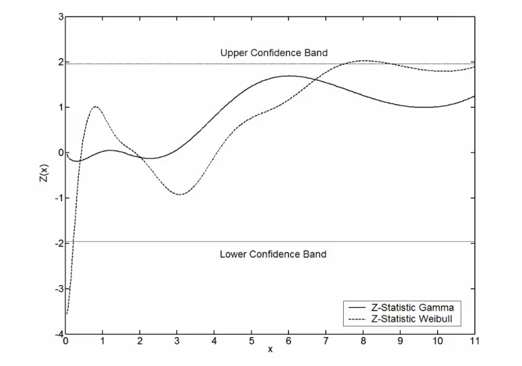
Figure 2 provides an example. 500 random values from a Gamma G(1.5,1) were drawn and the
density was estimated by the asymmetric HG estimator with a gamma and a Weibull start. Figure 2 shows that both estimators perform well. As expected, the correction factor for the gamma start estimator is close to one, whereas some nonparametric correction is done for the Weibull start estimator, especially in the tail of the density. Figure 3 plots the Z-statistic given in (4.17) for both estimators. Whereas the Z-statistic for the gamma start estimator is always within the confidence bands, the Weibull start estimator is outside at some of the points. The violation is not large. This is because the Weibull can capture the above gamma specification fairly well. Figure 4 shows the same procedure when the true density is LN(0,1). The correction factors for both estimators indicate that neither a
gamma nor a Weibull can capture the tail of lognormal data. Also the close fit shows that although the
parametric start is clearly wrong, the density is fitted quite well due to the nonparametric correction for misspecification.
The present framework can also be used to test if the data was generated by a particular parametric modelf(x, θ) where θ∈Θ (H0). We propose the global test statistic
Tn =nb1/2
Z ∞
0
ϕ(x) [ˆr(x)−1]2dx, (4.18)
where ϕ(x) is some appropriately chosen weighting function. Asymptotic normality of this statistic
could be shown using results given in Fernandes and Monteiro (2005). It is, however, well known that similar tests based on symmetric kernel estimators are very sensitive to the choice of the smoothing parameter. Fan (1995, 1998) reports that for a wide range of values of the smoothing parameter the test statistics can have large skewness and kurtosis exhibiting behaviour more like χ2 tests than normal
tests. Size distortions can therefore be quite large. Fan shows that the parametric bootstrap can solve these problems, and we therefore propose the following standard procedure to determine the critical value of the test:
Step 1. Draw a random sample of sizen,©X∗
j
ªn
j=1, from the distribution with density functionf
³ x,ˆθ´
whereˆθis estimated by maximum likelihood from the original data. This is the bootstrap sample. Hence conditional on the random sample {Xj}nj=1, the boostrap sample satisfies H0 with θ =θ0.
Step 2. Use the bootstrap sample©X∗
j
ªn
j=1 in place of the original data to compute Tn. Call it T
∗
n.
Step 3. Repeat Step 1 and Step 2 for a large number of times, say B, and obtain the empirical distribution function of©Tn,r∗
ªB
r=1, called the bootstrap distribution.
Let Cα be the upper α−percentile of the calculated bootstrap distribution. Then reject the null
hypothesis at significance level α if Tn > Cα. Tn is small under the null hypothesis for two reasons.
First because the parametric model is correct and rˆ(x) should be close to one. Second because the
estimator is unbiased and should, therefore, be more precisely measured under the null than under the alternative hypothesis. We therefore expect the power of this semiparametric test to be greater than that of pure nonparametric versions of this kind of specification tests.
Furthermore the statistic given in (4.18) can be used for an adequate choice of a parametric start. The density under consideration can be estimated with different parametric starts. Then one can choose that parametric start density for which the value of the above statistic is the smallest.
4.7
Extensions
Before turning to the Monte Carlo results, wefinally would like to mention that our approach can easily be extended to the estimation of densities which have support on the interval [0,1]. An application in credit risk is the estimation of the density of recovery rates at default, see Renault and Scaillet (2004), Hagmann, Renault and Scaillet (2005). To accommodate two known boundaries, Chen (1999) intro-duced asymmetric kernels based on the beta distribution KB with parameters(x/b+ 1,(1−x)/b+ 1) given by KB µ t;x b + 1, (1−x) b + 1 ¶ = t x/b(1 −t)(1−x)/bI(0≤t≤1) B(x/b+ 1,(1−x)/b+ 1) ,
where B(·) denotes the beta function. The support of the kernel again matches the support of the
density and the resulting estimates are free of boundary bias. An obvious parametric start is given
by the beta family of densities. Writing Equation (4.2) using a beta kernel and performing analogous
calculations as before, one can establish the bias and variance of the beta kernel version of the LMBC estimator.
K is the beta kernel is given for q≥2 by: Bias³f˜bB(x)´ = 1 2x(1−x)f0(x) £ r(2)(x)−r(2)(x, θ02)¤b+o(b), Var³f˜bB(x)´ = ( 1 2√πn− 1b−1/2 {x(1−x)}−1/2f(x) if x/b→ ∞, Γ(2κ+1) 21+2κΓ2(κ+1)n−1b−1f(x) if x/b →κ.
The variance of this semiparametric density estimator coincides with that of the pure nonparametric beta kernel estimator. We refer to Chen (1999). Compared to the bias of the nonparametric beta kernel estimator, first order derivative terms of the true density vanish (asq ≥2) in the bias expression of the semiparametric estimator. Also, f(2)(x) is replaced by f
0(x) £ r(2)(x) −r(2)(x, θ0 2) ¤
. The same remarks apply for the comparison of these biases as before.
Finally the LMBC approach could be extended to a multivariate setting through use of product kernels without any particular difficulties .
5
Monte Carlo study
In this section we evaluate the finite sample performance of most of the estimators considered in the
previous section. For estimators involving asymmetric kernels, we focus on the gamma kernel. This because, as demonstrated earlier on, the use of the gamma kernel allows us to obtain semiparametric estimators in closed form. This attractive property of the asymmetric gamma kernel does not transfer to the RIG kernel and the IG kernel, where numerical integration and optimization has to be used to obtain density estimates. This makes the RIG kernel and the IG kernel somewhat less attractive for a large scale simulation study as well as empirical work11. To the best of our knowledge, it is the first
time that various semiparametric density estimators are compared on a finite sample basis.
5.1
Semiparametric estimators and test densities
We run a Monte Carlo simulation for the following semiparametric density estimators:
• the pure nonparametric gamma kernel estimator (G1),
11We examined the performance of the RIG kernel and the IG kernel in case of the HG estimator, where a closed form solution is available. Results for the RIG were similar as for the HG estimator relying on the gamma kernel, whereas the IG version performed significantly worse. This is in line with results reported in Scaillet (2004), who examines the performance of those asymmetric kernels in a pure nonparametric setting.
• the uncorrected semiparametric HG estimator with a gamma start, using the Epanechnikov kernel
(SHGG),
• the local linear HG estimator with a gamma start given in Equation(2.6), using the Epanechnikov kernel (SHGGC),
• the semiparametric HG estimator with a gamma start given in Equation (4.8), using the gamma
kernel (AHGG),
• the LMBC estimator with a gamma start and a log linear correction factor, given in Equation
(4.12) (ALMBC),
• the local log linear estimator using the gamma kernel given in Equation(4.13) (ALLL).
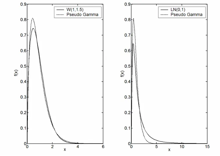
We compare these estimators on three different test densities: a Gamma G(1.5,1), a Weibull
W(1,1.5) and a lognormal LN(0,1). The G1 estimator takes the role of the benchmark for the other estimators. A useful semiparametric estimator should at least in some cases outperform its pure non-parametric competitor. The SHGG, SHGGC and AHGG are all HG type estimators which use the gamma as a start density. The only source of bias reduction achieved by these estimators is provided by the global parametric start. Note that the SHGGC is a direct competitor to AHGG. Indeed they are both free of boundary bias. We will see that the HG estimator with a symmetric kernel without any boundary correction (SHGG) yields in fact very unsatisfactory results. All the considered HG type density estimators should perform well for the gamma test density since the correction factor can be estimated without bias. We also expect them to perform well for the Weibull test density. This because the gamma start can come close to a Weibull density, implying that the correction factor exhibits only small curvature and is therefore simple to estimate. This is demonstrated in the left panel of Figure 512, where the Weibull and corresponding pseudo gamma density are plotted. The right panel shows the pseudo gamma when the true data is drawn from the lognormal test density. In this case, the gamma does not provide a reasonable start. The correction factor exhibits high curvature and is therefore more difficult to estimate. Also recall our example in Figure 4. The ALMBC estimator should perform better in this situation, since the additional local model for the correction factor theoretically leads to an improvement over the HG type estimators. Finally, the performance of the ALLL estimator is of interest because it does not need any global parametric start but provides a pure local bias correction13. 12The pseudo gamma parameter values are calculated via Monte Carlo integration based on a sample of one million Weibull or lognormal random values.
13For comparison purposes, we also tried to implement a local log linear estimator with a symmetric kernel. However, this estimator was not suitable for a large scale simulation study, since computation in the boundary of the density requires numerical search procedures in each single step.
5.2
Design of the Monte Carlo study
The performance measures we consider are the integrated squared error (ISE) and the weighted inte-grated squared error (WISE) of the various estimators:
ISE = Z +∞ −∞ n ˜ f(x)−f(x)o 2 dx, WISE = Z +∞ −∞ n ˜ f(x)−f(x)o2x2dx.
The WISE allows us to capture the tail performance of our estimators. The experiments are based on 1,000 random samples of length n= 100, n = 200, n = 500and n= 1,000. We provide a "best case" analysis, meaning that for each simulated sample the ISE was computed over a grid of bandwidths and the minimum value was chosen. The WISE is computed in each simulation step with the same
bandwidth as the ISE14. Numerical integration was performed by Gauss Legendre quadrature with 96
knots.
5.3
Numerical issues
In afirst simulation step the SHGGC estimator surprisingly performed much worse than the uncorrected estimator SHGG. The reason was that the correction factor can sometimes, especially in the boundary, become too influential. Following H&G, we implemented a trimmed version of the estimator given in Equation (2.6) using f³x,ˆθ1 ´ ˆ r(x) = 1 n n X i=1 Kh(Xi−x) min ⎛ ⎝ f ³ x,ˆθ1 ´ f³Xi,ˆθ1 ´, a ⎞ ⎠, f³x,ˆθ1 ´ ˆ g(x) = 1 n n X i=1 Kh(Xi−x)(Xi−x) min ⎛ ⎝ f ³ x,ˆθ1 ´ f³Xi,ˆθ1 ´, a ⎞ ⎠,
where a > 0. Similar "clipping" precautions in the density estimation setting are recommended by Abramson (1982) and Terrell and Scott (1992). This trimming procedure successfully solved the
nu-merical problems for the symmetric kernel based estimator. From our experience, a ∈ [10,50] is a
satisfactory choice. In fact within that range, the Monte Carlo results for this estimator were only insignificantly influenced. The semiparametric asymmetric kernel density estimators did not suffer from
14Another procedure would be to compute the WISE as well over a grid of bandwidths and choose the minimum value in each simulation step. We do not follow this because we want to evaluate the tail performance of our estimators given that they fit the whole density well. This is achieved by computing the WISE with the ISE-minimizing bandwidth in each simulation step.
the same numerical problem and were implemented without any trimming in the form described in Section 4.
5.4
Results
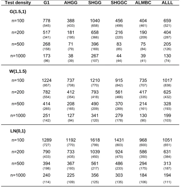
Table 1 shows the simulation results for the MISE criterion with standard errors of each simulation experiment reported in brackets. The AHGG estimator brings large improvements over the G1 estimator when the parametric start is true or close to the true density. Even for the lognormal example, its performance is still slightly better. This is because the uniform distribution, which is the implicit start for the G1 estimator, is quite a conservative start. The performance of the ALMBC is especially interesting when the parametric start is a poor specification for the true density. Whereas the ALMBC shows as expected a similar performance as the AHGG estimator for the gamma and Weibull test densities, the additional local model for the correction factor brings another 20% improvement for the lognormal test density. The ALMBC estimator also performs uniformly better than the ALLL estimator, which yields compared to the G1 estimator an improvement between 15-25% across all test densities and sample sizes. The ALLL however does not rely on a parametric start and may perform better when misspecification is stronger than the one considered here.
The poor performance of the SHGG estimator demonstrates how important the boundary bias feature is in the semiparametric framework considered in this paper. Even when the parametric start is correct, SHGG performs worse than the pure nonparametric G1 estimator. Partly, this is because the boundary bias prevents an enlarged bandwidth. Although the trimmed local linear version of this estimator brings a large improvement compared to the uncorrected symmetric estimator, its performance is considerably lower than that of the AHGG estimator. In the slightly misspecified Weibull case with a sample size of 1,000, the MISE of the AHGG estimator shrinks to 46% of the MISE of the SHGGC estimator. Chen (2000) has already reported that the asymmetric kernel estimator performs better than its symmetric local linear competitor. The outperformance in our case is however much larger, since the boundary bias problem magnifies in our semiparametric framework as mentioned earlier.
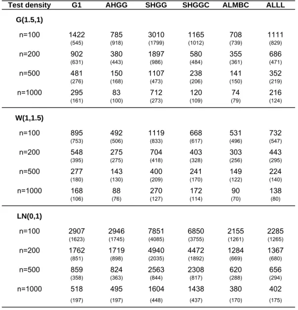
Table 2 shows the same information but for the WISE criterion and makes the power of the asymmet-ric estimators obvious. Those estimators perform much better in the tail of the density than estimators based on symmetric kernels. For the lognormal density which has the largest tail among the test den-sities, the WISE of the AHGG estimator is just one third of the WISE of its symmetric kernel based competitor SHGGC. We expect this relative advantage to increase for densities that have heavier tails than the lognormal density, e.g. Pareto distributions. This tail advantage of the asymmetric kernel is due to its changing shape as one moves away from the boundary. ALMBC exhibits excellent performance also with respect to the WISE criterion.
6
Empirical applications
In this section we illustrate the usefulness of our estimation approach with two empirical applications. The first one deals with health insurance data provided by a large Swiss health insurer. The second application deals with Brazilian income data.
6.1
Application to health insurance data
The Swiss health insurance system is heavily regulated by law. All residents in Switzerland have a compulsory base insurance which covers general health expenses. In the year 2002, approximately one third of total health expenses of 45 billion Swiss Francs were covered by this base insurance, which is offered by different private insurers.
Since the cost structure among different cantons in Switzerland is very different, we focus here on claims generated by residents of the canton of Zurich. The data considered is the net payment per client in the year 2002, covering claims for the base insurance only. We show how our approach can be used to compare the shape of the loss distribution for different subpopulations to better assess each underlying risk.
Table 3 shows the descriptive statistics of our dataset. It is evident that this dataset is highly skewed and exhibits large kurtosis. Also, the average payment varies significantly with the gender and age of the subpopulations. Obviously, the claim structure is also very different depending on whether the client lives in Zurich City or in rural area. We note that the "thought of solidarity" in the Swiss health system implies that clients with an age above 26 years pay all the same premium for their base insurance, independent of age and gender.
Figure 6 shows the loss distribution for the whole sample estimated for comparison purposes by the SHGGC estimator and our ALMBC estimator, both using a gamma start. These two estimators were the best symmetric and asymmetric estimators emerging from our Monte Carlo Study. To avoid numerical overflow, the original dataset was divided by 2,000. Then the resulting density has been back transformed. The bandwidth was calculated using the LSCV procedure described in Section 4.5. We report the bandwidth chosen for the transformed data for all considered estimators in Table 4. We also tried the ALLL estimator, but the resulting density cannot be distinguished by eye from that of the ALMBC estimator and is therefore not plotted. The shape of the loss distribution is very typical; we have a peak for the small claim sizes and then a very long tail. At first glance, the estimates for the symmetric and asymmetric estimator seem quite similar. The correction factor in the right panel of Figure 6 shows, however, that the asymmetric estimator produces a smooth tail, whereas the symmetric estimator features a bumpy behaviour. The picture shows that we have to correct around the mode and also in the tails. The correction factor further left to the picture (not shown) is increasing up to