3
Iranian Journal of Chemical Engineering Vol. 11, No. 2 (Spring 2014), IAChE
Dynamic Simulation and Control of Microbial
Cell Population in Continuous Bioreactors
A.R. Ehsani, A. Ghaemi∗
School of Chemical Engineering, Iran University of Science and Technology, Tehran, Iran
Abstract
Continuous bioreactors are critical unit operations in a wide variety of biotechnological processes. Due to the level of detail built in their mathematical formulation, cell population balance models represent the most accurate way of describing the microbial population heterogeneity in continuous bioreactor. In this work,the equation set of the model was solved numerically using rigorous'space–time conservation element and solution element' CE/SE method.MATLAB/Simulink pre-existing blocks are used for modeling and control of the different moments of cell mass distribution in a continuous bioreactor. For investigating the efficiency of automatic controller, 10% increase in maximum specific growth rate in Ks, was considered. The
set point for zeroth, first and second moments of distribution were taken to be; M0,sp=0.6706 , M1,sp=0.1541 , M2,sp=0.0505, which correspond to a dilution rate of
0.953 h-1 and 0.6 h-1. In the first case the controller response after 10 hours was
(0.92 h-1 ± .05), (0.87 h-1 ± 0.4) and (0.92 h-1 ± 0.2). For the second case the controller
response was close to set point(0.6 h-1 ± .001) after 20 hours.
Keywords: Continuous Bioreactor, Cell Population Balance, Dynamic Modeling,
CE/SE Method, Process Control
∗ Corresponding author: [email protected]
1. Introduction
The biochemical manufacturing industries are growing swiftly due to significant advancements in biotechnology and the high value of biochemical products. Typical biochemical processes involve batch, fed-batch and/or continuous bioreactors. In many bioprocess applications, continuous bioreactors are favored due to their advantages such as ease of operation and
higher productivity [1, 2].
4 Iranian Journal of Chemical Engineering, Vol. 11, No. 2 formation in microbial cultures, known as
cell population balance (CPB) models were first formulated by Fredrickson and his co-workers more than 40 years ago [4-7].
In spite of the advantages of CPB models, some significant difficulties can be found in their applications. First, the intrinsic physiological state functions which appear as parameters in such models are unknown for most cell systems and their determination requires information at the single-cell level. Second, CPB equations typically consist of first order partial integro-differential equations describing the dynamics of cell properties distribution, coupled in a nonlinear fashion with ordinary integro-differential equations accounting for substrate consumption and/or product formation. Thus, they are characterized by considerable mathematical complexity.
In population balance equations the intracellular state is characterized by a variable such as cell age or mass. Generally, the CPB problem cannot be solved analytically, although some interesting approaches exist for simplified versions of the problem [8-10]. In the last decades, most attempts were to solve numerical age and mass structured CPB models. Finite difference method was applied by Kurtz et al. to discretize an age-structured CPB model [11]. Orthogonal collocation on finite elements to discretize a simplified version of a yeast cell population model has been applied to develop a control strategy in order to reduce oscillations in yeast cultures [12]. The same numerical method has been applied for bifurcation analysis and model reduction of yeast population models [13-14]. Mantzaris et al. have presented several finite
differences, spectral and finite element algorithms to solve CPB models accurately and rapidly [15-18]. They also developed nonlinear feedback laws for controlling different moments of cell mass distribution in single stage and productivity in a multi-staged CPB model in a continuous bioreactor [19-20]. The mentioned algorithms all assume that the boundaries of the intracellular state space are fixed. Mantzaris
et al. showed that CPB models are able to
predict multiple solutions for steady state behavior [21]. These steady states can vary over several orders of magnitude. Hence, fixed boundary algorithms can produce inaccurate results for these kinds of problems. Thus, moving boundary algorithms are required to treat these challenges. Kavousanakis et al. proposed a free boundary algorithm for numerically solving CPB problems [22]. Recently, some researchers have considered source of heterogeneity in cell population [29] and also some works investigate combination of metabolic network and cell population to better describe cell behavior in community level [30-31].
Iranian Journal of Chemical Engineering, Vol. 11, No. 2 5 2. CPB modeling
Consider a population of cells growing in a continuous bioreactor. Each individual cell in the microbial population contains different quantities of r biochemical components (DNA, RNA, protein, etc.). Assume that
x=[x1, x2, …,xr] denote the physiological
state vector. The domain of physiological state space is defined asG=[x , xmin max]⊂R+r
where xmin, xmax denote the vectors containing the minimum and maximum values, respectively, for the amounts of the r
components of the cells. For simplicity and without loss of generality, it is assumed
xmin=0 and xmax=1. The state of the entire
population is described by a time-dependent function N(x,t)where N(x,t)dx represents the number of cells per unit biovolume that at time t have intracellular content between x
and x+dx. The total number of cells per unit biovolume (cell density) and the concentration of the i-th biomass component are respectively obtained from the zeroth and first moments of the state distribution function:
max
min
( , ) x ( , )
t x
N x t =
∫
N x t dx (1)max
min
, ( ) ( , ) , 1,...,
x
b i x i
N t =
∫
x N x t dx i= r (2)The sum from 1 to r of all expressions (integrations are performed over the entire r -dimensional space of G) defined in equation 1 yields the total biomass concentration at time t.
The number density function n(x,t)is defined as the state distribution function divided by the total number of cells per unit biovolume at time t:
( , ) ( , )
( , )
G
N x t n x t
N x t dx
=
∫
(3)Let S=[S1, S2,…,Ss]denote the substrate
concentration vector (assuming s substrate). A cell population balance model includes information about nutrient uptake, growth, division and birth at the single-cell level. The nutrient consumption process is characterized by the s-dimensional consumption rate vector
q (x,S) = [q1 (x,S), q2 (x,S),…,qs (x,S)] where
qi (x,S), i=1,…,s denotes the single-cell rate
of consumption of the i-th substrate. The growth process is represented by the r-dimensional single-cell growth rate vector
r(x,S)=[r1(x,S), r2(x,S),…,rr(x,S)] where
ri(x,S), i=1,…,s denotes the rate of increase
in the amount of the i-th cellular constituent. The cell division is described by the division
rateΓ(x,S). The birth process is described by
the partition probability density function partition p(x,y,S).This function expresses the probability that a mother cell with physiological state vector y gives birth to a daughter cell with physiological state vector
x. This function must satisfy the
normalization condition:
max min
( , , ) 1
x
x p x y S dx=
∫
(4)6 Iranian Journal of Chemical Engineering, Vol. 11, No. 2 ( , , ) 0, i i , 1,...,
p x y S = ∀ >x y i= r (5)
Finally, the probability of a dividing cell with physiological state vector y to produce a daughter cell of state x must be equal to the probability of producing a daughter cell of state y - x, i.e.
( , , ) ( , , )
p x y S = p y x y S− (6)
Under assumptions and the process description above, the dynamics of the distributionN(x,t), is given by the following cell population balance model:
max
( , )
[ ( ) ( , )] ( ) ( , )
( , ) 2 ( , ) ( , ) ( , )
∂ ∂
+ + Γ
∂ ∂
+ =
∫
x Γx
N x t
R x N x t x N x t
t x
DN x t y S P x y N y t dy
(7)
The first term quantified is accumulation; the second denotes the loss of cells with content
x due to intracellular reactions. The third term represents division to yield cells with lower content; the fourth term is the dilution term describing the rate by which cells exit the reactor. The last term (on the right hand side) describes the birth of cells of content x from the division of all cells with greater intracellular content. Moreover, each division leads to the birth of two daughter cells, thus a factor of 2 multiplying the integral term. The initial and boundary conditions for N(x,t) are denoted as follows:
0
( ,0) ( )
N x =N x (8)
(0, ) (0, ) (1, ) (1, )
R S N t =R S N t (9)
In addition, Kurtz et al. used the following boundary condition for cell distribution:
max min
(0, ) 2 x ( , ) ( , )
x
N t =
∫
Γ x S N x t dx (10)The boundary condition simply states that the number of cells at mass zero, N(x,t), must be twice the number of divided cells. The CPB equation is coupled with the equation of substrate consumption. The substrate balance is written as:
max min
( f ) x ( , ) ( , )
x
dS
D S S q x S N x t dx
dt = − −
∫
(11)The initial condition for S is expressed as:
0
(0)
S =S (12)
3. Mathematical formulation of mass-structured CPB
A common simplification to the general structured cell population balance model presented above concerns the case of a single physiological state x. In this work, physiological state vector consisting of cell mass m was considered. This is quite meaningful in bioreactors where cell growth and division are strongly dependent on cell mass. In this case, the cell population model takes the form (m∈[0,1]):
1
( , )
[ ( , ) ( , )] ( ) ( , )
( , ) 2 ( , ) ( , ) ( , )
∂ + ∂ + Γ
∂ ∂
′ ′ ′ ′
+ =
∫
Γm
N m t
R m S N m t m N m t
t m
DN m t m S P m y N m t dm
Iranian Journal of Chemical Engineering, Vol. 11, No. 2 7 2
0 0
( ) /(2 ) 0
1 ( ,0)
2
m
N x e μ σ
σ π
− −
= (14)
The single cell growth rate is modeled as:
max
( , )
s
S R m S
K S
μ
= +
(15)
Where μmax and Ks are constants. The growth rate function models the tendency of cells to reach a maximum growth rate (μmax) at large substrate concentrations. The division rate function is modeled as:
0
( )
( , ) ( , )
1 m ( )
f m
m t R m S
f m dm
Γ =
′ ′
−
∫
(16)
Where f(m)is the division probability density function and it is taken to be a Gaussian distribution with the mean of μf and
standard deviation ofσf. The partition of the mother cells into two daughter cells is described by the partitioning function. It is assumed thatp m m( , ′)is a symmetric beta distribution, with a parameter of q, defined by the following equation:
1 1
1 1
( , ) 1
( , )
q q
m m
P m m
B q q m m m
− −
⎛ ⎞ ⎛ ⎞
′ = ⎜ ⎟ ⎜ − ⎟
′⎝ ′⎠ ⎝ ′⎠
(17)
The single-cell rate of consumption of substrate is modeled as:
1
( , )
R m S Y
(18)
Where, Y is a constant yield coefficient. Finally, it is assumed that no cell death occurs and that cells grow in one stage.
4. Numerical solution
As mentioned in previous sections, the CPB model is comprised of a coupled set of nonlinear algebraic, ordinary differential and integro-partial differential equations. Analytical solution is possible only under very limiting assumptions [23, 24]. Therefore, numerical solution is required when the population balance equation (PBE) model is utilized in open-loop and closed-loop simulations. In this work, theCE/SE method is used for solving the CPB model in continuous bioreactor.
The CE/SE method was developed by Chang and coworkers [25, 27] to calculate the numerical solution of partial differential equations. This method was originally developed to treat conservation laws in fluid dynamics but can be modified to solve the population balance equations [26]. This method is derived from first principles by enforcing local (and global) numerical flux conservation. It is well suited to the solution of partial differential equations where numerical diffusion is a concern (e.g. CBP model).
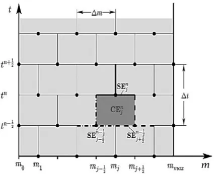
The application of CE/SE method requires the discrete treatment of both the mass as a physiological state and time coordinates. Fig. 1 shows the discretization of time (t) versus mass domain (m).
For demonstrating the strategy of the CE/SE method, the partial derivatives of the PBE will be considered in the form of a conservation law:
( )
,(
,) ( )
,0
N m t R m S N m t
t m
∂ ∂
+ =
∂ ∂
8 Iranian Journal of Chemical Engineering, Vol. 11, No. 2
Figure 1. Subdivision of the domain time t versus
mass m into conservation elements (CE) and solution elements (SE).
For derivation of this numerical method, integral form of this conservation law is taken into consideration:
( )
,(
,) ( )
,0
V
N m t R m S N m t
dV
t m
⎛∂ ∂ ⎞
+ =
⎜ ∂ ∂ ⎟
⎝ ⎠
∫
(20)
In this equation V denotes an arbitrary area element of the domain depicted in Fig. 1. Applying the Gauss divergence theorem to Eq. (20) results in:
(21)
Where S(V) is the boundary of the region V
and hr=(RN N, ) and d sr=d nσ r are vectors with dσ and nr denoting the area and the outward unit normal of a surface element on
S(V), respectively.
On the solution elements the state distribution function N, the flux term RN and the vector hr will be approximated by the first-order Taylor expansions N*, (RN)* and
∗
r
h around the center points (j,n) of each solution element n
j
SE , see Fig. 1. The state distribution function N, for example, is then approximated by:
(
)
( )
(
)
( ) (
)
* , ; , n n n
j m j j t j n
N m t j n =N + N m m− + N t t−
(22)
with n
j
N , ( )n
m j
N and ( )n
t j
N being the
values of N, ∂N/∂m and ∂N/∂t at (mj,tn),
respectively. As a consequence of the fact that N* has to satisfy the differential form (19) of the considered conservation law it follows that ( )n
t j
N can be substituted by:
( )
( )
n n
t j
j
RN N
m
⎛∂ ⎞
= −⎜ ∂ ⎟
⎝ ⎠ (23)
Demanding the integral form (20) of the conservation law to also be valid for the Taylor expansions within each conservation element n
j
CE leads to:
(24)
Where ( n)
j
S CE is the surrounding line
around n
j
CE which consists, as depicted in Fig. 1, of sections belonging to the three
neighboring solution elements 1/ 2
1/ 2
, −
−
n n
j j
SE SE
and 1/ 2
1/ 2
− +
n j
SE .
The line integral in Eq. (24) can be evaluated using a primeval function ψ for the
Iranian Journal of Chemical Engineering, Vol. 11, No. 2 9
( )
* *Ψ Ψ
RN and N
t m
∂ = ∂ =
∂ ∂ (25)
which have to be valid for such a primitive function, Chang [25] gives the following expression for the desired primitive function:
(
) (
)
(
)
(
)
(
)
(
)
(
)
(
)
(
)
(
)
(
)
2 2 Ψ , 1 1 2 2 = − − − ⎛∂ ⎞ + ⎜ ⎟ − − − ∂ ⎝ ⎠ ⎛∂ ⎞ +⎜ ⎟ − − ∂ ⎝ ⎠ nn n n
j j j j
n
n n
m j j
j n
n j
j
m t RN t t N m m
RN
t t N m m
t
RN
m m t t
m
(26)
Using the antiderivative ψ(m,t;j,n) the line integral in Eq. (24) can be evaluated by integrating around the conservation element
n j
CE as:
1 1 1 1
2 2 2 2
1 1 1 1
2 2 2 2
1 1 1 1
2 2 2 2
1 1 1 1
2 2 2 2
Δ Δ Ψ , Ψ , 2 2 Δ Δ Ψ , Ψ , 2 2 Δ Δ
Ψ , Ψ , 0
2 2 − − − − − − − − − − − − + + + + ⎛ − ⎞− ⎛ + ⎞ ⎜ ⎟ ⎜ ⎟ ⎝ ⎠ ⎝ ⎠ ⎛ ⎞ ⎛ ⎞ + ⎜ + ⎟− ⎜ + ⎟ ⎝ ⎠ ⎝ ⎠ ⎛ ⎞ ⎛ ⎞ + ⎜ + ⎟− ⎜ − ⎟= ⎝ ⎠ ⎝ ⎠
n n n n
j j j j
n n n n
j j j j
n n n n
j j j j
m m
m t m t
m t
m t m t
t m
m t m t
(27)
Substitution of Eq. (26) into Eq. (27) yields:
1/2 1/2 1/2 1/2
1/2 1/2 1/2 1/2
1/ 2
n n n n n
j j j j j
N N − N − s − s −
− + − +
⎡ ⎤
= ⎣ + + − ⎦
(28) With the abbreviation:
( )
( ) ( )
Δ 2( )
Δ Δ
4 Δ 4Δ
n
n n
n
j m j j
j
t RN
m t
s N RN
m m t
⎛∂ ⎞
= + + ⎜ ⎟
∂
⎝ ⎠
(29)
Eq. (28) in conjuncture with Eq. (29)
represents an explicit time marching scheme to compute the numerical solution of N at time tn from the previously calculated values
attn-1/2. The so far undefined numerical
analogue Nm to the partial derivative ∂N=∂m
can be determined according to[25], by:
( )
n n(
2 1)(
)
nm j j m j
N =W + ε− dN (30)
With:
(
)
(
( )
1( )
1)
(
1 1)
1 1
1 1
1 1
2 Δ
n n n n n
m j m j m j j j
dN N N N N
m − − − − + − + − = − − − (31)
The symbol n
j
W in Eq. (30) represents a weighted average of the numerical analogues of the partial derivative ∂N=∂m attn and mj, evaluated from the left and from the right-handside, respectively. The adjustable parameter ε controls the magnitude of the introduced numerical diffusion and has to be chosen between 0 and 1 [25].
In order to include the integral terms in the PBE into the CE/SE framework, an analytical integration of the Taylor expansion Eq. (22) of each solution element can be used. The sum over the contributions of all solution elements in one row gives a better approximation to the desired integrals in the model equations than in case of the finite volume methods, since the CE/SE method calculates the solution of N in addition to numerical analogues for the partial derivative
10 Iranian Journal of Chemical Engineering, Vol. 11, No. 2
Table 1. Parameter values used in the simulation.
Variable Value Variable Value
0
σ 0.05 Ks 0.2g l−1
0
μ 0.25 S0 2g l−1
f
σ 0.575 Sf 10g l−1
f
μ 0.125 q 40
max
μ 1 h−1 Y 0.5g g−1
For better visualization of the system behavior, the predicted dynamics of the state distribution function was presented in a three dimensional plot (Fig. 2). Different boundary conditions (Eqs. 9 & 10) are used for this
open loop simulation. Results were obtained
for D = 0.1 h-1 condition.Using Eq. 9 as
boundary condition the model cannot predict oscillations in state distribution function
N(m,t).As shown in Fig. 3b, N(m,t) displays
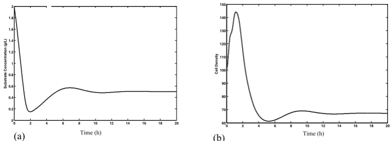
oscillatory behavior early on that subsides into the unchanging distribution. This behavior appears consistent with results presented elsewhere in the literature [18]. The open loop responses of total number of cells per unit biovolume (cell density) (Eq. 1) and substrate concentration are shown in Fig. 3. Simulation results were obtained for D = 0.1h-1.
Figure 2. Dynamic simulation of state distribution function, Numerical results for dt = 0.01
and dm= 0.01., (a) Eq. 9, (b) Eq. 10 as boundary condition.
0 2 4 6 8 10 12 14 16 18 20
0 0.2 0.4 0.6 0.8 1 1.2 1.4 1.6 1.8 2
Time (hr)
S
u
b
st
rat
e C
o
n
cen
tr
at
io
n
(g
/L
)
3a ) 0 2 4 6 8 10 12 14 16 18 20
60 70 80 90 100 110 120 130 140 150
Time (hr)
C
ell D
en
sit
y
3b )
Figure 3. Open loop simulation, Numerical results for dt = 0.01 and dm = 0.01,using Eq. 9 as boundary condition,
(a) substrate concentration, (b) cell density.
Time (h) Time (h)
(a) (b)
Iranian Journal of Chemical Engineering, Vol. 11, No. 2 11 Fig. 4 provides important information about
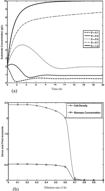
the results of CPB equation coupled with substrate concentration in continuous bioreactor. Dynamic behavior of cell population balance and the impact of different dilution rates on the steady state characteristics of the distribution as well as on the steady state substrate concentration are shown in Fig. 5. The steady state value for each case obtained from simulations results in t=13 h. Notice that as D increases, S increases first, smoothly. In the cases in which dilution rates are 0.1, 0.3 and 0.5 (h-1) steady state substrate concentration values are 0.5013, 0.8832 and 1.9273 (gl-1), respectively. For dilution rates greater than 0.5 (h-1) steady state substrate concentration increases more rapidly as D tends toμmax.When dilution rate value is equal toμmax, S closely approaches Sf (Fig. 4a). Obviously, the increase in cell density is accompanied by a decrease in the substrate concentration and vice versa. Therefore, the total number of cells per unit biovolume (cell density) and total biomass concentration at steady state (t = 13h), zeroth and first moments of the state distribution function, respectively, decrease in a manner similarly explained about substrate concentration (Fig. 4b). As the dilution rate approaches the value of the maximum specific growth rate (μmax), the system reaches washout conditions. In this simulation Eq. 10 is used as boundary condition. Also, the use of Eq. 9 produces qualitatively similar results.
5. Automatic control of the process
Controlling the influence of manipulations in the operating and molecular parameters on
the different moments of the cell mass distribution in a continuous bioreactor is an important control objective in many bioprocess engineering applications. In some bioprocesses, certain metabolites of interest are only being produced during the last part of the cell cycle where cell mass is bigger. Therefore, for increasing the production of the metabolite, it is necessary to achieve a maximum possible in the zeroth and first moments of cell mass distribution and the minimum possible in second moment.
0 2 4 6 8 10 12 14 16 18 20 0
1 2 3 4 5 6 7 8 9 10
Time (hr)
S
u
b
st
ra
te C
o
n
cen
tr
at
io
n
(g
/L
)
D = 0.1 D = 0.3 D = 0.5 D = 0.7 D = 1.0
4a )
0 0.1 0.2 0.3 0.4 0.5 0.6 0.7 0.8 0.9 1 0
0.5 1 1.5 2 2.5
Dilution rate (1/hr)
Ze
ro
s a
nd Fi
rs
t m
o
m
ent
s
Cell Density Biomass Concentration
4b )
Figure 4. Open loop simulation. (a) Substrate
concentration, (b) Steady state cell density (o) and biomass concentration (), as a function of the dilution rate.
Time (h)
Dilution rate (1/h)
(a)
12 Iranian Journal of Chemical Engineering, Vol. 11, No. 2 Using MATLAB/Simulink environment and
its pre-existing packages facilitates simulating automatic control procedures for a wide variety of processes. Recently, Ward et al. developed a new Simulink block for automatic control of continuous crystallization process [28].
In the present work, a similar framework was used for designing an automatic controller for investigating the impact of dilution rate manipulations and other disturbances on the cell density (zeroth moment), biomass concentration (first moment) and second moment as different controlled outputs. As it is depicted in section 2, these moments are respectively defined in the following equations:
1
0( ) 0 ( , )
M t =
∫
N m t dm1
1( ) 0 ( , )
M t =
∫
mN m t dm1 2
2( ) 0 ( , )
M t =
∫
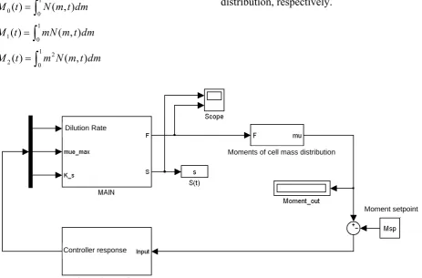
m N m t dmFig. 5 shows the Simulink block diagram developed for controlling zeroth, first and second moments of the cell mass distribution in a continuous bioreactor. The model contains several blocks which specify all of the model properties, conventional arithmetic operations, inputs and outputs. For better visualization, some blocks are summarized in subsystems which introduce the part of simulation that is accomplished inside the subsystem. The main subsystem contains m-files and blocks for solving the couple of cell population and substrate balance equations. The Simulink block diagram includes two other important subsystems, moment calculator and automatic controller that contain m-file and blocks for calculation and controlling different moments of cell mass distribution, respectively.
Figure 5. Simulink block diagram for a closed loop simulation and control of cell population balance model. Dilution Rate
Moments of cell mass distribution
Controller response
Iranian Journal of Chemical Engineering, Vol. 11, No. 2 13 The results of closed loop simulations are
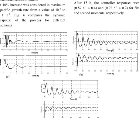
presented in Figs. 6 and 7, which show the temporal change of zeroth, first and second moments as controlled outputs. In this case, the automatic control of the process was simulated using conventional PID feedback control methodology. In all cases, the manipulated variable was dilution rate. In addition to changes in the set point, in all cases a step change in the maximum specific growth rate and saturation constant of the
Michaelis-Menten kinetics (Ks) were
considered as disturbances.
A 10% increase was considered in maximum specific growth rate from a value of 1h-1 to 1.1 h-1. Fig. 6 compares the dynamic response of the process for different moments
of cell mass distribution. The initial dilution rate in all simulations was taken to be equal to 0.1 h-1. The set point for zeroth, first and second moments of distribution was taken to be; a) M0,sp =0.6706, b) M1,sp =0.1541, c)
2,sp 0.0505
M = , which correspond to a
dilution rate of 0.953 h-1. For zeroth moment, the controlled output exhibited a good consistency with set point after 10 h and approached expected dilution rate (0.92 h-1 ±
.05). For first and second moments, the controlled outputs exhibited undershoot. After 15 h, the controller responses were (0.87 h-1 ± 0.4) and (0.92 h-1 ± 0.2) for first and second moments, respectively.
0 5 10 15 20 25 30 35 40 45 50
-0.5 0 0.5 1 1.5 2 2.5
Time (hr)
D
ilution
ra
te
0 5 10 15 20 25 30 35 40 45 50
0 0.5 1 1.5 2
Time (hr)
0t
h
m
o
m
ent
6a )
0 20 40 60 80 100 120 140 160 180 200
-0.5 0 0.5 1 1.5
Time (hr)
D
ilu
tio
n
r
a
te
0 20 40 60 80 100 120 140 160 180 200
0 0.1 0.2 0.3 0.4 0.5
Time (hr)
Fi
r
st
m
o
me
nt
6b )
0 50 100 150 200 250 300
-0.5 0 0.5 1 1.5 2
Di
lu
ti
o
n
r
a
te
Time (hr)
0 50 100 150 200 250 300
0 0.05 0.1 0.15 0.2
Time (hr)
S
econ
d
m
o
m
e
n
t
6c )
Figure 6. Closed loop simulation. Dynamic response of continuous bioreactor to a 10% increase in μmax. Setpoints
are (a) M0,sp=0.6706, (b) M1,sp =0.1541, (c) M2,sp=0.0505 corresponding to D = 0.1 h-1.
Time (h)
Time (h)
Time (h) Time (h)
Time (h)
Time (h)
(a) (b)
14 Iranian Journal of Chemical Engineering, Vol. 11, No. 2 6. Conclusions
The dynamic model of cell population in continuous bioreactor is used for describing characteristics of state distribution function. The model is solved numerically using the CE/SE method. The ability of the automatic controllers to achieve the desired objectives was evaluated through closed loop simulations. Set points for the different moments of cell mass distribution were determined from a solution for the steady state population balance model. The outputs are driven to their set points by a feedback controller which manipulates dilution rate. Three different moments of the cell mass distribution are controlled as outputs: (a) the cell density, (b) the biomass concentration, and (c) the second moment of the distribution. The controller achieved the desired closed-loop response in all cases. The accurate responses in closed loop simulations showed the potential of pre-existing MATLAB/Simulink packages for system identification and control. It can also facilitate rapid model development for a wide variety of chemical and biochemical processes.
References
[1] Lee, J.M., Biochemical Engineering, Prentice-Hall, Englewood Cliffs, p. 150, (1992).
[2] Shuler, M.L. and Kargi, F., Bioprocess engineering: Basic concepts, Prentice Hall, Englewood Cliffs, p. 20, (1992). [3] Daoutidis, P. and Henson, M.A.,
"Dynamics and control of cell populations in continuous bio-reactors", AIChE Symposium Series, 274, (2002). [4] Henson, M.A., "Dynamic modeling and
control of yeast cell populations in continuous biochemical reactors", Comput. Chem. Eng., 27, 1185, (2003). [5] Fredrickson, A.G., Ramkrishna, D. and
Tsuchiya, H.M., "Statistics and dynamics of prokaryotic cell populations", Math. Biosci., 1, 327, (1967).
[6] Eakman, J.M., Fredrickson, A.G. and Tsuchiya, H.M., "Statistics and dynamics of microbial cell populations", Chem. Eng. Prog., 62, 37 (1966).
[7] Tsuchiya, H.M., Fredrickson, A.G. and Aris, R., "Dynamics of microbial cell populations", Adv. Chem. Eng., 6, 125, (1966).
[8] Liou, J.J., Sriene, F. and Fredrickson, A.G., "Solutions of population balance models based on a successive generations approach", Chem. Eng. Sci., 52, 1529, (1997).
[9] Trucco, E., "Mathematical models for cellular systems, The von Foerster equation. Part 1", Bull. Math. Biophys., 27, 285, (1965).
[10] Trucco, E., "Mathematical models for cellular systems, The von Foerster equation. Part 2", Bull. Math. Biophys., 27, 449, (1965).
[11] Kurtz, M.J., Zhu, G.Y., Zamamiri, A., Henson, M. and Hjortso, M.A., "Control of oscillating microbial cultures described by population balance models", Ind. Eng. Chem. Res., 37, 4059, (1998).
Iranian Journal of Chemical Engineering, Vol. 11, No. 2 15 [13] Zhang, Y., Zamamiri, A.M., Henson,
M.A. and Hjortso, M.A., "Cell population models for bifurcation analysis and nonlinear control of continuous yeast bioreactors", J. Process Control, 12, 721, (2002).
[14] Zhang, Y., Henson, M.A. and
Kevrekidis, Y.G., "Nonlinear model reduction for dynamic analysis of cell population models", Chem. Eng. Sci., 58, 429, (2003).
[15] Mantzaris, N.V., Daoutidis, P. and Srienc, F., "Numerical solution of multivariable cell population balance models, I: Finite differences method", Comput. Chem. Eng., 25, 1411, (2001). [16] Mantzaris, N.V., Daoutidis, P. and
Srienc, F., "Numerical solution of multivariable cell population balance models, II: Spectral method", Comput. Chem. Eng., 25, 1441, (2001).
[17] Mantzaris, N.V., Daoutidis, P. and Srienc, F., "Numerical solution of multivariable cell population balance models, III: Finite Element method", Comput. Chem. Eng., 25, 1463, (2001). [18] Mantzaris, N.V., Liou, J.J., Daoutidis,
P. and Srienc, F., "Numerical solution of a mass structured cell population balance model in an environment of changing substrate concentration", J. biotechnol.,71,157, (1999).
[19] Mantzaris, N.V. and Daoutidis, P.,"Cell population balance modeling and control in continuous bioreactors", J. Process Control, 14, 775, (2004).
[20] Mantzaris, N.V., Srienc, F. and Daoutidis, P., "Nonlinear productivity control using a multi-staged cell population balance model", Chem. Eng. Sci., 57, 1, (2002).
[21] Mantzaris, N.V., "Stochastic and deterministic simulations of heterogeneous cell population dynamics", J. Theoret. Biology, 241, 690, (2006).
[22] Kavousanakis, M.E., Mantzaris, N.V. and Boudouvis, A.G., "A novel free boundary algorithm for the solution of cell population balance models", Chem. Eng. Sci., 64, 4247, (2009).
[23] Hjortso, M.A. and Nielsen, J.,
"Population balance models of autonomous microbial oscillations", J. biotechnol., 42, 255, (1995).
[24] Hjortso, M.A. and Nielsen, J., "A conceptual model of autonomous oscillations in microbial cultures", Chem. Eng. Sci., 49, 1083 , (1994). [25] Chang, S.C., "The method of
space-time conservation element and solution element: A new approach for solving the Navier–Stokes and Euler equations", J. Comput. Phys., 119, 295, (1995).
[26] Motz, S., Mitrovi, A. and Gilles, E.D., "Comparison of numerical methods for the simulation of dispersed phase systems", Chem. Eng. Sci., 57, 4329, (2002).
[27] Young, L., Chang, S.C. and Jorgensen, S.B., "A novel partial differential algebraic equation (PDAE) solver: Iterative space–time conservation element/solution element (CE/SE) method", Comput. Chem. Eng., 28, 1309, (2003).
[28] Ward, J.D. and Yu, C.C., "Population balance modeling in Simulink: PCSS", Comput. Chem. Eng., 32, 2233, (2008). [29] Stamatakis, M., "Cell population
16 Iranian Journal of Chemical Engineering, Vol. 11, No. 2 modeling frameworks: Conditional
equivalence and hybrid approaches", Chem. Eng. Sci., 65, 1008, (2010).
[30] Pigou, M. and Morchain, J.,
"Investigating the interactions between physical and biological heterogeneities in bioreactors using compartment, population balance and metabolic models", Chem. Eng. Sci., 126, 267, (2015).