Int. J. Industrial Mathematics Vol. 1, No. 1 (2009) 19-39
Numerical solution of fuzzy initial value problems
under generalized dierentiability by HPM
M. Ghanbari
Department of Mathematics, Mazandaran University, Babolsar, Iran.
|||||||||||||||||||||||||||||||-Abstract
In this work, the Homotopy Perturbation Method (HPM) is implemented for nding ap-proximate solution of the Fuzzy Initial Value Problem (FIVP) involving generalized dif-ferentiability. This method is based upon homotopy perturbation theory. The comparison of the exact solution with approximate solution obtained by HPM is in detail. The results reveal that the method is very eective and simple.
Keywords : Fuzzy numbers; Fuzzy dierential equations; Generalized dierentiability; Homotopy perturbation method.
||||||||||||||||||||||||||||||||{
1
Introduction
The concept of the fuzzy derivative was rst introduced by Chang and Zadeh [10]. Later, Dubois and Prade [11] presented a concept of the fuzzy derivative based on the extension principle. Other methods have been discussed by Puri and Ralescu [26], Goetschel and Voxman [14], Seikkala [27] and Friedman et al. [12, 21]. Recently, Bede introduced a strongly generalized dierentiability of fuzzy functions in [6, 7] and studied in [8]. The Fuzzy Dierential Equation (FDE) and the FIVP were rigorously treated by Kaleva [22, 23], Seikkala [27], He and Yi [15], Kloeden [24] and Menda [25]. The numerical methods for solving FDEs are introduced in [1, 2, 3, 4]. In this paper, the FIVP under generalized dierentiability is solved via Homotopy Perturbation Method (HPM). First we replace the FIVP by its parametric form and then solve the new system which consist of two classic ordinary dierential equations with initial conditions, then check to see if this solution dene a fuzzy function. HPM introduced by He [17, 18, 19, 20] has been used by many mathematicians and engineers to solve various functional equations. In this method the solution is considered as the sum of an innite series which converges rapidly to the accurate solutions. Using homotopy technique in topology, a homotopy is constructed with
an embedding parameter p 2 [0; 1] which is considered as a small parameter. The structure of this paper is organized as follows. In Section 2, some basic denitions which will be used later in the paper are provided. In Section 3, we present the dierent parametric forms of the FIVP by using the strongly generalized dierentiability concept. In Section 4, we state the basic concepts of HPM, and apply this method on parametric forms obtained in the previous section. In Section 5, we use the HPM for solve two FIVPs. We conclude in Section 6.
2 Preliminaries
Denition 2.1. A fuzzy number is a function u : < ! [0; 1] satisfying the following properties:
(i) u is normal, i.e. 9x02 < with u(x0) = 1,
(ii) u is a convex fuzzy set,
(iii) u is upper semi-continuous on <,
(iv) fx 2 < : u(x) > 0g is compact, where A denotes the closure of A.
The set of all these fuzzy numbers is denoted by E. Obviously, < E. Here < E is
understood as < = ffxg: x is usual real numberg. For 0 < r 1, denote [u]r= fx 2 < :
u(x) rg and [u]0 = fx 2 < : u(x) > 0g. Then it is well-known that for each r 2 [0; 1],
[u]r is a bounded closed interval. For u; v 2 E, and 2 <, the sum u v and the product
u are dened by
[u v]r = [u]r+ [v]r= fx + y : x 2 [u]r; y 2 [v]rg; 8r 2 [0; 1];
[ u]r= [u]r = fx : x 2 [u]rg; 8r 2 [0; 1]:
Dene D : E E ! <+Sf0g by the equation
D(u; v) = sup
0r1fmax[ jur vrj; jur vrj ]g; (2.1)
where [u]r = [ur; ur]; [v]r = [vr; vr]. Then it is easy to show that D is a metric in E.
Using the results in [13], we know that
(i) D(u w; v w) = D(u; v); 8u; v; w 2 E,
(ii) D( u; v) = jjD(u; v); 8 2 <; u; v 2 E, (iii) D(u v; w e) D(u; w) + D(v; e); 8u; v; w; e 2 E, (iv) (E; D) is a complete metric space.
Theorem 2.1. [28] If we dene j : E ! C[0; 1] C[0; 1] by j(u) = (u; u), where
u; u : [0; 1] ! <; u(r) = ur; u(r) = ur, then j(E) is a closed convex cone with vertex
(i) j(s u t v) = s j(u) t j(v); 8u; v 2 E; s; t 0; (ii) D(u; v) =k j(u) j(v) k :
Therefore, another denition for a fuzzy number which yields the same E is as follows [22]:
Denition 2.2. An arbitrary fuzzy number in the parametric form is represented by an ordered pair of functions (u(r); u(r)), 0 r 1; which satisfy the following requirements. (i) u(r) is a bounded left continuous nondecreasing function over [0; 1].
(ii) u(r) is a bounded left continuous nonincreasing function over [0; 1]. (iii) u(r) u(r); 0 r 1:
A crisp number is simply represented by u(r) = u(r) = ; 0 r 1.
We recall that for arbitrary fuzzy numbers u = (u(r); u(r)), v = (v(r); v(r)) and real number k,
(a) u = v if and only if u(r) = v(r) and u(r) = v(r).
(b) u v = (u v; u v) = (u(r) + v(r); u(r) + v(r)).
(c)
k u = 8 < :
(k u; k u) = (k u(r); k u(r)); k 0,
(k u; k u) = (k u(r); k u(r)); k < 0.
Note that ( 1) u may not be a fuzzy number when u be a fuzzy number. Similarly of (1), we dene
D(u; v) = sup
0r1fmax[ ju(r) v(r)j; ju(r) v(r)j ]g: (2.2)
In this paper, we represent an arbitrary fuzzy number by a pair of functions (u(r); u(r)); 0 r 1:
Theorem 2.2. [5]
(i) If we dene e0 = f0g, then e0 2 E is a neutral element with respect to addition, i.e.
u e0 = e0 u = u, for all u 2 E.
(ii) With respect to e0, none of u 2 E n <, has inverse in E (with respect to ).
(iii) For any a; b 2 < with a; b 0 or a; b 0 and any u 2 E, we have (a + b) u = a u b u, For general a; b 2 <, the above property does not hold.
(iv) For any 2 < and any u; v 2 E, we have (u v) = u v. (v) For any ; 2 < and any u 2 E, we have ( u) = (:) u.
Denition 2.4. Consider u; v 2 E. If there exists w 2 E such that u = v w, then w is called the Hukuhara dierence of u and v and it is denoted by u v.
In this paper the " " sign stands always for Hukuhara dierence and note that u v 6= u ( 1) v.
Denition 2.5. [6] Let f : (a; b) ! E and x0 2 (a; b). We say that f is strongly
generalized dierentiable on x0 (Bede dierentiable), if there exists an element f0(x0) 2 E,
such that
(i) for all h > 0 suciently small, 9f(x0+ h) f(x0); f(x0) f(x0 h) and the limits
(in the metric D)
lim h&0
f(x0+ h) f(x0)
h = limh&0
f(x0) f(x0 h)
h = f0(x0);
or
(ii) for all h > 0 suciently small, 9f(x0) f(x0+h); f(x0 h) f(x0) and the limits
lim h&0
f(x0) f(x0+ h)
( h) = limh&0
f(x0 h) f(x0)
( h) = f0(x0);
or
(iii) for all h > 0 suciently small, 9f(x0 + h) f(x0); f(x0 h) f(x0) and the
limits
lim h&0
f(x0+ h) f(x0)
h = limh&0
f(x0 h) f(x0)
( h) = f0(x0);
or
(iv) for all h > 0 suciently small, 9f(x0) f(x0+ h); f(x0) f(x0 h) and the
limits
lim h&0
f(x0) f(x0+ h)
( h) = limh&0
f(x0) f(x0 h)
h = f0(x0);
(h and ( h) at denominators mean 1
h and h1 , respectively).
Theorem 2.3. [9] Let f : < ! E be a fuzzy function and denote f(t) = (f(t; r); f(t; r)), for each r 2 [0; 1]. Then
1. If f is dierentiable in the rst form (i), then f(t; r) and f(t; r) are dierentiable functions and f0(t) = (f0(t; r); f0(t; r)).
2. If f is dierentiable in the second form (ii), then f(t; r) and f(t; r) are dierentiable functions and f0(t) = (f0(t; r); f0(t; r)).
Theorem 2.4. [8] Let f : (a; b) ! E be strongly generalized dierentiable on each point
3 Fuzzy initial value problem
Consider the FDE y0= f(t; y) where y is a fuzzy function of t, f(t; y) is a fuzzy function
of crisp variable t and fuzzy variable y, and y0 is generalized dierential (Bede dierential)
of y. If an initial value y(t0) = y0 is given, a FIVP will be obtained as follows: 8
< :
y0 = f(t; y); t
0 t T;
y(t0) = y0 2 E: (3.3)
Lemma 3.1. [8] For x02 <, the FIVP y0 = f(t; y), y(t0) = y02 E where f : RE ! E
is supposed to be continuous, is equivalent to one of the integral equations:
y(x) = y0
Z t
t0
f(s; y(s)) ds; 8t 2 [t0; t1];
or
y0 = y(x) ( 1)
Z t
t0
f(s; y(s) ds; 8t 2 [t0; t1];
on some interval (t0; t1) <, depending on the strongly dierentiability considered, (i) or (ii), respectively.
Here the equivalence between two equations means that any solution of an equation is a solution too for the other one.
Remark 3.1. In the case of strongly generalized dierentiability, to the FDE y0= f(t; y)
we may attach two dierent integral equations, while in the case of dierentiability in the sense of the Denition of H-dierentiable, we may attach only one. The second integral
equation in Lemma (3.1) can be written in the form y(x) = y0 ( 1) Rtt0f(s; y(s)) ds.
The following theorem concern the existence of solutions of a FIVP under generalized dierentiability (see [8]).
Theorem 3.1. Let us suppose that the following conditions hold:
(a) Let R0 = [t0; t0+p]B(y0; q); p; q > 0; y0 2 E, where B(y0; q) = fy 2 E : D(y; y0)
qg denote a closed ball in E and let f : R0 ! E be a continuous function such that
D(e0; f(t; y)) =k f(t; y) k M for all (t; y) 2 R0.
(b) Let g : [t0; t0 + p] [0; q] ! <, such that g(t; 0) 0 and 0 g(t; s) M1; 8t 2
[t0; t0+ p], s 2 [0; q], such that g(t; s) is nondecreasing in s and g is such that the
initial value problem u0(t) = g(t; u(t)), u(t
0) = 0 has only the solution u(t) 0 on
[t0; t0+ p].
(c) We have D(f(t; y); f(t; z)) g(t; D(y; z)); 8(t; y); (t; z) 2 R0 and D(y; z) q.
(d) There exists d > 0 such that for t 2 [t0; t0+d] the sequence yn: [t0; t0+d] ! E given
by y
0(t) = y0; yn+1(t) = y0 ( 1) Rt
t0f(s; yn(s)) ds; is dened for any n 2 N.
Then the FIVP y0 = f(t; y); y(t0) = y0 has two solutions (one dierentiable as in
Deni-tion 2.7(i) and the other one dierentiable as in DeniDeni-tion 2.7(ii)) y; y : [t
0; t0+ r] ! B(y0; q) where r = minfp;Mq ;Mq1; dg and the successive iterations
y0(t) = y0; yn+1(t) = y0
Z t
t0
and
y0(t) = y0; yn+1(t) = y0 ( 1)
Z t
t0
f(s; yn(s)) ds;
converge to these two solutions, respectively.
Remark 3.2. For FIVP with strongly generalized dierentiability, the existence of two
solutions in a neighborhood of a point t0 generates a way of choosing which kind of
dier-entiability is expected for the solution, as follows. If on an interval we expect solution with increasing support then we nd (i)-dierentiable solution. If we expect decreasing support then we nd (ii)-dierentiable solution.
According to theorem 3.3, we restrict our attention to functions which are (i)- or (ii)-dierentiable on their domain except for a nite number of points.
We consider the following FIVP 8 < :
y0 = f(t; y); t
0 t T;
y(t0) = y0 2 E: (3.4)
So , if we consider derivative form (i) or (ii) we may replace the FIVP by the equivalent
system 8
< :
y0(t; r) = g(t; y; y; r); y(t0; r) = y0(r);
y0(t; r) = h(t; y; y; r); y(t0; r) = y0(r); (3.5)
or 8
< :
y0(t; r) = g(t; y; y; r); y(t
0; r) = y0(r);
y0(t; r) = h(t; y; y; r); y(t
0; r) = y0(r);
(3.6)
g(t; y; y; r) = minfg(t; u; v)ju; v 2 [yr; yr]g;
h(t; y; y; r) = maxfg(t; u; v)ju; v 2 [yr; yr]g;
respectively. For every prexed r 2 [0; 1], the system represents an ordinary initial value problem for which any converging classical numerical procedure can be applied.
To simplify, we consider the following FIVP 8
< :
y0(t) = a y(t) f(t); t0 t T;
y(t0) = y02 E;
(3.7)
where a 2 <, a 6= 0, f is a fuzzy-valued function or real-valued function. Since < E,
any real-valued function is a fuzzy-valued function, i.e. if f : [t0; T ] ! < then we dene
f(t; r) = f(t; r) = f(t):
Then, f(t) = (f(t; r); f(t; r)) can be considered as a fuzzy-valued function.
In Eq. (7), if we choose derivative form (i), the parametric form will obtain as follows: 8
< :
y0= g(y; y) + f; y(t0; r) = y0(r);
y0= h(y; y) + f; y(t
0; r) = y0(r);
and if choose derivative form (ii), the parametric form of Eq. (7) will obtain as follows: 8
< :
y0= g(y; y) + f; y(t0; r) = y0(r);
y0= h(y; y) + f; y(t
0; r) = y0(r);
(3.9)
where
g(y; y) =
a y; a > 0,
a y; a < 0, (3.10)
and
h(y; y) =
a y; a > 0,
a y; a < 0. (3.11)
In the crisp case, if Eq. (7) has a solution with increasing support, then, we choose derivative form (i) and if has a solution with decreasing support, then, we choose derivative form (ii), (see [8]).
In the next section HPM is applied for Eqs. (8) and (9).
4 Homotopy perturbation method
To illustrate the basic ideas of this method, we consider the following equation:
A(u) f(r) = 0; r 2 ; (4.12)
with the boundary condition
B(u;@u@n) = 0; t 2 ; (4.13)
where A is a general dierential operator, B a boundary operator, f(r) a known analytical
function and is the boundary of the domain . A can be divided into two parts which
are L and N, where L is linear and N is nonlinear. Eq. (12) can therefore be rewritten as follows:
L(u) + N(u) f(r) = 0; r 2 : (4.14)
By the homotopy technique, we construct a homotopy U(r; p) : [0; 1] ! <; which satises:
H(U; p) = (1 p)[L(U) L(u0)] + p [A(U) f(r)] = 0; p 2 [0; 1]; r 2 ; (4.15)
or
H(U; p) = L(U) L(u0) + p L(u0) + p [N(U) f(r)] = 0; (4.16)
where p 2 [0; 1] is an embedding parameter, u0 is an initial approximation of Eq. (12),
which satises the boundary conditions. Obviously, from Eqs. (15) and (16) we will have
H(U; 0) = L(U) L(u0) = 0; (4.17)
H(U; 1) = A(U) f(r) = 0: (4.18)
The changing process of p form zero to unity is just that of U(r; p) from u0(r) to u(r). In
parameter p as a small parameter, and assume that the solution of Eqs. (15) and (16) can be written as a power series in p :
U = u0+ p u1+ p2u2+ p3u3+ ; (4.19)
and the exact solution is obtained as follows:
u = lim
p!1U = limp!1(u0+ p u1+ p
2u
2+ p3u3+ ) = 1 X
j=0
uj: (4.20)
The above convergence is discussed in [16]. For later numerical computation, we let the expression
n(t) =n 1X
j=0
uj; (4.21)
to denote the n-term approximation to u.
Now, we consider Eq. (8) as follows: 8
< :
L y(t; r) = g(y(t; r); y(t; r)) + f(t; r); y(t0; r) = y0(r);
L y(t; r) = h(y(t; r); y(t; r)) + f(t; r); y(t0; r) = y0(r);
(4.22)
where L d
dt.
For solving Eq. (22), by homotopy perturbation method we construct homotopies as follows:
8 < :
H1(Y ; p) = (1 p) [L(Y ) L(y0)] + p [L(Y ) g(Y ; Y ) f] = 0;
H2(Y ; p) = (1 p) [L(Y ) L(y0)] + p [L(Y ) h(Y ; Y ) f] = 0;
(4.23)
by considering y0= y0(r); y0= y0(r); we have
L(y0) = 0; L(y0) = 0: (4.24)
Therefore, by Eqs. (23) and (24), we have 8
< :
L(Y (t; r)) = p g(Y (t; r); Y (t; r)) + p f(t; r);
L(Y (t; r)) = p h(Y (t; r); Y (t; r)) + p f(t; r): (4.25)
By applying the inverse operator
L 1() =
Z t
t0
()ds;
on both sides of (25) and by considering
we obtain 8 > < > :
Y (t; r)) = y0(r) + pRtt0f(s; r) ds + pRtt0g(Y (s; r); Y (s; r) ds;
Y (t; r)) = y0(r) + pRtt0f(s; r) ds + pRtt0h(Y (s; r); Y (s; r) ds:
(4.26)
We can assume that the solution of (26) can be expressed as a series in p, as follows: 8
< :
Y (t; r) = y0(t; r) + p y1(t; r) + p2y
2(t; r) + p3y3(t; r) + ;
Y (t; r) = y0(t; r) + p y1(t; r) + p2y
2(t; r) + p3y3(t; r) + :
(4.27)
Substituting (27) into (26) and equating the terms with identical powers of p, we have
p0 : 8 < :
y0(t; r) = y0(r);
y0(t; r) = y0(r);
(4.28)
p1 : 8 > < > :
y1(t; r) =Rtt0f(s; r) ds +Rtt0g(y0(s; r); y0(s; r)) ds;
y1(t; r) =Rtt0f(s; r) ds +Rtt0h(y0(s; r); y0(s; r)) ds; (4.29) and for k 1, we have
pk+1: 8 > < > :
yk+1(t; r) =Rtt0g(yk(s; r); yk(s; r)) ds;
yk+1(t; r) =Rtt0h(yk(s; r); yk(s; r)) ds:
(4.30)
The exact solutions of (22) or (9) , therefore, can be obtained by setting p = 1, i.e.
y(t; r) = lim
p!1Y (t; r) = limp!1(y0(t; r) + p y1(t; r) + p
2y
2(t; r) + ) = 1 X
j=0
yj(t; r); (4.31)
y(t; r) = lim
p!1Y (t; r) = limp!1(y0(t; r) + p y1(t; r) + p
2y
2(t; r) + ) = 1 X
j=0
yj(t; r): (4.32)
Similarly as before, we can obtain for Eq. (9) the following results:
p0 : 8 < :
y0(t; r) = y0(r);
y0(t; r) = y0(r);
(4.33)
p1 : 8 > < > :
y1(t; r) =Rtt0f(s; r) ds +Rtt0g(y0(s; r); y0(s; r)) ds;
y1(t; r) =Rtt0f(s; r) ds +Rtt0h(y0(s; r); y0(s; r)) ds; (4.34) and for k 1, we have
pk+1: 8 > < > :
yk+1(t; r) =Rtt0g(yk(s; r); yk(s; r)) ds;
yk+1(t; r) =Rtt0h(yk(s; r); yk(s; r)) ds:
The exact solutions of (9) , therefore, can be obtained by setting p = 1, i.e.
y(t; r) = lim
p!1Y (t; r) = 1 X
j=0
yj(t; r); (4.36)
y(t; r) = lim
p!1Y (t; r) = 1 X
j=0
yj(t; r): (4.37)
5 Numerical results
In this section, we apply HPM to two examples. We Compare results with exact solu-tions in Tables 1-4 for a xed t, so, approximate solusolu-tions and exact solusolu-tions are compared in Figs. 1, 3, 5 and 7. The three-dimensional plot of the error between the exact solutions and the approximate solutions obtained by HPM is shown in Fig. 2, 3, 4 and 6. We use MATLAB software in all the calculations done in this section.
Example 4.1. Consider the following FIVP 8
< :
y0(t) = 2 y(t) (t2+ 1);
y(0) = (r; 2 r): (5.38)
Note that this problem has two solutions By theorem 3.3 depending on How we write the two crisp equations and then how we can fuzzify them. Then, for solving Eq. (38), we have two dierent cases.
Case (1): If we consider y0(t) in the rst form ((i)-dierentiable), we have to solve the
following dierential system: 8 < :
y0(t; r) = 2 y(t; r) + t2+ 1; y(0; r) = r;
y0(t; r) = 2 y(t; r) + t2+ 1; y(0; r) = 2 r: (5.39)
The exact solution of the system is given by 8
< :
y(t; r) = (r +3
4)e2t 14(2t2+ 2t + 3);
y(t; r) = (11
4 r)e2t 14(2t2+ 2t + 3):
(5.40)
Now, we solve Eq. (39) via HPM and compare approximate solution with exact solution (40).
According to Eqs. (28), (29) and (30), we have
p0: 8 < :
y0(t; r) = r;
y0(t; r) = 2 r; (5.41)
p1 : 8 < :
y1(t; r) = (1 + 2r)t +1
3t3;
and for k 1, we have
pk+1 : 8 > < > :
yk+1(t; r) = 2Rtt0yk(s; r) ds;
yk+1(t; r) = 2Rtt0yk(s; r) ds:
(5.43)
We approximate y(t; r) and y(t; r), with 6(t; r) and 6(t; r), respectively, as follows:
6(t; r) = 5 X
i=0
yi(t; r) = r + (1 + 2r)t + (1 + 2r)t2+ (1 + 43r)t3+ (12 +23r)t4
+ (1
5 +
4 15r)t5+
1 45t6+
2 350t7;
5(t; r) =X5
i=0
yi(t; r) = (2 r) + (5 2r)t + (5 2r)t2+ (113 43r)t3+ (116 23r)t4
+ (1115 154 r)t5+ 451 t6+ 3502 t7:
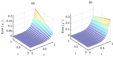
Table 1 show the comparison of the exact solution and the approximate solution obtained by HPM at t = 0:1 and t = 0:3 for any r 2 [0; 1]. Also, in Fig. 1, we compare the exact solution with the approximate solution. The three-dimensional plot of the error between the exact solution and the approximate solution is shown in Fig. 2.
Table 1
The results for six-term approximate of HPM in Example 4.1 case 1.
t = 0:1 t = 0:3
r jy 6j jy 6j jy 6j jy 6j
0 4.5763e-08 2.2875e-07 3.5512e-05 1.7711e-04
0.1 5.4912e-08 2.1960e-07 4.2592e-05 1.7003e-04
0.2 6.4062e-08 2.1045e-07 4.9672e-05 1.6295e-04
0.3 7.3211e-08 2.0130e-07 5.6752e-05 1.5587e-04
0.4 8.2360e-08 1.9215e-07 6.3832e-05 1.4879e-04
0.5 9.1510e-08 1.8300e-07 7.0912e-05 1.4171e-04
0.6 1.0066e-07 1.7385e-07 7.7992e-05 1.3463e-04
0.7 1.0981e-07 1.6470e-07 8.5072e-05 1.2755e-04
0.8 1.1896e-07 1.5556e-07 9.2152e-05 1.2047e-04
0.9 1.2811e-07 1.4641e-07 9.9232e-05 1.1339e-04
0 0.5 1 0
0.5 1 0
5 10
r (a)
t
y−
(t;r)
0 0.5 1 0
0.5 1 0
5 10 15
r (b)
t
y
− (t;r)
Exact solution Approximate solution
Exact solution Approximate solution
Fig. 1. (a) Comparing y(t; r) and 6(t; r) in Example 4.1 case 1. (b) Comparing y(t; r) and 6(t; r) in Example 4.1 case 1.
0 0.5
1 0
0.5 1 0 0.05 0.1 0.15 0.2
t (a)
r
Error ( y
−
)
0 0.5
1 0
0.5 1 0 0.1 0.2 0.3
t (b)
r
Error ( y
− )
Fig. 2. (a) The error of 6(t; r) in Example 4.1 case 1. (b) The error of 6(t; r) in Example 4.1 case 1.
Case (2): If we consider y0(t) in the second form ((ii)-dierentiable), we have to solve
the following dierential system: 8
< :
y0(t; r) = 2 y(t; r) + t2+ 1; y(0; r) = 2 r;
The exact solution is given by 8
< :
y(t; r) = 74e2t+ (r 1)e 2t 1
4(2t2+ 2t + 3);
y(t; r) = 74e2t+ (1 r)e 2t 1
4(2t2+ 2t + 3):
(5.45)
Now, we solve Eq. (44) via HPM and compare approximate solution with exact solution (45).
According to Eqs. (33), (34) and (35), we have
p0: 8 < :
y0(t; r) = 2 r;
y0(t; r) = r; (5.46)
p1 : 8 < :
y1(t; r) = (1 + 2r)t +13t3;
y1(t; r) = (5 2r)t +1
3t3;
(5.47)
and for k 1, we have
pk+1 : 8 > < > :
yk+1(t; r) = 2Rtt0yk(s; r) ds;
yk+1(t; r) = 2Rtt0yk(s; r) ds: (5.48)
We approximate y(t; r) and y(t; r), with 6(t; r) and 6(t; r), respectively, as follows:
6(t; r) = 5 X
i=0
yi(t; r) = r + (5 2r)t + (1 + 2r)t2+ (113 43r)t3+ (12 +23r)t4
+ (1
5 +
11 15r)t5+
1 45t6+
2 315t7;
5(t; r) =X5
i=0
yi(t; r) = (2 r) + (1 + 2r)t + (5 2r)t2+ (1 + 43r)t3+ (116 23r)t4
+ (51 +154 r)t5+451 t6+3502 t7:
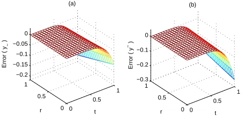
Table 2 show the comparison of the exact solution and the approximate solution obtained by HPM at t = 0:1 and t = 0:3 for any r 2 [0; 1]. Also, in Fig. 3, we compare the exact solution with the approximate solution. The three-dimensional plot of the error between the exact solution and the approximate solution is shown in Fig. 4.
Table 2
t = 0:1 t = 0:3
r jy 6j jy 6j jy 6j jy 6j
0 5.0845e-08 2.2367e-07 4.6676e-05 1.6595e-04
0.1 5.9486e-08 2.1503e-07 5.2640e-05 1.5698e-04
0.2 6.8127e-08 2.0639e-07 5.8603e-05 1.5402e-04
0.3 7.6769e-08 1.9774e-07 6.4567e-05 1.4806e-04
0.4 8.5410e-08 1.8910e-07 7.0530e-05 1.4209e-04
0.5 9.4051e-08 1.8046e-07 7.6494e-05 1.3613e-04
0.6 1.0269e-07 1.7182e-07 8.2458e-05 1.3017e-04
0.7 1.1133e-07 1.6318e-07 8.8421e-05 1.2420e-04
0.8 1.1997e-07 1.5454e-07 9.4385e-05 1.1824e-04
0.9 1.2862e-07 1.4590e-07 1.0035e-04 1.1228e-04
1.0 1.3726e-07 1.3726e-07 1.0631e-04 1.0361e-04
0 0.5
1 0 1 2 0
20 40 60 80
t (a)
r
y−
(t;r)
0 0.5
1 0 1 2 0
20 40 60 80
t (b)
r
y
−(t;r)
Exact solution Approximate solution
Exact solution Approximate solution
Fig. 3. (a) Comparing y(t; r) and 6(t; r) in Example 4.1 case 2. (b) Comparing y(t; r) and 6(t; r) in Example 4.1 case 2.
0 0.5
1 0
0.5 1 −0.2 −0.15 −0.1 −0.05 0
t (a)
r
Error ( y
−
)
0 0.5
1 0
0.5 1 −0.3 −0.2 −0.1 0
t (b)
r
Error ( y
− )
Example 4.2. Consider the following FIVP 8
< :
y0(t) = 3 y(t) et;
y(0) = (r 1; 1 r): (5.49)
Similarly as before, we have two dierent cases.
Case (1): If we consider y0(t) in the rst form ((i)-dierentiable), we have to solve the
following dierential system: 8 < :
y0(t; r) = 3 y(t; r) + et; y(0; r) = r 1;
y0(t; r) = 3 y(t; r) + et; y(0; r) = 1 r: (5.50)
The exact solution of the system is given by 8
< :
y(t; r) = (r 1)e3t 1
4e 3t+ 14et;
y(t; r) = (1 r)e3t 1
4e 3t+ 14et:
(5.51)
Now, we solve Eq. (50) via HPM and compare approximate solution with exact solution (51).
According to Eqs. (28), (29) and (30), we have
p0 : 8 < :
y0(t; r) = r 1;
y0(t; r) = 1 r; (5.52)
p1: 8 < :
y1(t; r) = (et 1) 3(1 r)t;
y1(t; r) = (et 1) 3(r 1)t; (5.53)
and for k 1, we have
pk+1 : 8 > < > :
yk+1(t; r) = 2Rtt0yk(s; r) ds;
yk+1(t; r) = 2Rtt0yk(s; r) ds:
(5.54)
We approximate y(t; r) and y(t; r), with 6(t; r) and 6(t; r), respectively, as follows:
6(t; r) =X5 i=0
yi(t; r) = (r 1) + 61(et 1) + (3r 63)t + (92r 36)t2
+ (92r 272 )t3+ (278 r 274 )t4+ (8140r 8140)t5;
5(t; r) =
5 X
i=0
yi(t; r) = (1 r) + 61(et 1) (3r + 57)t (92r + 27)t2
+ (9
2r + 9 2)t3
27 8 rt4+ (
81 40
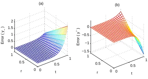
Table 3 show the comparison of the exact and the approximate solution obtained by HPM at t = 0:1 and t = 0:3 for any r 2 [0; 1]. Also, in Fig. 5, we compare the exact solution with the approximate solution. The three-dimensional plot of the error between the exact solution and the approximate solution is shown in Fig. 6.
Table 3
The results for six-term approximate of HPM in Example 4.2 case 1.
t = 0:1 t = 0:3
r jy 6j jy 6j jy 6j jy 6j
0 1.3858e-06 7.2931e-07 1.0723e-03 6.1739e-04
0.1 1.2801e-06 6.2355e-07 9.8785e-04 5.3290e-04
0.2 1.1743e-06 5.1779e-07 9.0336e-04 4.4841e-04
0.3 1.0686e-06 4.1204e-07 8.1888e-04 3.6393e-04
0.4 9.6281e-07 5.0628e-07 7.3439e-04 2.7944e-04
0.5 8.5705e-07 2.0052e-07 6.4991e-04 1.9496e-04
0.6 7.5130e-07 9.4764e-08 5.6542e-04 1.1047e-04
0.7 6.4554e-07 1.0993e-08 4.8093e-04 2.5983e-05
0.8 5.3978e-07 1.1675e-07 3.9645e-04 5.8503e-05
0.9 4.3402e-07 2.2251e-07 3.1196e-04 1.4249e-04
1.0 3.2827e-07 3.2827e-07 2.2748e-04 2.2748e-04
0 0.5 1
0 1 2 −400 −200 0
t (a)
r
y−
(t;r)
Exact solution Approximate solution
0 0.5
1 0
1 2 0 100 200 300 400
r (b)
t
y
−(t;r)
Exact solution Approximate solution
0 0.5
1 0
0.5 1 0 0.5 1 1.5 2
t (a)
r
Error ( y
−
)
0 0.5
1 0
0.5 1 −1.5 −1 −0.5 0
t (b)
r
Error ( y
− )
Fig. 6. (a) The error of 6(t; r) in Example 4.2 case 1. (b) The error of 6(t; r) in Example 4.2 case 1.
Case (2): If we consider y0(t) in the second form ((ii)-dierentiable), we have to solve
the following dierential system: 8
< :
y0(t; r) = 3 y(t; r) + et; y(0; r) = 1 r;
y0(t; r) = 3 y(t; r) + et; y(0; r) = r 1: (5.55)
The exact solution is given by 8 < :
y(t; r) = (r 5
4)e 3t+14et;
y(t; r) = (3
4 r)e 3t+14et:
(5.56)
Now, we solve Eq. (55) via HPM and compare approximate solution with exact solution (56).
According to Eqs. (33), (34) and (35), we have
p0 : 8 < :
y0(t; r) = 1 r;
y0(t; r) = r 1; (5.57)
p1: 8 < :
y1(t; r) = (et 1) 3(1 r)t;
y1(t; r) = (et 1) 3(r 1)t; (5.58)
and for k 1, we have
pk+1 : 8 > < > :
yk+1(t; r) = 2Rtt0yk(s; r) ds;
yk+1(t; r) = 2Rtt0yk(s; r) ds:
We approximate y(t; r) and y(t; r), with 6(t; r) and 6(t; r), respectively, as follows:
6(t; r) =X5 i=0
yi(t; r) = (r 1) + 61(et 1) (3r + 57)t + (9
2r 36)t2
(92r +92)t3+ (27 8 r
27 4 )t4+ (
81 40
81 40r)t5;
5(t; r) =
5 X
i=0
yi(t; r) = (1 r) + 61(et 1) + (3r 63)t + (92r + 27)t2
+ (9
2r 27
2 )t3 27
4 rt4+ ( 81 40r
81 40)t5:
Table 4 show the comparison of the exact solution and the approximate solution obtained by HPM at t = 0:1 and t = 0:3 for any r 2 [0; 1]. Also, in Fig. 7, we compare the exact solution with the approximate solution. The three-dimensional plot of the error between the exact solution and the approximate solution is shown in Fig. 8.
Table 4
The results for six-term approximate of HPM in Example 4.2 case 2.
t = 0:1 t = 0:3
r jy 6j jy 6j jy 6j jy 6j
0 1.2989e-06 6.4242e-07 8.8038e-04 4.2543e-04
0.1 1.2019e-06 5.4535e-07 5.1506e-04 3.6014e-04
0.2 1.1048e-06 4.4828e-07 7.4980e-04 2.9485e-04
0.3 1.0077e-06 3.5121e-07 6.8451e-04 2.2956e-04
0.4 9.1068e-07 2.5414e-07 6.1922e-04 1.6427e-04
0.5 8.1361e-07 1.5707e-07 5.5393e-04 9.8980e-05
0.6 7.1654e-07 6.0007e-07 4.8864e-04 3.3689e-05
0.7 6.1947e-07 3.7062e-07 4.2335e-04 3.1602e-05
0.8 5.2240e-07 1.3413e-07 3.5806e-04 9.6893e-05
0.9 4.2533e-07 2.3120e-07 2.9277e-04 1.6218e-04
1.0 3.2827e-07 3.2827e-07 2.2748e-04 2.2748e-04
0 0.5 1
0 0.5 1 −1 −0.5 0 0.5
r (a)
t
y−
(t;r)
Exact solution Approximate solution
0 0.5
1
0 0.5 1 0 0.5 1
r (b)
t
y
−(t;r)
Exact solution Approximate solution
0 0.5
1 0
0.5 1 0 0.5 1
t (a)
r
Error ( y
−
)
0 0.5
1 0
0.5 1 −0.4 −0.2 0 0.2
t (b)
r
Error ( y
− )
Fig. 8. (a) The error of 6(t; r) in Example 4.2 case 2. (b) The error of 6(t; r) in Example 4.2 case 2.
6 Conclusion
In this paper, we applied Homotopy Perturbation Method (HPM) for approximate solv-ing of the FIVP. The original FIVP is replaced by two parametric ordinary dierential equations which are then solved approximately using the HPM. HPM provides the com-ponents of the exact solution, where these comcom-ponents should follow the summation give in (21). The exact solutions are compared with solutions obtained by means of the HPM. The results show that this method is useful for nding an accurate approximation of the exact solution. Also, this method can be used for solving N-th fuzzy dierential equations.
References
[1] S. Abbasbandy, T. Allahviranloo, Numerical solutions of fuzzy dierential equations by taylor method, Computational Methods in Applied Mathematics 2 (2002) 113{124.
[2] S. Abbasbandy, T. Allahviranloo, O. Lopez-Pouso, J.J. Nieto, Numerical methods for fuzzy dierential inclusions, Computer and Mathematics With Applications 48/10-11 (2004) 1633{ 1641.
[3] T. Allahviranloo, N. Ahmady, E. Ahmady, Numerical solution of fuzzy dierential equations by predictorcorrector method, Information Sciences 177/7 (2007) 1633{1647.
[4] T. Allahviranloo, E. Ahmady, A. Ahmady, N-th fuzzy dierential equations , Information Sciences 178 (2008) 1309{1324.
[5] G.A. Anastassiou, S.G. Gal, On a fuzzy trigonometric approximation theorem of Weierstrass-type, J. Fuzzy Math. 9 (3) (2001) 701{708.
[7] B. Bede, I. Rudas, A. Bencsik, First order linear fuzzy dierential equations under generalized dierentiablity, information secieness 177 (2006) 3627{3635.
[8] B. Bede, S. G. Gal, Generalizations of the dierentiability of fuzzy-number-valued functions with applications to fuzzy dierential equations, Fuzzy Sets and Systems 151 (2005) 581{599.
[9] Y. Chalco-Cano, H. Roman-Flores, On new solutions of fuzzy dierential equations, Chaos, Solitons and Fractals (2006) 1016{1043.
[10] S.S.L. Chang, L. Zadeh, On fuzzy mapping and control, IEEE Trans. Systems Man Cybernet. 2 (1972) 30{34.
[11] D. Dubois, H. Prade, Towards fuzzy dierential calculus, Fuzzy Sets and Systems 8 (1982) 1{7 , 105{116, 225{233.
[12] M. Friedmen, M. Ming, A. Kandel, Fuzzy derivatives and fuzzy Cauchy problems using LP metric, in: Da Ruan (ED.), Fuzzy Logic Foundations and Industrial Applications, Kluwer Dordrecht, 1996, pp.57{72.
[13] S.G. Gal, Approximation theory in fuzzy setting, in: G.A.Anastassiou (Ed.), Handbook ofAnalytic-Computational Methods in Applied Mathematics, Chapman & Hall/CRC, Boca Raton, London, NewYork,Washington DC, 2000, pp. 617{666.
[14] R. Goetschel, W. Voxman, Elementary calculus, Fuzzy Sets and Systems 18 (1986) 31{43.
[15] O. He. W. Yi, On fuzzy dierential equations, Fuzzy Sets and Systems 24 (1989) 321{325.
[16] J.H. He, A coupling method of a homotopy technique and a perturbation technique for non-linear problems. International Journal of Non-Linear Mechanics 35 (1) (2000), 37{43.
[17] J.H. He, Application of homotopy perturbation method to nonlinear wave equations, Chaos, Solitons and Fractals 26 (2005) 695{700.
[18] J.H. He, Homotopy perturbation method for solving boundary value problems, Physics Letters A 350 (2006)87{88.
[19] J.H. He, Limit cycle and bifurcation of nonlinear problems, Chaos, Solitons and Fractals 26 (3) (2005) 827{833.
[20] J.H. He, The homotopy perturbation method for nonlinear oscillators with discontinuities, Applied Mathematics and Computation 151 (2004) 287{292.
[21] A. Kandel, M. Friedmen, M. Ming, On Fuzzy dynamical processes, Proc. FUZZ-IEEE'96, New Orleans, 8{11 Sept. 1996, pp. 1813{1818.
[22] O. Kaleva, Fuzzy dierential equations, Fuzzy Sets Systems 24 (1987) 301{317.
[23] O. Kaleva, The Cauchy problem fo fuzzy dierential equations, Fuzzy Sets Systems 35 (1990) 389{396.
[25] W. Menda, Linear fuzzy dierential equation systems on R1, Jounal of Fuzzy Systems Math-ematics 2 (1) (1988) 51{56, in Chinese.
[26] M.L. Puri, D. Ralescu, Dierential for fuzzy function, J. Math. Anal. Appl. 91 (1983) 552{558.
[27] S. Seikkala, On the fuzzy initial value problem, Fuzzy Sets and Systems 24 (1987) 319{330.
![Table 1 show the comparison of the exact solution and the approximate solution obtainedby HPM at t = 0:1 and t = 0:3 for any r 2 [0; 1]](https://thumb-us.123doks.com/thumbv2/123dok_us/8879086.1818660/11.612.96.469.485.668/table-comparison-exact-solution-approximate-solution-obtainedby-hpm.webp)
![Table 2 show the comparison of the exact solution and the approximate solution obtainedby HPM at t = 0:1 and t = 0:3 for any r 2 [0; 1]](https://thumb-us.123doks.com/thumbv2/123dok_us/8879086.1818660/13.612.102.510.447.594/table-comparison-exact-solution-approximate-solution-obtainedby-hpm.webp)
![Table 3 show the comparison of the exact and the approximate solution obtained by HPMat t = 0:1 and t = 0:3 for any r 2 [0; 1]](https://thumb-us.123doks.com/thumbv2/123dok_us/8879086.1818660/16.612.194.420.457.578/table-comparison-exact-approximate-solution-obtained-hpmat-t.webp)
![Table 4 show the comparison of the exact solution and the approximate solution obtainedby HPM at t = 0:1 and t = 0:3 for any r 2 [0; 1]](https://thumb-us.123doks.com/thumbv2/123dok_us/8879086.1818660/18.612.96.464.369.549/table-comparison-exact-solution-approximate-solution-obtainedby-hpm.webp)

