Mixed Variational-Monte Carlo Assimilation of Streamflow Data in Flood Forecasting: the Impact of Observations Spatial Distribution

(1)

Engineering

EPiC Series in Engineering

Volume 3, 2018, Pages 668–675

HIC 2018. 13th International Conference on Hydroinformatics

Mixed Variational-Monte Carlo Assimilation of Streamflow

Data in Flood Forecasting: the Impact of Observations

Spatial Distribution

Giulia Ercolani

1

_{and Fabio Castelli}

1

Department of Civil and Environmental Engineering, University of Florence, Florence, Italy

[email protected], [email protected]

Abstract

A mixed variational-Monte Carlo scheme is employed to assimilate streamflow data at multiple locations in a distributed hydrologic model for flood forecasting purposes. The goal of this work is to assess the role of the spatial distribution of the assimilation points in terms of forecasts accuracy. The area of study is Arno river basin, and the strategy of investigation is to focus on one single nearly-flood event, performing various assimilation experiments that differ only in number and location of the assimilation sites.

1 Introduction

(2)

Figure 1: Scheme of the mixed variational-Monte Carlo assimilation method (from [3]).

where the only varying characteristics are the number and location of the assimilation sites. We evaluate the impact on the forecasted river flow at both the assimilated and not assimilated points.

2 The Hydrologic Model

The assimilation system is developed for the physically based and spatially distributed hydro-logic model MOBIDIC (MOdello di Bilancio Idrohydro-logico DIstribuito e Continuo) [1,4,5], which is employed operatively at the hydrologic service of Tuscany region (Servizio Idrologico Regionale, Regione Toscana) for floods forecasting and water resources management purposes. The basic characteristics of MOBIDIC are: i) a raster-based discretization of the watershed, ii) a vector-based representation of the hydrographic network, iii) a detailed and computationally efficient representation of soil moisture dynamics [2], iv) a modular structure which allows to tune the level of complexity of the represented processes for each specific application. In the present case, we adopt the setting employed in [3], i.e. the cascade of linear reservoirs for flow routing through the river network and the linear conceptual reservoir for groundwater dynamics.

3 The Mixed Variation-Monte Carlo Assimilation System

(3)

Observations Spatial Distribution in Streamflow Data Assimilation G. Ercolani and F. Castelli

equation for streamflow is:

dQ(t)

dt =A[qL(t) +U Q(t)−Q(t)] =F(A,Q(t),qL(t)) (1)

where, considering a network composed bynreaches, Q(t)∈Rn are flows exiting each reach, qL(t)∈Rn are lateral inflows to each reach (surface runoff plus groundwater flow), and A∈ Rn×n is a diagonal matrix containing the inverse of the characteristic residence time of each

reach on the diagonal. Lastly,U ∈Rn×n is a binary matrix accounting for network topology.

The adjoint model of (1) is derived by minimizing a penalty functionalJ containing squared errors between modelled and observed river flows, and between current and previous values of the quantities to optimize, while physically constrained by ( 1) through a vector of Lagrange multipliersλ(t)∈_Rn_{. The quantities to optimize are the initial flow in each river reach}_Q

0, and

the time series of the later inflowqL. After some computations, the minimization ofJ leads

to a system of ordinary differential equations that describes the time evolution of Lagrange multipliers λ. Furthermore, a terminal condition for the backward integration of the adjoint model, as well as update equations for initial streamflow Q0 and lateral input qL depending

onλ(t) are obtained. An iterative procedure constituted by subsequent integrations of forward and adjoint model, and corresponding updates of Q0 and qL, provides optimal estimates of

Q0 and qL. It is important to underline that a mismatch between observed and modelled Q

at a specific location perturbs λ not only locally, but also in the upstream reaches. This is due to the coupling existing between the equations for flow channel routing (see eq. (1)), and allows to spread the updates of Q0 and qL throughout the upstream portion of the network.

The equations composing the adjoint model and the detailed steps to obtain it can be found in [3]. SinceqL is a state variable of MOBIDIC model, mass conservation is not guaranteed

if it is updated indiscriminately. It is dependent on runoff formation and hillslope routing, as well as on groundwater dynamics through base flow. All these phenomena should be included as physical constraints in the minimization of the functional J. However, this strategy would be unpractical, especially because of the numerous threshold processes characterizing runoff formation. A more effective approach is to combine the just described variational approach with a parsimonious Monte Carlo technique. Namely, we infer key quantities for runoff formation on the basis of both an ensemble ofqL and optimal estimates from the variational procedure. In

practice, the steps of the strategy are the following. First, we generate an ensemble ofqLonce

at the beginning of the assimilation by reasonably varying a couple of fundamental quantities in terms of runoff formation (i.e. initial soil moisture and rainfall intermittence). Both variables are maintained spatially homogeneous, so that the size of the ensemble remains small (typically around 100 realizations). Then, we run an iteration of the variational procedure to updateqL

time series on the basis of the mismatch between observed and modelled river flows during the assimilation window. Finally, for any single river reach independently and at each iteration, we “pick up”the realization ofqL in the predetermined ensemble which is the most similar to

the variational estimate. Initial soil moisture and rainfall intermittence corresponding to the selected realization are adopted for the cells contributing to the corresponding reach. Hence, a spatially distributed estimate of both quantities is obtained. Figure1describes the assimilation strategy schematically.

4 Assimilation Experiments

(4)

Figure 2: Arno river network and location of the 25 observation points.

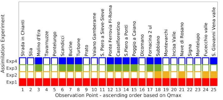
Figure 3: Summary of the assimilation sites in each experiment: rows correspond to experi-ments, columns to streamflow observation points; the cell is filled if observations are assimilated.

experiments which differ only in number and location of the assimilation points. All the simu-lations employ a spatial resolution of 500 m and a time step of 15 minutes. The extent of each assimilation window is 6 hours.

4.1 Area of Study and Data

The assimilation experiments are performed in the Arno river basin (central Italy, about 8300 km2_{), whose mainstream is about 240 km length. The simulated event is selected among those}

(5)

ob-Observations Spatial Distribution in Streamflow Data Assimilation G. Ercolani and F. Castelli

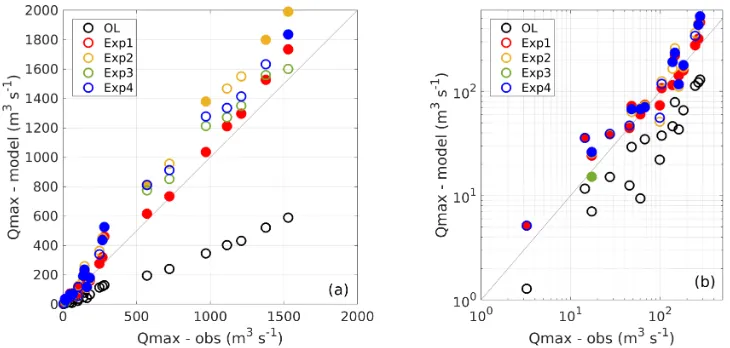
Figure 4: Scatter plots (a - linear scale, b – zoom in logarithmic scale) of peak flow at the 25 observation points for Open Loop (OL, black circles), 1st _{Assimilation Experiment (Exp1,}

red circles), 2nd _{Assimilation Experiment (Exp2, yellow circles), 3}rd _{Assimilation Experiment}

(Exp3, green circles), and 4th _{Assimilation Experiment (Exp4, blue circles). Circles are filled}

if streamflow observations are assimilated at the corresponding location.

servations are available only at 5 locations along the mainstream, secondly, in order to focus on the role of assimilation points spatial distribution, we want to avoid disturbances due to both specific characteristics of the event that the model could not represent, and uncoherent observations at the various sites. In particular, synthetic observations are discharge time series extracted from a run of MOBIDIC model, started 13 days before the period of interest, and initialized with a map of soil moisture including both saturated and nearly dry areas. Employ-ing synthetic data potentially allows to have at disposal observations at any desired location. However, we prefer to locate the synthetic measurement stations in correspondence of real hy-drometers in the network (Figure 2). The experiments assimilates data from: i) all the 25 synthetic stations of Figure 2 (baseline assimilation run, 1st assimilation experiment), ii) the 5 stations along the mainstream employed in [3], i.e. Subbiano, Montevarchi, Nave di Rosano, Fucecchio, San Giovanni alla Vena (2nd Assimilation Experiment), iii) the stations placed in proximity of the outlet of the main tributaries (3rd Assimilation Experiment), iv) the stations placed close to the outlet of the main tributaries plus San Giovanni alla Vena (4th Assimilation Experiment). This rationale is summarized in Figure3, where, for each location of Figure 2, it is specified whether data are actually assimilated (filled square) or not (empty square) during each experiment. The 25 synthetic measurement stations are reported in ascendant order, to facilitate the interpretation of the results shown in Section 5. All the experiments include 5 sequential assimilation windows, corresponding to 30 hours of observations. The results shown in Section5 refer to the final assimilation window for all the experiments.

5 Results

(6)

at the 25 locations of interest, with the plot on the left in linear scale (a), and the zoom on the right in logarithmic scale (b), in order to present the behaviour also in reaches with lower discharges. All the experiments predict the peak flow more accurately than the open loop run (OL, black circles) at any observation point. The best performances are obtained with the 1st

experiment (Exp1, red circles), i.e. when streamflow data are assimilated at all the displayed locations. However, especially for the larger peak flows, the performances are not directly related to whether data are or are not assimilated locally. In fact, for both Fucecchio (the second highest peak flow) and Nave di Rosano (the fifth highest peak flow) a more accurate forecast is obtained in the 3rd and 4th experiments (green and blue circles), not assimilating data locally, than in the 2nd one (yellow circles), which assimilates streamflow observations at both these locations. Furthermore, at San Giovanni alla Vena (the highest peak flow), the best prediction corresponds to the 3rd _{experiment, which is the only one not assimilating locally.}

Overall, the 3rd _{experiment provides results similar to those of the full assimilation (Exp1)}

at many locations. Since the 3rd _{experiment assimilates data in proximity of the outlet of}

the main tributaries of Arno river, it can be stated that an assimilation employing a lower number of assimilation points may perform comparably to one using more stations, provided that the spatial distribution of the points is hydrologically meaningful. The 4th _experiment

differs from the 3rd _{one only in assimilating data also at S. Giovanni alla Vena in addition to}

the main tributaries. Nevertheless, performances are generally worse, especially for the higher peak flows. This fact suggests that the assimilation updates may deteriorate if the magnitude of the employed data differs significantly among the assimilation points, as it happens in the 4th experiment in respect to the 3rd one (i.e. the observed discharges in the tributaries are much lower than those at S. Giovanni alla Vena). The less accurate forecasts are obtained in the 2ndexperiment, outperformed by the 3rdand 4thtests also at its owns assimilation points. The reason is probably twofold. Firstly, the number of assimilation point is extremely low (only 5), corresponding to a very high degree of freedom in the inverse problem. Secondly, the magnitude of the assimilated data is significantly lower at 2 of the 5 assimilation points (at Subbiano and Montevarchi, with an observed peak of about 280 and 570 m3_s−1_{, in respect to}

Nave di Rosano, Fucecchio and S. Giovanni, with maximum streamflows of about 970, 1400 and 1500 m3_s−1_{). As previously noticed, the effectiveness of assimilation points whose data are}

much lower than the others employed is limited. This means that the 2nd_{experiment essentially}

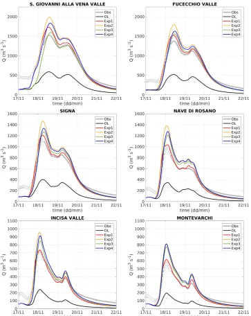
relies on only 3 points. In order to further clarify the obtained results, Figure5shows the full hydrograph corresponding to the open loop and the 4 assimilation experiments at 6 selected stations, all located along the main stream of Arno river. The hydrographs are displayed from downstream to upstream, with S. Giovanni alla Vena being the point closest to the outlet. It is immediately visible that the full assimilation (Exp1) provides the best results if both the timing and magnitude of the discharges are considered, and that the most comparable results are obtained with the 3rd experiment, although with slightly worse performances.

6 Conclusions

(7)

Observations Spatial Distribution in Streamflow Data Assimilation G. Ercolani and F. Castelli

Figure 5: Hydrographs at 6 selected locations along the main stream of Arno river for the open loop and the 4 assimilation experiments (line colours maintain the same meaning of Figure4), and with observations in grey (triangles are the assimilated observations, in case the experiment includes assimilation at the shown location).

(8)

supplementary point, whose data are much greater than the other employed, may even worsen the performances. This behaviour is connected to the rationale of the assimilation scheme, based on the adjoint model of the flow routing throughout the river network and hence maintaining the coupling between connected reaches. Hence, one of the main advantages of the system, i.e. the capability of spreading updates upstream of an assimilation point naturally, may represent also a vulnerability if the assimilation sites are not selected properly.

References

[1] Fabio Castelli, Giovanni Menduni, and Bernardo Mazzanti. A distributed package for sustainable water management: a case study in the Arno basin. IAHS Publ., 327:52–61, 2009.

[2] Aldrich Castillo, Fabio Castelli, and Dara Entekhabi. Gravitational and capillary soil moisture dynamics for distributed hydrologic models. Hydrology and Earth System Sciences, 19(4):1857, 2015.

[3] Giulia Ercolani and Fabio Castelli. Variational assimilation of streamflow data in distributed flood forecasting. Water Resources Research, 53(1):158–183, 2017.

[4] Jing Yang, Fabio Castelli, and Yaning Chen. Multiobjective sensitivity analysis and optimization of distributed hydrologic model mobidic. Hydrology and Earth System Sciences, 18(10):4101–4112, 2014.