R E S E A R C H
Open Access
Dynamic linear models guide design and
analysis of microbiota studies within
artificial human guts
Justin D. Silverman
1,2,3, Heather K. Durand
5, Rachael J. Bloom
4, Sayan Mukherjee
1,6and Lawrence A. David
1,3,4,5*Abstract
Background:Artificial gut models provide unique opportunities to study human-associated microbiota.
Outstanding questions for these models’fundamental biology include the timescales on which microbiota vary and the factors that drive such change. Answering these questions though requires overcoming analytical obstacles like estimating the effects of technical variation on observed microbiota dynamics, as well as the lack of appropriate benchmark datasets.
Results:To address these obstacles, we created a modeling framework based on multinomial logistic-normal dynamic linear models (MALLARDs) and performed dense longitudinal sampling of four replicate artificial human guts over the course of 1 month. The resulting analyses revealed how the ratio of biological variation to technical variation from sample processing depends on sampling frequency. In particular, we find that at hourly sampling frequencies, 76% of observed variation could be ascribed to technical sources, which could also skew the observed covariation between taxa. We also found that the artificial guts demonstrated replicable trajectories even after a recovery from a transient feed disruption. Additionally, we observed irregular sub-daily oscillatory dynamics associated with the bacterial family Enterobacteriaceae within all four replicate vessels.
Conclusions:Our analyses suggest that, beyond variation due to sequence counting, technical variation from sample processing can obscure temporal variation from biological sources in artificial gut studies. Our analyses also supported hypotheses that human gut microbiota fluctuates on sub-daily timescales in the absence of a host and that microbiota can follow replicable trajectories in the presence of environmental driving forces. Finally, multiple aspects of our approach are generalizable and could ultimately be used to facilitate the design and analysis of longitudinal microbiota studies in vivo.
Keywords:Artificial gut, Bioreactor, Microbiome, Metagenomics, Compositional data, Bayesian statistics, Time series analysis
Background
Artificial gut models have been used for decades to repli-cate the human intestinal environment and study the dy-namics of resident microbes [1–3]. These systems have the advantage of being sampled with arbitrary frequency, house environments that can be precisely controlled, and often face fewer ethical concerns than in-human
studies [4]. Artificial gut models have therefore been used to discover the effect of nutritional supplements on infant gut microbiota [5], mechanisms by how commensals re-press Salmonella virulence [6], and dose-dependencies between microbiota-targeting therapies and metabolite production [7].
Yet, despite the utility and long development of artificial gut models, fresh questions regarding their fundamental biology remain. Such questions include the rapidity with which the composition of these microbial communities varies both in the presence and absence of perturbations [1,8]. While it is well known that in vivo microbiota may change on sub-daily timescales due to host forcing, it is * Correspondence:[email protected]
1
Program in Computational Biology and Bioinformatics, Duke University, CIEMAS, Room 2171, 101 Science Drive, Box 3382, Durham, NC 27708, USA 3Center for Genomic and Computational Biology, Duke University, Durham,
NC 27708, USA
Full list of author information is available at the end of the article
unclear whether such sub-daily dynamics may be seen in the absence of host effects [9]. The degree to which replicate ex vivo systems exhibit stochastic behavior, or conversely behave deterministically, remains another outstanding question [1, 10]. Finally, a deeper under-standing of the reproducibility of artificial gut models may also have implications for our understanding of the relative importance of various factors in shaping the dynamics of host-associated microbiota [11].
Gaining greater insight into the biology of artificial gut models though requires addressing analytical and statis-tical challenges. One key challenge is the often unquanti-fied impact of artificial sources of intra-study variation such as variation due to sequencing counting and tech-nical variation from sample processing (e.g., unintended experimental errors and batch effects) [12–18]. In particu-lar, while the impact of variation due to sequence counting is more commonly addressed and modeled [12,19–21], the impact of technical variation from sample processing is often unquantified and less well understood. Such technical variation may alter inference of both the magnitude and direction of variation among bacterial taxa. In addition, it is well established that sequencing studies of microbiota pro-vide information only on the relative amounts of taxa and not their absolute abundance [22–24]. The analysis of such relative (or compositional) data remains an open area of study and naive analyses can lead to a distorted view of the patterns of variation present in a commu-nity [21, 22, 25–27]. Notably, the variation due to se-quence counting, technical variation from sample processing, and compositional effects are all challenges facing in vivo microbiota studies, in addition to artifi-cial gut experiments.
The design of ex vivo microbiota studies is also con-fronted by the lack of appropriate benchmark datasets. For example, defining suitable sampling frequencies for artificial gut studies requires insight into the timescales on which human gut microbiota fluctuate [28]. Yet, even though gut microbiota dynamics in vivo and bacterial mock communities in vitro are known to behave on the timescale of hours [9,29,30], most longitudinal studies to date in ex vivo models are only sampled on the order of days [1, 8, 10, 31]. Additionally, while the collection of technical replicates could be used to quantify the effects of technical variation [32], such replicate sampling is gen-erally not performed in longitudinal microbiota studies.
Here, we integrated model development and experimen-tal design to address key challenges facing the analysis and design of longitudinal artificial gut studies. We collected longitudinal samples with up to hourly frequency from replicate artificial gut models over the course of 1 month. We combined this longitudinal sampling with the collec-tion of technical replicates so that we could characterize the impact of technical sources of variation on observed
microbiota dynamics. To isolate separate biological and technical sources of community variation in our dataset, we created a modeling framework called MALLARD that is based on a class of generalized dynamic linear models appropriate for microbiota time-series data. Together, our dataset and modeling framework allowed us to investigate the patterns and timescales of microbiota variation in an artificial human gut.
Results
Longitudinal modeling
To separate biological and technical variation in artificial gut time-series, we introduce an extension of dynamic lin-ear models (DLMs) tailored for microbiota data. DLMs have widespread use including industrial applications such as commercial forecasting and engineering control sys-tems [33]. At their core, DLMs model a system as a time-varying state that is observed through a noisy process. We extended DLMs to a class of multinomial logistic-normal dynamic linear models by building off of the work by Cargnoni C, Muller P, and West M [34]. We refer to this as the MALLARD class of models.
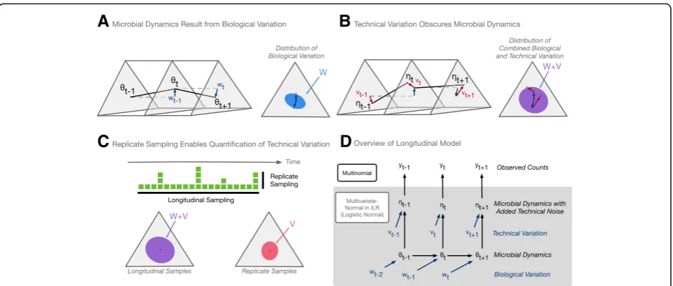
We analyzed the artificial gut dataset described below using a MALLARD model that is generative and as-sumes there exists an unobserved microbial composition (θt; the state) that evolves through time (Fig.1a) due to
stochastic biological variations (wt). We regard the state
sequence (θ1,…,θt,…,θT) as the true microbial
dynam-ics in a time-series. Random technical variations (vt) are
then added to the true system state (θt) resulting in the
compositionηt(Fig.1b). We observeηtthrough a
multi-nomial counting process. This formulation is similar to the constant level model commonly used in Bayesian time-series analysis [34]. By separately modeling the process generating wt and vt with distinct covariance
matrices (W and V, respectively), we can decouple bio-logical and technical variations in artificial gut datasets (Fig. 1c). Visually, we found this model provided a good fit to artificial gut data (Additional file1).
Daily and hourly gut microbiota time-series in an artificial human gut
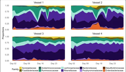
We applied our model to an artificial gut that was con-structed using continuous-flow anaerobic bioreactor systems that have been validated as models of human gut microbiota [1, 6,14,35,36]. The same starting human fecal inoculum was seeded into replicate ex vivo vessels (n= 4) and cultured for 1 month (Fig. 2 and Additional files 2, 3, 4, and 5). Throughout the experiment, pH, temperature, media input rates, and oxygen concentration were all fixed (“Methods”
section). To introduce microbial dynamics into our systems, a single bolus ofBacteroides ovatus isolated from the stool donor was administered to the system on Day 23 (“Methods”
on microbial dynamics, but the media it was suspended in appeared to induce minor shifts in the relative abundances of select bacterial taxa that were visible with hourly sampling (Additional file3). Additional microbial dynamics related to media input were generated by an inadvertent feed disrup-tion in two vessels between days 11 and 13 of the study. Overall, similar to previous studies [1,10], the artificial gut maintained much of the microbial diversity present in the in-oculating stool: 91% of bacterial families present on days 1–5 of the study were detected between days 23 and 28. The 9% of bacterial families that did not persist represented only 0.06% of the total sequencing reads in the dataset.
To investigate the timescales on which microbial com-munities vary ex vivo and to characterize the impact of technical variation on our measurements, we developed a sampling scheme for our artificial gut that featured fine temporal resolution and numerous technical repli-cates (Additional file4). As in previous studies, all four vessels of the artificial gut were sampled daily over the course of 1 month. To investigate potential sub-daily variation, we aimed to oversample the system and col-lected 120 sequential hourly samples, from each repli-cate vessel, during a 5-day period. To estimate the technical variation in our measurements, we collected 20 replicate samples from the final time-point of each artificial gut vessel (Fig. 1c; “Methods” section). As
samples collected in the same vessel at the same time are expected to be biologically identical (i.e., feature no biological variation), any variation in the resulting com-munity measurements between these technical replicates can be ascribed solely to technical sources (Fig. 1c). To ensure that the technical variation profile of the replicate sampled matched that of the longitudinal samples, all samples were randomized and processed together for sequencing.
The structure and magnitude of technical variation from sample processing
After fitting the MALLARD model to the resulting arti-ficial gut dataset, we investigated the technical variation from sample processing (V) to our inference of variation due to biological sources (W). Variation from sample processing and variation due to sequence counting were represented as separate processes (Fig.1d). Differing cor-relation structure between Vand W would support our hypothesis that sources of technical variation could ob-scure biological forces acting on microbiota within an artificial gut. Indeed, a permutation analysis indicated it highly improbable that V and W had the same correl-ation structure (posterior probability < 1%; “Methods”
section). Low-dimensional projections of the posterior distributions ofVand W supported this conclusion and
A
C
D
B
revealed how overall variation patterns involving bacter-ial families like Lachnospiraceae, Fusobacteriaceae, and Bacteroidaceae more strongly resembled patterns of technical variation than biological variation (Fig. 3a). Thus, some patterns of covariation among taxa in artifi-cial gut studies may be due to technical sources of variation.
We next investigated the relative magnitude of tech-nical variation from sample processing and biological variation as a function of sampling frequency. Total vari-ation is defined as the trace of a covariance matrix [37]. We therefore computed Tr(W)/Tr(V), which is analo-gous to the signal-to-noise ratio used in signal process-ing [38]. We found that for our time-series analyzed on an hourly basis (“Methods”section), the median ratio of biological to technical variation was 0.30 (0.26–0.36 95% credible interval). We therefore estimate that only 24% (21%–26%) of the total variation in relative abundances was due to biological sources. This result was insensitive to perturbation of our priors (Additional file 6). Moreover, because variance is additive between time-points within our model, we could estimate bio-logical and technical variation as a function of sampling
interval (Fig.3b;“Methods” section). We found that at a sampling interval of 3.5 h, the total biological and tech-nical variation was approximately equal. At sampling frequencies faster than 3.5 h, technical variation out-weighed biological variation; at slower sampling frequen-cies, signal associated with biological variation exceeded technical noise.
Timescales of microbial dynamics
In order to explore the timescale of microbial dynam-ics within replicate artificial gut vessels, we visualized microbial dynamics using PhILR balances. PhILR bal-ances represent the log-ratio between phylogenetically neighboring clades of taxa, providing a phylogenetic-ally informed way to study microbial dynamics with-out compositional artifacts [22]. We quantified the magnitude of changes in balance values in units of evidence information (e.i.), which are a measurement of compositional change [39]. A 1 e.i. change is equivalent to an approximately 4-fold change in the ratio of two bacterial taxa and a 2 e.i. change is equivalent to an approximately 17-fold change in the ratio of two taxa (see “Methods” section for further
discussion). Multiple balances exhibited sub-daily dy-namics (Additional files 7 and 8), most notably the ratio of bacteria from the phylum Bacteroidetes to bacteria from the phyla Proteobacteria and Fusobac-teria (Fig. 4). The balance between Bacteroidetes and Proteobacteria/Fusobacteria appeared to fluctuate on timescales shorter than 1 day with an amplitude of approximately 1 e.i. (0.5–1.5, 95% credible interval; Fig. 4b). Balance dynamics did not correspond to re-corded environmental or technical variations (e.g., media changes, identity of the researcher collecting the sample, sequencing batch number, B. ovatus supple-mentation, or the feed disruption of vessels 1 and 2) and did not display an exact 24-h periodicity (Additional file9). Balance fluctuations were observed in all four replicate artificial gut models, but did not appear to be synchro-nized as would be expected if these dynamics were driven by a shared environmental factor (Additional file 8). We ultimately could not identify a technical or environmental cause of fluctuating balance dynamics on sub-daily timescales.
Exploratory analysis of biological variation
We next explored the biological variation captured in our model by investigating the pairwise variation between bac-terial families in our dataset. Direct taxon-level analysis of the covariance matrixWis difficult though because the el-ements of this matrix are balances—not individual taxa. We therefore investigated the temporal variation of spe-cific taxon pairs using a tool from compositional data ana-lysis called the variation array [40]. A variation array represents the variance of the log-ratio between pairs of
B
A
Fig. 3Structure and magnitude of biological and technical variation.
aTernary plot showing the 95% probability regions of the logistic-normal distributions corresponding toW,V, andW+Valong the Bacteroidaceae, Fusobacteriaceae, and Lachnospiraceae subcomposition. To visualize posterior uncertainty, 100 posterior samples of each of these quantities are plotted.bMean and 95% credible interval for total biological (Tr(W)) and total technical (Tr(V)) variation as a function of sampling interval in hours
A
B
taxa (“Methods” section). When variance of a pairwise log-ratio is near zero, the two taxa positively covary; whereas when this variance is, high the two taxa exhibit either unlinked or exclusionary patterns [22, 41]. The resulting variation array (corresponding to W) revealed that most temporal variation was contained in log-ratios between four bacterial families: the Rikenellaceae, Syner-gistaceae, Enterobacteriaceae, and Fusobacteriaceae. By contrast, log-ratios between other bacterial families were approximately 1 order of magnitude smaller (Fig. 5a). Overall, we estimated that the Rikenellaceae, Synergista-ceae, EnterobacteriaSynergista-ceae, and Fusobacteriaceae accounted for 72% (69–75%; CLR basis) of the total biological vari-ation seen in the dataset (Additional files10and11).
We noticed an inverse relationship between the bio-logical variation of taxa to their relative abundance in the starting inoculum. We observed this relationship by fitting a linear regression model to each posterior sample in a CLR-transformed space (95% posterior credible interval for regression slope: −0.26 to −0.18; Additional file 12; “Methods” section). Thus, our ana-lyses suggested that more variable taxa in the artificial gut tended to be rarer at the time of inoculation. This result was insensitive to perturbation of our prior assumptions (Additional file 13), and there was only a 3.8% posterior probability that the observed in-verse relationship was an artifact of low abundance
families being more numerous than high abundance ones (“Methods” section).
To better understand the patterns of variation we ob-served from the above analysis, we manually created three balances which together highlighted patterns that we believe explain the high variability of the Rikenella-ceae, SynergistaRikenella-ceae, EnterobacteriaRikenella-ceae, and Fusobac-teriaceae families (Fig. 5b–d). Together, these three manually curated balances explained 73% of the bio-logical variation in the dataset (69–76%, 95% credible interval). This manual curation was informed by the in-spection of microbial dynamics within the PhILR basis and a hierarchical cluster analysis which suggested that the Fusobacteriacae and Synergistaceae shared similar dynamic patterns and should therefore be grouped to-gether for analysis (“Methods” section, Additional file
14). One highly variable balance, which represented the ratio of Rikenellaceae to the other nine bacterial families, exhibited a 3e.i. decrease during days 11–13 in two arti-ficial gut replicate vessels before recovering over the subsequent week (Fig. 5b). This decrease corresponded with the transient feed disruption in those replicate ves-sels. A second highly variable balance, the ratio between the Fusobacteriaceae and Synergistaceae to all other bac-terial families, increased by approximately 8e.i. between days 2 and 7 and the end of the experiment (Fig. 5c). The nadir of this balance coincided with an initial
A
B
C
D
Fig. 5The decomposition of biological variation among bacterial families.aHeatmap of posterior distribution of log-ratio variance (ρ) between pairs of bacterial families. Heatmap color is given by the median of the posterior distribution ofρ. Columns and rows refer to the bacteria in the numerator and denominator of the corresponding log-ratios respectively. A similar decomposition of technical variation is shown in
microbiota adaptation phase that is repeatedly reported in artificial gut studies [1, 10]. A third balance, repre-senting the ratio of Enterobacteriaceae to the other nine bacterial families, exhibited irregular sub-daily oscillatory behavior (Fig.5d and Additional file 15). These balance dynamics are likely related to those observed earlier between the phyla Bacteriodetes and Fusobacteria/Pro-teobacteria (Fig.4), given the membership of Enterobac-teriaceae within the phylum Proteobacteria.
Discussion
Our findings in concert offer several insights that could be useful for the design and analysis of ex vivo studies of human gut microbiota. Our study suggests that technical variation introduced during sample processing can affect observations of microbiota dynamics not just in scale but also in the patterns of covariation among taxa. To date, knowledge has been limited on the effects of tech-nical variation in ex vivo studies of human gut micro-biota. Select exceptions include prior bioreactor studies that found technical variation to be limited and domi-nated by biological variation [10].
Our methods and results also have implications for the choice of sampling frequency in ex vivo artificial gut studies. While oversampling can waste resources, under-sampling can bias inference through a mechanism known as signal aliasing [28, 42, 43]. Here, to balance between resource-intensive exploration of sub-daily dynamics while still capturing longer multi-day dynamics, we made use of MALLARD and mixed rate sampling (e.g., sampling at both daily and hourly timescales). Our findings suggest that future studies interested in tracking the full range of ex vivo micro-biota dynamics or that focus on community responses to rapidly changing external factors (e.g., single dose small mol-ecule or prebiotic supplementation studies) should consider collecting sub-daily measurements. By contrast, studies inter-ested solely in longer term changes (e.g., overall nutritional studies) may find daily sampling sufficient. Additionally, by combining replicate sampling with purposeful oversampling, we were able to determine an effective signal-to-noise ratio as a function of sampling frequency. This ratio could be used to estimate an upper-limit sampling frequency above which the benefits of increases samples are diminished by the rela-tively high levels of technical variation.
Another methodological approach we develop here for artificial gut studies is an exploratory technique for dis-covering temporal patterns among microbial taxa. As gut microbiota time-series often involve many taxa, methods of dimension reduction can aid data interpret-ation. Yet, many standard time-series tools for dimen-sion reduction, such as dynamic principal component analysis, are not well suited for microbiota data in the form of relative taxa abundances. We overcome this challenge and identify distinct patterns in our dataset
using a tool from compositional data analysis called the variation array [40]. Hierarchical cluster analysis and manual curation then allowed us to identify three bal-ances (Fig. 5b–d), highlighting four bacterial families, that together accounted for over 70% of the variation in our dataset. These three balances revealed key dynamical patterns and aided in our interpretation of the forces acting on our artificial intestine.
Beyond methodology for designing ex vivo gut micro-biota studies, our findings also have several implica-tions for the underlying biology of these systems. First, we observed distinct differences in the replicability of dynamics between vessels at hourly compared to daily timescales. In keeping with previous reports, we found that replicate artificial guts display replicable dynamic patterns when analyzed on daily timescales [1]. Notably, even after a feed interruption, vessels 1 and 2 returned to a similar composition as the two continuously fed vessels after roughly 1 week and appeared to display similar overall dynamics thereafter (Fig. 5b and Additional file7). Such observations suggest that these systems follow distinct and potentially predictable tra-jectories on the timescales of days. Conversely, dynam-ics appeared less synchronized at hourly timescales (Additional file 8). For example, balances involving the family Enterobacteriaceae (e.g., balance n12), which demonstrate oscillatory patterns in multiple replicate vessels, do not appear in phase with one another. To-gether, these observations suggest a conceptual model for our artificial gut systems in which strong determin-istic forces such as resource availability drive predict-able community dynamics on longer timescales while other, potentially more subtle and variable ecological forces, drive temporal variation on shorter timescales.
hypotheses that dynamical properties inherent to micro-biota could contribute to sub-daily oscillations observed in the mammalian gut [48].
We also found that rare bacterial taxa tended to har-bor the greatest variation over time. Such variation may reflect a general property of artificial gut systems, in which dormant enteric microbes take advantage of dif-ferences between ex vivo and in vivo environments to expand [49, 50]. In particular, we found that in all four artificial gut vessels, the Fusobacteriaceae and the Synergistaceae underwent an approximately 4 e.i. drop in their relative abundance upon transplantation from the in vivo to ex vivo environment and then a subse-quent increase to approximately 4e.i. greater than their initial levels (Fig.5c). These patterns may reflect a form of ecological succession in which bacterial families are well suited for the ex vivo environment, but are initially outcompeted by faster growing microbes. Such succes-sion is well described in both in vivo and environmental ecosystems [51–53], and supports the general hypoth-esis that select theoretical frameworks from the field of environmental microbial ecology are also applicable to host-associated microbiota [54].
Still, insights from our study here into the method-ology and underlying bimethod-ology of artificial gut experi-ments have several limitations. First, some sources of technical variation, such as systematic biases intro-duced due to separation of samples into batches for DNA extraction, PCR, or sequencing, may have ex-ploitable and reproducible structure that could be controlled for during modeling thus improving the resolution of longitudinal microbiome studies. Here, we have chosen to treat these sources of variation as random en batch and instead leave such extensions of our analysis for future work. We note however, that mixed effects models, which have proven to be a powerful method of accounting for such systematic biases or batch effects, and their dynamic extensions both represent special cases of dynamic linear models [38]. We therefore believe MALLARD will prove use-ful in modeling and controlling for such batch effects. Second, computational limitations restricted our ana-lysis to relatively few dimensions. Due to this limita-tion, we analyzed only the ten most abundant bacterial families, which in turn could have masked dynamics occurring at finer taxonomic scales [28]. Two future refinements may improve computational efficiency: univariate filtering methods for multivariate time-series have been developed and would reduce the dimensionality of matrix manipulations used in MALLARD [55], and emulation methods that itera-tively refine probabilistic models have been developed for high-dimensional count data and show promise [56]. Third, we chose to collect all technical replicates
from the same time-point and relied on randomizing both longitudinal and replicate samples into batches to ensure that the replicate samples faithfully repre-sented the technical variation profile in our study. As an alternative, we could have instead spread technical replicate samples out over the course of the experi-ment, collecting duplicate or triplicate samples at regular intervals. As the MALLARD framework en-ables technical replicate samples to be collected with any distribution within the study, distributed replicate samples may have estimated microbial dynamics with differing precision.
Despite our study’s limitations though, we believe that our methodological insights are useful for the sign of artificial gut experiments and, more broadly, de-signing in vivo longitudinal studies of host-associated microbial communities. Longitudinal studies in humans have provided unique insights into disease and therapy [28, 43], including optimal antibiotic treatment regi-mens [57], mechanisms underlying disease and recov-ery from acute secretory diarrhea [58] or intestinal cleanout [59], as well as identifying vaginal microbiota signatures associated with preterm birth [60]. Aspects of our modeling framework here could be applied to fu-ture longitudinal analyses in humans. Specifically, at-tention has been given recently to issues arising in the analysis of relative microbiome data [22–27,41,61,62] and there is growing awareness of how count variability influences microbiota surveys [20,21,63]. Missing data are also a common challenge in longitudinal micro-biome analyses, particularly when the temporal evolu-tion of observed data is modeled. MALLARD is unique in working at the intersection of compositional analysis, count variability, and linear longitudinal models that can account for technical variation in datasets with many missing observations [64–67].
dynamics in longitudinal in vivo studies, an improved understanding of the role of microbiota in human health and disease can be achieved.
Conclusions
Here, we created a modeling framework that allowed us to partition a densely sampled artificial human gut time-series into components associated with technical and biological sources of variation. Our results demon-strate that technical variation from sample processing can influence ex vivo microbiota dynamics, accounting for 76% of community variation on hourly timescales. Still, we observed evidence for bona fide microbiota dy-namics on sub-daily timescales. Our integrated analyses also resulted in approaches for characterizing microbiota variation over time. By investigating the distribution of biological variation among taxa, we identified three dis-tinct dynamic patterns that accounted for over 70% of the variation within our dataset. Together, our results contribute to our understanding of the dynamics of ex vivo artificial gut systems, as well as the design and ana-lysis of future longitudinal microbiota studies.
Methods
Artificial intestine experiments
Collection and preparation of fecal inoculate
A fresh fecal sample was obtained from a healthy volun-teer who provided written informed consent (Duke Health IRB Pro00049498). The sample was stored and prepared for inoculation into artificial gut systems within an anaerobic chamber (Coy). The fecal sample was weighed into 50 ml conical tubes, approximately 5 g per tube, and then pre-reduced MGM (McDonald Gut Media; [1]) was used to fill the tube. The fecal matter was homogenized briefly using a benchtop vortex and then centrifuged 10 min at a speed of 175×g. The super-natant was decanted into syringes for inoculation.
Artificial gut preparation
A four-vessel continuous flow artificial gut system (Mul-tifors 2, Infors) was used to culture gut microbiota seeded from human stool. Vessels were sterilized and prepared with 300 ml of fresh MGM. Inoculation of re-actors used 100 ml of fecal inoculate resulting in an overall volume of 400 ml. The media feed was started 24 h after inoculation at a constant rate of 400 ml per day to emulate the 24-h average passage time in the hu-man gut. Media was changed 16 times throughout the course of the experiment, each time media was prepared fresh. On day 13, it was discovered that the feed line to vessels 1 and 2 was blocked; this blockage could have occurred any time after day 11.
In addition to media feed rate, oxygen, pH, temperature, and stir rate were controlled by the IRIS software (v6,
Infors). Oxygen concentration in the vessels was kept below 1% via positive nitrogen pressure at 1 LPM. Oxygen concentration was measured continuously using Hamilton VisiFerm DO Arc 225 probes. The oxygen probes were calibrated using a two-point calibration performed with nitrogen flowing at 1 LPM as the zero-point calibration and room air flowing at 1 LPM as the 100% calibration point. pH was maintained between 6.9 and 7.1 using a 1 N HCl solution and a 1 N H3PO4 solution. pH was mea-sured continuously with Hamilton EasyFerm Plus PH ARC 225 probes. The pH probes were calibrated with a two-point calibration with standardized pH buffers at 4.00 ± 0.1 and 10.00 ± 0.1 (BDH). Vessels were maintained at 37 °C via the Infors’onboard temperature control sys-tem. Vessels were continuously stirred at 100 rpm using magnetic impeller stir-shafts.
Bacteroides ovatus delivery
To study community dynamics in response to changes in a single bacterial taxa, we supplemented replicate vessels 1 and 4 with 2 ml of isolatedB.ovatusat 1010cells/ml (es-timated by optical density) suspended in anaerobic blood heart infusion (BHI) agar, and vessels 2 and 3 with 2 ml of anaerobic BHI as a control on day 23. No evidence ofB. ovatusincrease was detected via community composition. Longitudinal modeling suggest effects of adding delivery media were limited to a transient 0.5 e.i. shift in the bal-ance between the families Bacteroidaceae and Porphyro-monadaceae (Additional file8).
Sampling
For each time-point sampling of the four replicate vessels was done as follows. Prior to sampling, sampling ports were cleared with a sterile syringe and wiped clean with ethanol. Samples were collected in the following order: vessel 1, vessel 2, vessel 3, and vessel 4. Sampling consisted of the collection of 3 ml of active artificial gut culture via sterile syringe and then immediate storage in labeled and barcoded cryovials in a–80 °C fridge. The full list of sam-pled time-points including daily, hourly, and technical replicate samples is shown in Additional file4.
DNA extraction, PCR amplification, and sequencing
and for pool 2 was 34.5 ng/μl as assessed by Picogreen assay. Both sequencing runs were standardized to 10 nM and sequenced using an Illumina MiSeq with paired end 250 bp reads using the V3 chemistry kits at the Duke Molecular Physiology Institute core facilities.
Identifying sequence variants
We used DADA2 to identify and quantify sequence variants in our dataset [74]. To prepare data for denoising with DADA2, 16S rRNA primer sequences were trimmed from paired sequencing reads using Trimmomatic v0.36 without quality filtering [75]. Barcodes corresponding to reads that were dropped during trimming were removed using a cus-tom python script. Reads were demultiplexed without quality filtering using python scripts provided with Qiime v1.9 [76]. Bases between positions 10 and 180 were retained for the forward reads and between positions 10 and 140 were retained for the reverse reads based on visual inspection of quality profiles. This trimming, as well as minimal quality fil-tering, of the demultiplexed reads was performed using the functionfastqPairedFilter provided with thedada2R pack-age (v1.1.6). Sequence variants were inferred bydada2 inde-pendently for the forward and reverse reads of each of the two sequencing runs using error profiles learned from a ran-dom subset of 40 samples from each sequencing run. For-ward and reverse reads were merged for each of the two sequencing runs. Bimeras were removed using the function removeBimeraDenovo withtableMethodset to“consensus.” Finally, the two sequencing runs were merged together into a single count table.
Taxonomy assignment
Initially, taxonomy was assigned to sequence variants using a Naive Bayes classifier [77] trained using ver-sion 123 of the Silva database [78]. Initial taxonomic assignments were then augmented by searching for exact nucleotide matches to the Silva database. This resulted in 96% of sequence variants being classified at the family level, 85% at the genus level, and 15% at the species level.
Data preparation for modeling
After investigating the distribution of sample sequencing depth, we chose to retain only samples with more than 5000 read counts to remove outlying samples that may have been subject to library preparation or sequencing artifacts. This step retained 99.8% of total sequence vari-ant counts. For computational tractability and to ensure a maximal number of retained sequence variant counts, we preformed our analysis at the family level and we retained only those families that were present with at least three counts in more than 90% of samples. While these filters yielded only ten bacterial families, they rep-resented 97.7% of total sequence variant counts.
Construction of phylogenetic sequential binary partition To use the PhILR transform [22], we manually cre-ated a sequential binary partition based on the phylo-genetic relationships between the bacterial families in our dataset. This manual partition was created in ac-cord with the phylogenetic relationships between bac-terial families specified in Rajilic-Stojanovic M and de Vos WM [79]. The resulting sequential binary parti-tion is given in Addiparti-tional file 7.
The MALLARD framework
To accommodate time-series with replicate observations (as depicted in Fig. 1c), we refer to samples by sample index k∈{1,…,K} rather than time index t∈{1,…,T} such that K≥T. Further, let the function ϕ provide a mapping between the sample index and the time index such that ϕ(k) =t. As in standard time-series notation, we assume that these sample indices are temporally or-dered such thatϕ(k)≤ϕ(k+ 1) for all k. With this nota-tion, denote a typical longitudinal microbiome dataset as a matrixYwith element Ykdrepresenting the number of
counts measured for taxa d∈{1,…,D} in sample k. We also denote the total sequence counts (sequencing depth) attributed to the kth sample as nk ¼
PD d¼1Ykd. In what follows, we will introduce the MALLARD framework in full generality and then demonstrate how features such as missing observations, multiple concur-rent time-series, and replicate observations can be han-dled. After introducing the MALLARD framework, we will then introduce the MALLARD model used to analyze the artificial gut dataset in this work.
MALLARD overview
To introduce MALLARD, we first present the entire MALLARD framework and then discuss the motivation and intuition behind each component individually. MALLARD can be written as the following hierarchical model
Yk∼Multinomialðπk;nkÞ ð1Þ
πk¼ILR−1 ηk ð2Þ
ηk¼ F
0
kθkþνk; υk∼Nð0;VkÞ ð3Þ
θk ¼Gkθk−1þwk; wk∼Nð0;WkÞ ð4Þ
θ0∼N mð 0;C0Þ ð5Þ
V1;…;VK;W1;…;Wk∼pð Þζ ð6Þ
Equation 1 models the process of sequence counting. High-throughput DNA sequencing does not measure the total number of target DNA transcripts in a bio-logical system but only a random subset of this total. The size of this subset is represented by the sequencing depth of a sample. This feature of DNA sequencing leads to a competition to be counted between transcripts in which more abundant transcripts can exclude obser-vations of less abundant transcripts. To capture this be-havior, MALLARD models DNA sequencing as a multinomial counting process where a D-dimensional vector of counts from each sampleYk= (Yk1,…,YkD)
pro-vides a noisy measurement of the relative abundance of each taxa in the sequencing library (πk= (πk1,…,πkD)
such that∑dπkrd= 1).
While the multinomial component of our model ac-counts for uncertainty due to the counting process under-lying DNA sequencing, the multinomial component alone is insufficient to account for the other sources of technical and biological variation in longitudinal microbiome stud-ies. To allow for this type of extra-multinomial variability, MALLARD treats the multinomial parameters (π) as dis-tributed logistic-normal. We chose the logistic-normal distribution for two reasons. First, the logistic-normal has greater flexibility than the more common Dirichlet distri-bution allowing for both positive and negative covariation between taxa [40, 81]. Second, the logistic-normal distri-bution represents the central limiting distridistri-bution over the space of multinomial parameters assuming multiplicative errors [37, 82]. We chose to model with a multiplicative error structure due to the multiplicative nature of bacter-ial growth and DNA amplification.
Although the logistic-normal can be difficult to work with in terms of relative abundances (πk), under the
isometric log-ratio transform (ILR) [22, 80], the logistic-normal simplifies to a multivariate normal dis-tribution on the transformed parameters ηk [37].
Add-itionally, while many log-ratio methods suffer from numerical problems when trying to take the log or ratio of zeros, by modeling the process of sequence counting and treating the relative abundancesπkas an unknown
parameter to be inferred, zeros are handled by MAL-LARD without the need for pseudo-counts or multi-plicative replacement schemes.
To model the relationship between samples, we consider that the specific multivariate normal model relating the pa-rametersη1,…,ηKis a class of linear Gaussian state-space
models (Eqs.3 and4) often referred to as dynamic linear models (DLMs) [38]. The DLM can be thought of as mod-eling an unobserved system parameterized by a p -dimen-sional vector θk that evolves through time based on a
deterministic linear model (θk=Gkθk−1) whereGkis ap×p
matrix of covariates. Additionally, the state evolution has a random component which is modeled as mean zero
multivariate normal random perturbationswkwith
covari-ance Wk. Furthermore, the DLM models that the state
parameters θk is translated into the parameters ηk
through a similar, though independent, deterministic linear model with added multivariate normal variation (ηk¼ F0kθkþvkÞ where ηk and vk are D−1
dimen-sional vectors and Fk is a p× (D−1) matrix of
covari-ates. In this work, we use this later component to model technical variation. Flexibility in the specifica-tion of Fk, Gk, Wk, and Vk, allows the MALLARD
framework to encompass many different types of models as special cases including dynamic and static mixed effects or factor models, models with seasonal or polynomial trends, and even dynamic regression models [38]. A thorough review of the use of dy-namic linear models, and MALLARD models by ex-tension, is given in West M and Harrison J [38].
We specified two types of prior beliefs for parame-ters in the MALLARD likelihood model, the priors over the state vectors θ and the priors over the co-variance components (V1, …,VK and W1, …, Wk). For
the state vector component, Eq. 5 enables prior knowledge regarding the value of the state vector 1 time-step prior to the first observation to be encoded as a normal distribution with mean m0 and covari-ance C0. In contrast to the state vector component, we allow greater flexibility in prior form regarding V1, …, VK and W1, …, Wk. Classically, priors for these
terms are based on the inverse Wishart distribution; however, in this work, we instead modeled using a decomposition of these covariance matrices for nu-merical stability (see subsection “MALLARD model specifications for analysis of the artificial gut
data-set”). Finally, flexibility in the specification of these
covariance terms allows MALLARD to model
time-varying covariance structures as is commonly done in stochastic volatility models [38].
Handling multiple concurrent time-series with MALLARD Many longitudinal microbiome studies involve mul-tiple concurrent time-series either from different indi-viduals or, as in this study, different artificial gut vessels. Denoting each of R concurrent time-series by an index r∈{1,…,R}, we introduce a state expansion as one method for modeling concurrent time-series
with MALLARD. First, let θk¼ ½θðk1Þ0;…;θ ðRÞ0
k
0 where
θðrÞk denotes a p-vector of state parameters for time-series r at sampling point k. Similarly, we can
define ηk ¼ ½ηðk1Þ0;…;ηðRÞ0k 0. Using this state expansion, we can write the MALLARD model for multiple con-current time-series just as in Eqs. 1, 2, 3, 4, 5 and 6
Yð Þkr∼Multinomial πð Þkr;nk
πð Þr k ¼ILR−
1 ηð Þr k
:
With this specification,θkis a vector of lengthRpand
ηk is a vector of length R(D−1). This state expansion
also enables flexible modeling of covariation between and within concurrent time-series through an induced expansion of componentsV1,…,VK,W1,…,WK. For
ex-ample, consider that if θk denotes an Rp vector of the
combined states of R concurrent time-series, then the off-diagonal blocks ofWkmodel the covariation between
concurrent time-series while the diagonal blocks repre-sent the covariation within each time-series.
Posterior inference
The inference goal for the above model is to sample from the posterior distribution p(θ,η,V,W|D,B) where D= {Y,F,G},B= {m0,C0,ζ} and we have denoted sets of parameters by dropping the associated subscripts (e.g.,V represents the set {V1,…,VK}). The inference method we
describe is based on the conditional decomposition of this posterior as
pðθ;η;V;WjD;BÞ ¼pðθjη;V;W;D;BÞpðη;V;WjD;BÞ:
In particular, we show that the density p(η,V,W|D) can be efficiently computed and sampled using MCMC in com-bination with the Kalman filter to marginalize over the state parametersθand that, conditional on having samples from the conditional posterior p(η,V,W|D), we can efficiently sample fromp(θ|η,V,W,D) using recursive samplers (i.e., the Kalman smoother or the backwards sampling algo-rithm; see below). Importantly, this approach removes all state parameters θ from the MCMC and instead samples them directly from the conditional posterior using more ef-ficient recursive samplers. This is in contrast to prior work with multinomial conditionally Gaussian dynamic linear models which used a Metropolis-within-Gibbs sampling scheme but did not make use of such marginalization [34]. Additionally, in contrast to prior work, our sampling scheme allows us to use MCMC methods that incorporate posterior adaptation further improving MCMC efficiency.
The term p(η,V,W|D) can be efficiently computed using the Kalman filter as follows. Using Bayes rule and the conditional independence relationships Y⊥B, V, W, F, G∣η, η⊥ζ∣V, W, and V, W⊥m0, C0, F, G∣
ζ, we can write
pðη;V;WjD;BÞ∝p Yð jηÞpðηjV;W;F;G;m0;C0Þp Vð ;WjζÞ:
Importantly, this first term is easily calculable and is given by pðYjηÞ ¼QKk¼1MultinomialðykjπkÞ. The third term is also easily calculable as it is the density of the
prior for the covariance matrices evaluated atVand W. LettingΞ= {V,W,F,G,m0,C0} for notational convenience and by noting the first-order Markov structure of the DLM, we can simplify the second term as
pðηjΞÞ ¼pðη1jΞÞYK
k¼2p ηkjηk−1;…;η1;Ξ
:
This relation is directly calculable as the product of 1-step ahead predictive densities in the Kalman filter (see Additional file16). As the above represents an effi-cient method of calculating the density of p(η,V, W|D, B) up to a proportionality constant, sampling from this density can be accomplished via MCMC. In this work, we choose to use adaptive Hamiltonian Markov Chain Monte Carlo (HMCMC) provided by the Stan modeling language to simulate from the density p(η,V, W|D, B) [83,84]. Finally, the use of the Kalman filter also enables simple and efficient handling of missing observations (see Additional file16).
Given samples fromp(η,V,W|D,B), we now describe an efficient method for sampling from the conditional posterior distributionp(θ|η,V,W,D,B). Using the con-ditional independence relationship θ⊥Y, ζ∣H, V, W, we can simplify this conditional density top(θ|H,V,W, F,G,m0,C0) which we show in Additional file16can be sampled from directly using either the Kalman smoother or the backwards sampling algorithm (see Additional file16).
MALLARD model specifications for analysis of the artificial gut dataset
We describe the specific MALLARD model used in this work as a special case of the general MALLARD frame-work. We introduce these simplifications in four parts relating to model structure, prior specifications, handling of missing data, and posterior inference. Regarding model structure, here we analyzed four concurrent time-series (from four artificial gut vessels) using the state expansion mentioned above. As these vessels were physically isolated from each other, we modeled the four vessels as being conditionally independent (given shared covariance components) of each other such that we could rewrite Eqs.3and4as
ηk¼ IRF
0
k
h i
θkþνk; νk∼Nð0;½IR VkÞ
θk ¼ ½IRGkθk−1þwk; wk∼Nð0;½IRWkÞ:
state of each vessel as being identified with an unob-served microbial composition before the addition of confounding technical variation. With this specification, the dimension of the state space p is equal to 4(D−1). As our primary interest was in retrospective inference, we chose to model the state evolution as a simple ran-dom walk (or constant level) such that F0k¼Gk
¼IðD−1ÞðD−1Þ. Furthermore, as we randomized our sam-ples through all steps of preprocessing, we assumed that the technical noise profile of each sample is identical such that we could write Vk=V. Finally, to simplify the
model and mitigate overfitting, we assumed that there was a single biological variation profile that was identical across all non-equal time-points such that
Wk ¼ W;ifϕð Þk ≠ϕðk−1Þ 0;ifϕð Þ ¼k ϕðk−1Þ:
ð7Þ
The conditional relationship in Eq. (7) allowed us to ac-count for the lack of temporal evolution between replicate samples. Importantly, while this assumption of a single biological variation profile does not directly model com-plex dynamic patters such as linear trend or oscillation, it is flexible enough to infer such patterns if they are strongly supported by the data (e.g., Figs.4and5). Finally, we chose the phylogenetic basis defined in Silverman JD, Washburne AD, Mukherjee S, and David LA [22], without tip or branch weights as a default basis for all posterior computations. A table showing the total number of mod-eled parameters induced by these choices is given in Additional file17.
Regarding the prior specifications, we specified two types of prior beliefs for parameters in the MALLARD likelihood model, the priors over the state vectors θand the priors over the covariance components V and W. For the state vector component, we specified a distribu-tion over the true composidistribu-tion of each of the replicate vessels 1-h prior to the first observed sample such that forr∈{1,…, 4}
θð Þr
0 N mð 0;C0Þ
with m0= 0(D−1) and C0= 25 ·I(D−1) × (D−1). With this
specification, there is an approximately 66% probabil-ity (1 standard deviation) that no single taxa was greater than approximately 200 times more abundant than the geometric mean of the remaining taxa. As we are only modeling bacterial families that are present with at least three counts in at least 90% of samples, we believed that such concentration of our prior about zero was warranted.
To quantify our uncertainty in the covariance com-ponents of our model, we also specified a prior distri-bution for V and W. While this is most commonly done using inverse Wishart distributions due to their
conjugacy with the multivariate normal distribution, here we chose to use a reparameterization of the co-variance matricies Vand W with non-conjugate priors to improve numerical stability. A covariance matrix
Σ∈{V,W} can be parameterized as
Σ¼σΛσ′
where Λ denotes the correlation matrix corresponding to Σ, and σ represents the diagonal matrix with posi-tive diagonal entries (σ1,…,σD−1) which dictate the scale of the covariance matrix. Thus, for the covari-ance matrices V and W, we specified the components ðσV
1;…;σVD−1Þ, ΛV, ðσW1 ;…;σWD−1Þ, and ΛW respectively.
As the representation of ΛV and ΛW depends on the chosen ILR basis and we had no prior knowledge re-garding how the technical and biological variation will decompose in our chosen basis, we chose to use a uniform prior over the space of symmetric positive semi-definite matrices such that
ΛVLKJ ζV
ΛWLKJ ζW
withζV=ζW= 1 and where LKJ represents copula-based distribution over correlation matrices introduced by Lewandowski D, Kurowicka D and Joe H [85]. With regards to the terms ðσV
1;…;σVD−1Þ and ðσW1 ;…;σWD−1Þ,
we chose independent log-normal priors to ensure that these terms were strictly positive and to allow parameterization of uncertainty with respect to multi-plicative fold-changes. In particular, for eachi∈{1,…,D −1}, we specified
σV
i ∼Log−Normal ξ V i ;τVi
σW
i ∼Log−Normal ξWi ;τWi
withξVi ¼1, τV
i ¼2, ξWi ¼0, and τWi ¼2. This specifi-cation reflects a 95% probability that the ratio of total technical (Pi½σV
i
2
) to total biological variation (Pi
½σW i
2
) is between 10−2 and 102 with an expected value of approximately 10.
filter (see Additional file16). We padded periods of daily sampling with missing values so that the entire dataset could be analyzed at an hourly base interval.
For this model, posterior inference was performed using the No-U-Turn Sampler (NUTS; a variant of HMCMC) provided in the Stan modeling language [83,
84] using 4 chains run in parallel each with 1000 transi-tions for warmup and adaptation and 1000 iteratransi-tions collected as posterior samples. Preliminary results sug-gested that the time required for the NUTS sampler to converge to the typical set could be quite sensitive to en-tirely random parameter initializations. To address this computational limitation, the following parameters were manually specified: η was set by first adding a pseudo-count of 0.65 to each observed counts and then normalizing the counts of each sample to sum to 1, ΛV and ΛW were each initialized to the p×p dimensional identity matrix, and all other parameters were randomly initialized. To mitigate the potential bias introduced by fixing these parameters during initialization, approxi-mate posterior samples from the model were first drawn using a variational algorithm [86] and then four ran-domly selecting posterior samples from this approximate posterior sample were used to initialize four parallel HMCMC chains. Convergence of the chains was deter-mined both by manual inspection of sampler trace plots and through inspection of the split R^ statistic [87, 88]. All sampled parameters had an R^ value less than 1.01. Posterior intervals for all calculations derived from dir-ectly sampled quantities were calculated by preforming the necessary computations on each posterior sample independently and then summarizing the resulting distribution over calculated quantities.
Comparing the correlation structure of technical and biological variation
To quantitatively compare the correlation structure of tech-nical and biological variation, we analyzed the probability that posterior samples of the correlation matrices corre-sponding toVandWcame from the same distribution using a permutation scheme and a distance metric on the space of square symmetric positive semi-definite matricies. To isolate our inferences to only involve the correlation structure ofV and W and not the magnitude of the variation, we trans-formed sampled covariance matrices into corresponding cor-relation matrices which we denoteVcandWc. We took as a measure of distance between two correlation matricesS1and
S2the Riemannian metric on the space of square symmetric positive definite matrices defined by
dRðS1;S2Þ ¼ log S−
1 2
1 S2S−
1 2
1
as described in [89] and calculated using the function distcov with option “Riemannian” in the R package shapes [90]. Using this distance metric, we calculated a distance matrix between 500 posterior samples ofVcand Wceach. LetDrepresent the resultant 1000 by 1000 dis-tance matrix such that Dij represents the distance be-tween correlation matrixiand correlation matrixj. Letl represent the vector of labels of the correlation matrices such that li∈{Vc,Wc} for i∈{1,…, 1000}. We define a statistic δ as the ratio of the within to between group distances inDas
δ¼
P
li∈Wc;lj∈WcDijþ
P
li∈Vc;lj∈VcDij
2Pli∈Wc;l j∈VcDij
:
Thus, low values of δ indicate that most of the dis-tance between the correlation matrices is attributable to intergroup differences in correlation structure, whereas larger values suggest that most of the pairwise distances come from differences within groups. We built a distri-bution ofδunder a model in which the sampled correl-ation matrices all came from the same distribution by permuting the labels l and recomputing δ 1000 times. The probability that posterior samples of Vc and Wc came from the same distribution was calculated by cal-culating the probability of a test statistic more extreme than that which we observed under the created permu-tation distribution.
Computation of total technical and biological variation Denoting the trace of a matrix asTr(·) , total biological and total technical variation were calculated as Tr(W) and Tr(V) respectively. The proportion of variation at-tributable to biological sources was calculated asTr(W)/ (Tr(V)+Tr(W)).Based on the linear systems assumption underlying our model, we choose to calculate the total biological variation as a function of sampling interval L as L·Tr(W) (Fig.3b). Technical variation does not vary with sampling interval and was therefore held constant as a function of sampling interval.
Changing representations of posterior state estimates and covariance matrices
terms of raw relative abundances such that x∗= PhILR−1(x) [22]. Any other log-ratio quantities could then be calculated from x∗. Transforming a covariance matrix Σ between representations was done by mak-ing use of the followmak-ing identities [37]
ΣILR¼ΨILRΨ0ΣΨΨðILRÞ0 ð7Þ
ΣCLR¼Ψ0ΣΨ ð8Þ
whereΨdenotes the contrast matrix of the PhILR transform [22] andΨILRrepresents the contrast matrix of an arbitrary ILR transform. In addition, we made use of the variation matrix representation of a covariance matrix in which the covariance matrix is represented as a matrix describing the variance of all pairwise log-ratios [40]. Lettingρijrepresent
the entry in theith row andjth column ofΣCLR, we compute the variation matrixTelement-wise as [37]
tij¼ρiiþρjj−2ρij: ð9Þ
Hierarchical clustering of variation matrix
To develop a sparse representation of the principal di-rections of biological variation in our dataset, we make use of an algorithm for determining a sequence of ortho-normal balances that maximize successively the ex-plained variance in a dataset (principal balances) [91]. As TW, the variation matrix calculated from W is pro-portional to the Aitchison distance between the bacterial families in our dataset [91,92], applying Ward clustering to the matrixTW results in an approximate solution to the problem of determining principal balances [91, 93]. For each posterior sample ofW, we calculated TWusing Eqs. (8) and (9). We then calculated a sequential binary partition from each posterior sample of TW using Ward clustering [94]. To summarize this posterior sample of sequential binary partitions, we computed the majority-rule consensus tree and the frequency with which a given bipartition occurred in our posterior sam-ple using the functionsconsensusandprop.partfrom the R packageape[95].
Exploring the relation between starting composition and biological variation
To investigate the relationship between starting commu-nity composition and biological variation in our replicate vessels, we made use of the CLR representation of both the community state at the first observed time-point (θðrÞ1 ) and the biological variation (W). The mean composition in the first observed sample (^θ1¼1=R
PR r¼1θ
ðrÞ
1 )
repre-sented in the CLR basis was used as a measurement of the starting community. As we were primarily interested in the relative degree to which bacterial families vary in our
dataset, we normalized the diagonal elements of the CLR representation of the biological variation matrixWto sum to 1 forming a composition and then used the CLR trans-form of these normalized variances as our measure of the relative biological variation of each bacterial family. We represent the resulting CLR transformed relative bio-logical variation of each bacterial family by the vectorω = (ω1,…,ωD). For each posterior sample, a univariate
lin-ear regression model given by the relation ωiβ^θ1iþβ0
where β denotes the slope of fitted model andβ0 repre-sents an intercept was fit resulting in a posterior sample overβ. Probability contours over the joint posterior distri-bution of each pair ðωi;^θ1iÞ was calculated using kernel density estimates computed by the R packageks[96].
We constructed a permutation distribution to investi-gate whether the negative relationship betweenθ^1 andω
suggested by this posterior distribution of β could be trivially due to there being more low abundance families than high abundance families in our starting community or a feature of working with such CLR transformed vari-ables. This permutation distribution was constructed by randomly permuting the labels of the vector θ^1 and
recomputing the posterior mean of β 1000 times. We computed the probability of our observed posterior mean of βunder the constructed permutation distribu-tion to estimate the probability, condidistribu-tioned on our prior beliefs that the observed inverse relationship was simply due to the rank abundance distribution of our starting community or a feature of working with such CLR transformed variables. This probability is different than a traditional frequentist p value in that it is conditioned on our prior specifications and our observed data.
Sensitivity analyses
The sensitivity of our results to our prior specifications was assessed by rerunning our posterior inference and computations under perturbed priors. We identified two key quantities in our analysis, the regression slopeβand the percentage of total variation attributable to biological sourcesTr(W), and looked at the change of the associ-ated posterior intervals under the perturbed priors. The results and specifications of the modified priors are shown in Additional files6and13.
Calculation of fold changes from balance values
Changes in balances values are a measure of evidence in-formation [39]. Given a composition x with Dtaxa, we can denote the balance that separates a group ofr taxa from another group ofstaxa as
y¼
ffiffiffiffiffiffiffiffiffiffi
rs rþs
r
logg x
where we denote the geometric mean of the elements of xthat correspond to each of the two groups asg(x+) and g(x−) respectively. In this form, the equivalent fold change between geometric means of the two groups can be calculated as
gðxþÞ gðx−Þ¼e
ð ffiffiffiffirs rþs
p Þ−1
y:
Data simulation
To test our implementation and explore the behavior of the MALLARD model we used to analyze our artificial gut dataset, we simulated a toy microbial community time-series of three bacterial taxa (Additional file 18
panels A and B) based on the likelihood component of this model. We simulated a single vessel over 200 time-points with an extra 25 replicate samples taken on the final time-point of the series. We also modeled miss-ing observations (n= 3), sparsity (23% of counts were zeros), and many low counts (53% of counts were less than or equal to 10). We created a random ILR basis de-noted by the contrast matrixΨtrueby using the functions named_rtree, phylo2sbp, and buildilrBasep from the R package philr [97]. With respect to Ψtrue, we simulated data in accordance with our likelihood model using the following“true”values,
Wtrue¼ 0:05 0:01 0:01 0:05
Vtrue¼ −0:2 −0:1 0:1 0:2
θtrue
0 ¼
1
−3
:
After simulation, we removed samples from time-points 15, 16, and 20 to simulate missing observations. To demonstrate that our inferences were not sensitive to our choice of basis, we modeled the resulting dataset using a second random ILR basisΨ. Our results in com-parison to the true values are shown in Additional file18
with respect to the basisΨ.
Analysis of this simulated dataset showed that esti-mates for the unobserved compositions η and θ were closer to the true simulated values than a standard modeling approach of normalizing read counts to proportions (Additional file 18 panels C and D). This result is clearest in regimes rich in low and zero read counts, which we expected because of our Bayesian approach to modeling the read counting process. In addition, we found that the model correctly estimated distinct technical and biological variation patterns (Additional file 18 panels E and F). Thus, our simula-tions suggested that our model implementation could
successfully decompose longitudinal microbiota data into component processes and characterize technical and biological variation.
Visualizations
All visualization were produced using the R program-ming language (v3.4.0) with the addition of the following packages: ggplot2 [98], ggtree for plotting phylogenetic trees [99], andcompositions[100].
Additional files
Additional file 1:Model fits to the observed data. Posterior mean (red),
50% (dark blue) and 95% credible (light blue) intervals forθtin terms of log transformed proportions (black). The raw count data are shown in black for comparison. A pseudo-count of 0.65 was added to the raw data prior to normalization and log-transformation to avoid taking the log of zero values. (PDF 163 kb)
Additional file 2:Artificial gut setup. (1) Reactor vessels; (2) flow meters
controlling gas inputs; (3) pump-fed media; (4) acid and base to regulate pH; (5) central controller; (6) snorkel for exhaust. Note that only two of four replicate vessels are illustrated in this photograph. (PNG 151 kb)
Additional file 3:Proportions of most abundant bacterial families
estimated from count data during hourly sampling period. Proportions were estimated by dividing observed counts by the total number of counts observed for each sample. The time-point corresponding toB.
ovatussupplementation is depicted as a black line. (PDF 37 kb)
Additional file 4:Samples were collected over a one month period
with both daily and hourly sampling intervals. Daily samples were collected at 15:00 ± 00:30 h, hourly samples were collected within ± 10 min of depicted time. Samples that were either not collected or filtered from analysis due to low sequencing depth are shown in white, samples that were included in analyses are shown in blue. Samples from days 5, 6, and 13 were not collected due to holiday. In addition to standard hourly and daily longitudinal sampling, 20 samples were collected from the final time-point of each replicate vessel. The number of replicate samples that were included in the analysis are depicted in blue. (PDF 30 kb)
Additional file 5:PCoA based on Aitchison distance applied to most
abundant bacterial families. To avoid taking the log or ratio of zero counts, a pseudo-count of 0.65 was added to all counts prior to calculation of the Aitchison distance. In panel (A) samples are labeled by collection time since the start of the experiment with technical replicates labeled in black. In panel (B) samples are labeled by sequencing batch and show no clear separation between batches. In panel (C) samples are labeled by artificial gut vessel. All results in Panels A, B, and C are shown with respect to the same two principle coordinates and are thus directly comparable across plots and panels. (PDF 87 kb)
Additional file 6:Posterior estimates for the percent of total variation
attributable to biological sources is not sensitive to modification of prior parameters. The“Base”prior parameter values refer to the values specified throughout the“Methods”section. In addition, the complete model was rerun with 14 separate prior parameters settings, each deviating from the Base values with respect to one parameter. Posterior 95% credible intervals and mean are shown for each set of prior parameters. (PDF 5 kb)
Additional file 7:Posterior 95% credible regions for bacterial dynamics